APPENDIX A: PROBABILITY
Contents
1. Basic Probability Models 1
1.1 Basic Definitions . . . 1
1.2 Some Special Discrete Distributions . . . 7
1.3 Expected Value . . . 9
1.4 Discrete Bivariate and Multivariate Distributions . . . 14
1.5 Continuous Distributions . . . 18
1.6 Moment-Generating Functions . . . 30
1.7 Joint Distributions and Convergence . . . 31
1.8 Weak Convergence (Convergence in Distribution) . . . 35
1.9 Stochastic Processes . . . 38
2. Conditional Expectation and Martingales 44 2.1 Conditional Expectation for Square Integrable Random Variables . . . 44
2.2 Conditional Expectation for Integrable Random Variables . . . 48
2.3 Martingales in Discrete Time . . . 49
2.4 Uniform Integrability . . . 61
3. Stochastic Integration and Continuous-Time Models 63 3.1 Brownian Motion . . . 63
3.2 Continuous-Time Martingales . . . 67
3.3 Introduction to Stochastic Integrals . . . 69
3.4 Differential Notation and Ito’s Formula . . . 76
3.5 Quadratic Variation . . . 80
3.6 Semimartingales . . . 82
1
Basic Probability Models
Further details concerning the first section of the appendix can be found in most introductory texts in probability and mathematical statistics. The material in the second and third chapters can be supplemented with Steele (2001) for further details and many of the proofs.
1.1
BASIC DEFINITIONS
Probabilities are defined on sets or events, usually denoted with capital letters early in the alphabet such asA B C.These sets are subset of asample space orprobability spaceΩ, which one can think of as a space or set containing all possible outcomes of an experiment. We will say that an eventA ⊂Ω occurs if one of the outcomes inA (rather than one of the outcomes inΩbut outside ofA) occurs. Not only should we be able to describe the probabilities of individual events, we should also be able to define probabilities of various combinations of them, including
1. Union of sets or events:A∪B=AorB(occurs wheneverAoccurs or
Boccurs or bothAandBoccur)
2. Intersection of sets:A∩B=AandB(occurs wheneverA andBoccur) 3. Complement:Ac= notA(occurs when the outcome is not inA) 4. Set differences:A\B=A∩Bc(occurs whenAoccurs butBdoes not) 5. Empty set:φ=Ωc(an impossible event—it never occurs since it contains
no outcomes)
RecallDe Morgan’s rulesof set theory:(∪iAi)c = ∩iAci and(∩iAi)c =
∪iAci.
Eventsare subsets ofΩ. We will callFthe class of all events (including
φandΩ).
Definition Aprobability measureis a set functionP :F →[01]such that 6. P (Ω)=1
7. IfAkis a disjoint sequence of events so thatAk∩Aj =φfork=j, then
P (∪∞ i=1Ai)=
∞
i=1
P (Ai)
These are the basic axioms of a probability model. From these it is not difficult to prove the following properties:
1. P (φ)=0.
2. IfAk k =1 . . . N, is a finite or countable sequence of disjoint events so thatAk∩Aj =φ k=j, then
P (∪Ni=1Ai)= N
i=1
P (Ai)
3. P (Ac)=1−P (A).
4. SupposeA⊂B. ThenP (A)≤P (B). 5. P (A∪B)=P (A)+P (B)−P (A∩B).
6. The inclusion-exclusion principle:
P (∪kAk)=
k
P (Ak)− i<j
P (Ai ∩ Aj)
+
i<j <k
P (Ai ∩Aj ∩ Ak)− · · ·.
7. P (∪∞i=1Ai)≤
iP (Ai).
8. SupposeA1⊂A2⊂ · · ·. ThenP (∪∞i=1Ai)=limi→∞P (Ai).
Counting Techniques
Permutations The number of ways of permuting or arrangingndistinct ob-jects in a row isn!=n(n−1)· · ·1and0!=1. Definen(r)=n(n−1)· · ·(n−
r +1) (called “n to r factors”) for arbitrary n, and r a nonnegative in-teger. This is the number of permutations of n objects taken r at a time. Definen(0) = 1and notice that values like (1
2)(3) are well defined (indeed,
(1 2)
(3)=(1 2)(−
1 2)(−
3 2)=
3 8).
For example, the number of distinct ways of rearranging the 15 letters
AAAAABBBBCCCDDE
separately, and the3!reorderings of theCsare counted separately, etc. There-fore, dividing by the number of times each letter has been overcounted, the number of distinct rearrangements is
15! 5!4!3!2! =
15 5 4 3 2
Combinations Suppose the order of selection is not considered to be impor-tant. We wish, for example, to distinguish only differentsetsselected, without regard to the order in which they were selected. Then the number of distinct sets ofr objects that can be constructed fromndistinct objects is
n r
= n(r) r!
Note this is well defined forra nonnegative integer for any real numbern.
Independent Events Two eventsA B are said to beindependentif
P (A∩B)=P (A)P (B) (1.1)
Compare this definition with that ofmutually exclusiveordisjoint events
A B. EventsA Bare mutually exclusive ifA∩B=φ.
Independent experiments are often built fromCartesian productsof sam-ple spaces. For examsam-ple, if Ω1 and Ω2 are two sample spaces, and A1 ⊂
Ω1 A2 ⊂ Ω2 then an experiment consisting of both of the above would
have as sample space the Cartesian product
Ω1×Ω2 = {(ω1 ω2);ω1∈Ω1 ω2∈Ω2}
Probabilities of events such asA1×A2are easily defined, in this case asP (A1×
A2)=P1(A1)P2(A2). Verify in this case that an event entirely determined by
the first experiment such asA=A1×Ω2, is independent of one determined
by the second,B=Ω1×A2.
Definition A finite or countably infinite set of eventsA1 A2 . . .are said to be
mutually independent if
P (Ai1 ∩Ai2 ∩ · · · ∩Aik)=P (Ai1)P (Ai2)· · ·P (Aik) (1.2)
for anyk≥2andi1< i2<· · ·< ik.
2. AnyAij can be replaced byA
c
ij in equation (1.2).
Why not simply require that every pair of events be independent? This is, as it turns out, too weak an assumption for many of the results we need in probability and statistics, and does not describe what we intuitively mean by independence. For example, suppose two fair coins are tossed. LetA=
first coin is heads,B= second coin is heads,C= we obtain exactly one heads. ThenAis independent ofBandAis independent ofC, butA B Carenot mutually independent. Thuspairwise independence does not imply indepen-dence.Does it make intuitive sense to say thatA B C are independent? If you know whetherAandB occur, then you automatically know whether or not the eventCoccurs, so there is a strong dependence among these three events.
“Lim Sup” of events For a sequence of events An n = 12 . . ., we define another event[Ani.o.]=limsupAn= ∩∞m=1∪∞n=mAn.Note that this is the set of all points x that lie in infinitely many of the eventsA1 A2 . . . The
notationi.o.stands for “infinitely often” becauselim supAnis the set of all pointsωthat are in infinitely many of theAn n=12 . . . . There is a similar notion,lim inf An = ∪∞m=1∩∞n=mAn, and it is not difficult to show that the latter set is smaller:
lim infAn⊂lim supAn
A point ω is in lim infAn if and only if it is in all of the sets An except possibly a finite number. For this reason we sometimes denotelim infAnas
[Ana.b.f.o.], wherea.b.f.o.stands for “all but finitely often.”
Borel Cantelli Lemmas Clearly, if events are individually too small, there is little or no probability that their lim sup will occur (i.e., that they will occur infinitely often). This is the essential message of the first of the Borel-Cantelli lemmas:
Lemma A1For an arbitrary sequence of eventsAn, ifnP (An) <∞then
P[Ani.o.]=0.
Lemma A2For a sequence ofindependent eventsAn,
nP (An)= ∞implies
P[Ani.o]=1.
Conditional Probability Suppose we are interested in the probability of the event
Abut we are given some relevant information, namely that another, related eventBoccurred. How do we revise the probabilities assigned to points of Ωin view of this information? If the information does not affect the relative probability of points inB, then the new probabilities of points outside ofB
is essentially the definition of conditional probability givenB. Given that
B occurred, reassign probability0to those points outside ofB and rescale those within so that the total probability is 1.
Definition: Conditional Probability For B ∈ F with P (B) > 0, define a new probability
P (A|B)= P (A∩B)
P (B) (1.3)
This is also a probability measure on the same space(ΩF)and satisfies the same properties. Note thatP (B|B)=1 P (Bc|B)=0.
Theorem A1 (Bayes’ Rule) If P (∪nBn) = 1 for a disjoint finite or countable sequence of eventsBnall with positive probability, then
P (Bk|A)=
P (A|Bk)P (Bk)
nP (A|Bn)P (Bn)
(1.4)
Theorem A2 (Multiplication Rule) IfA1 . . . Anare arbitrary events,
P (A1A2· · ·An)=P (A1)P (A2|A1)P (A3|A2A1)· · ·P (An|A1A2· · ·An−1)
(1.5)
Random Variables
Properties ofF The class of eventsF(called a sigma algebra or sigma field)
should be such that the operations normally conducted on events, for exam-ple, countable unions or intersections, or complements, keeps us within that class. In particular,
(a)ϕ∈F
(b) IfA∈F thenAc∈F
(c) IfAn∈F for alln=12 . . .), then∪∞n=1∈F
It follows from these properties thatΩ∈F andFis also closed under countable intersections, countable intersections of unions, and so on.
Definition LetXbe a function from a probability spaceΩinto the real num-bers. We say that the function ismeasurable (in which case we call it a random variable) if forx ∈ , the set{ω;X(ω) ≤ x} ∈ F. Since events in
Definition: Indicator Random Variables For an arbitrary setA∈FdefineIA(ω)=
1 if ω ∈ A and 0 otherwise. This is called an indicator random variable (sometimes called acharacteristic functionin measure theory, but not here).
Definition: Simple Random Variables Consider eventsAi ∈Fsuch that∪iAi =Ω. DefineX(ω) =ni=1ciIAi(ω), whereci ∈ . ThenXis measurable and is
consequently a random variable. We normally assume that the sets Ai are disjoint. Because this is a random variable that can take only finitely many different values, it is calledsimple. Any random variable taking only finitely many possible values can be written in this form.
We will often denote the event{ω∈ Ω;X(ω)≤x}more compactly by [X≤x]. In general, functions of one or more random variables gives us an-other random variable (provided that function is measurable). For example, ifX1 X2are random variables, so are
1. X1+X2
2. X1X2
3. min(X1 X2).
Thecumulative distribution functionof arandom variableXis defined to be the functionF (x)=P[X≤x]forx∈ .
Properties of the Cumulative Distribution Function
1. A cumulative distribution functionF (x)is nondecreasing (i.e.,F (x)≥ F (y)wheneverx≥y).
2. F (x)→0, asx→ −∞. 3. F (x)→1,x → ∞.
4. F (x)is right continuous:F (x)=limh→0+F (x+h)(i.e., the limit ash
decreases to 0).
There are two primary types of distributions considered here, discrete distributions and continuous ones. Discrete distributions are those whose cumulative distribution function at any pointx can be expressed as a finite or countable sum of values. For example,
F (x)=
{i;xi≤x} pi
variable can assume. The values of those jumps are the individual probabili-tiespi. For exampleP[X=x]is equal to the size of the jump in the graph of the cumulative distribution function at the pointx. We refer to the function
f (x)=P[X=x]as theprobability functionof the distribution when the distribution is discrete.
1.2
SOME SPECIAL DISCRETE DISTRIBUTIONS
The Discrete Uniform Distribution Many of the distributions considered so far are such that each point is equally likely. For example, suppose the random variableXtakes each of the pointsa a+1 . . . bwith the same probability
1
b−a+1. Then the cumulative distribution function is
F (x)= x−a+1
b−a+1 x=a a+1 . . . b
and the probability function isf (x)= b−1a+1 forx =a a+1 . . . band0 otherwise.
The Hypergeometric Distribution Suppose we have a collection (thepopulation) ofN objects that can be classified into two groupsS andF where there are
r of typeS andN −r of typeF. Suppose we take a random sample ofn
items without replacement from this population. Then the probability that we obtain exactlyxitems of typeS is
f (x)=
r x
N−r n−x N
n
x =01 . . .
The Binomial Distribution The setup is identical to that in the last paragraph, only now we samplewith replacement. Thus, for each member of the sample, the probability of anSisp=r/N. Then the probability function is
f (x)=
n x
px(1−p)n−x x =01 . . . n
With any distribution, the sum ofallthe probabilities should be 1. Check that this is the case for the binomial,
n
x=0
The hypergeometric distribution is often approximated by the binomial distribution in the caseN large. For the binomial distribution, the two pa-rametersn pare fixed, and usually known. For fixed sample sizenwe count
X=“number ofS’s inntrialsof a simple experiment” (e.g., tossing a coin).
The Negative Binomial Distribution The binomial distribution was generated by assuming that we repeated trials a fixed numbernof times and then counted the total number of successesXin thosentrials. Suppose we decide in ad-vance that we wish a fixed number (k) of successes instead, and sample repeatedly until we obtain exactly this number. Then the number of trialsX
is random.
f (x)=
x−1
k−1
pk(1−p)x−k x=k k+1 . . .
A special case of interest is the casek=1, called thegeometric distribu-tion. Then
f (x)=p(1−p)x−1 x=12 . . .
The Poisson Distribution. Suppose a disease strikes members of a large popu-lation (ofnindividuals) independently, but in each case it strikes with very small probabilityp. If we countX, the number of cases of the disease in the population, thenXhas the binomial(n p)distribution. For very largenand smallpthis distribution can be again approximated as follows:
Theorem A3 Supposefn(x)is the probability function of a binomial distri-bution withp=λ/nfor some fixedλ. Then asn→ ∞,
fn(x)→f (x)= λ xe−λ
x!
for eachx=012 . . ..
1.3
EXPECTED VALUE
An indicator random variableIA takes two values, the value 1 with prob-abilityP (A)and the value 0 otherwise. Its expected value, or average over many (independent) trials, would therefore be0(1−P (A))+1P (A)=P (A). This is the simplest case of an integral or expectation.
Recall that a simple random variable is one that has only finitely many distinct values ci on the setsAi, where these sets form a partition of the sample space (i.e., they are disjoint and their union isΩ).
Expectation of Simple Random Variables For a simple random variable X =
iciIAi, defineE(X)=
iciP (Ai). The form is standard:
E(X)=(values ofX)×(probability of values)
Thus, for example, if a random variableXhas probability functionf (x)= P[X=x], thenE(X)=xxf (x).
Example The expected value ofX, a random variable having the binomial(n p)
distribution, isE(X)=np.
Expectation of Nonnegative Measurable Random Variables
Definition SupposeXis a nonnegative random variable so thatX(ω)≥0for allω∈Ω. Then we define
E(X)=sup{E(Y );Y simple andY ≤X}
Expected Value: Discrete Case If a random variableXhas probability function
f (x)=P[X=x], then the definition of expected value in the case offinitely manypossible values of x is essentially E(X) = xxf (x). This formula continues to hold even when X may take a countably infinite number of values provided that the seriesxxf (x)is absolutely convergent.
Notation Note that byAX dP we meanE(XIA), whereIAis the indicator of the eventA.
Properties of Expectation Assume X Y are nonnegative random variables. Then
1. IfX=iciIAi is simple, thenE(X)=
3. IfXn is increasing toX, thenE(Xn)increases to E(X)(this is usually called themonotone convergence theorem).
4. For nonnegative numbersαβ,E(αX+βY )=αE(X)+βE(Y ).
General Definition of Expected Value For an arbitrary random variableX, define two new random variablesX+ =max(X0), andX− =max(0−X). Note thatX=X+−X−. Then we defineE(X) =E(X+)−E(X−). This is well defined even if one of E(X+)orE(X−)is equal to∞ as long as both are not infinite since the form∞ − ∞is meaningless. If bothE(X+) <∞and
E(X−) <∞, then we sayXisintegrable.
Example Define a random variable X such that P[X = x] = x(x1+1),
x =12 . . .Is this random variable integrable? If we write out the expected value,
∞
x=1
xf (x)=
∞
x=1
1
x+1
and this is a divergent sequence, so in this case the random variable is not integrable.
General Properties of Expectation In the general case, expectation satisfies 1–4 above plus the additional properties
5. IfP (A)=0, thenAX(ω)dP =0.
6. IfP[X=c]=1 for some constantcthenE(X)=c.
7. IfP[X≥0]=1 thenE(X)≥0.
Other Interpretations of Expected Value For a discrete distribution, the distri-bution is often represented graphically with a bar graph or histogram. If the values of the random variable arex1 < x2 < x3 <· · ·, then rectangles
are constructed around each value, xi, witharea equal to the probability
P[X=xi]. In the usual case where thexi are equally spaced, the rectangle aroundxihas as base(xi−1+2 xixi+2xi+1). In this case, the expected valueE(X) is thex-coordinate of the center of gravity of the probability histogram.
We may also think of expected value as a long-run average over many independent repetitions of the experiment. Thus, f (x)= P[X = x]is ap-proximately the long-run proportion of occasions on which we observed the valueX =x, so thelong-run averageof many independent replications of
Lemma (Fatou’s Lemma: Limits of Integrals) If Xn is a sequence of nonnegative random variables,
E[lim infXn]≤lim infEXn
It is possible that Xn(ω) → X(ω)for all ω and yetE(Xn) does not converge toE(X). For example, letΩ=(01)and the probability measure be the Lebesgue measure on the interval. DefineX(ω)=nif0 < ω <1/n
and otherwise X(ω)=0. ThenXn(ω) → 0for allω, butE(Xn)=1 does not converge to the expected value of the limit. This example shows that some additional condition is required beyond (almost sure) convergence of the random variables in order to conclude that the expected values converge. One such condition is given in the following important result.
Theorem A4 (Lebesgue-Dominated Convergence Theorem) If Xn(ω) → X(ω) for eachω, and there exists integrableY with|Xn(ω)| ≤Y (ω)for alln ω, then
Xis integrable andE(Xn)→E(X).
Lebesgue-Stieltjes Integral
A basic requirement of any sigma algebra of subsets of the real line for it to be of much use is that it contain the intervals, since we often wish to compute probabilities of intervals like[a < X < b].
Definition: Borel Sigma Algebra The smallest sigma algebra that contains all of the open intervals is called the Borel sigma algebra. The sets in this sigma algebra are referred to as Borel sets.
Fortunately it is easy to show that this sigma algebra also contains all of the closed intervals—in fact, all countable unions of intervals of any kind, open, closed, or half open. We call a functiong(x)on the real numbers (i.e.,
→ ) Borel measurable if for any Borel subsetB⊂ the set{x;g(x)∈B}
is also a Borel set.
We now consider integration of functions on the real line or Euclidean space. Supposeg(x)is a Borel measurable function → . SupposeF (x)
is a Borel measurable function satisfying
1. F (x)is nondecreasing (i.e.,F (x)≥F (y) wheneverx≥y).
of intervals, and then extending this measure to the Borel sigma algebra generated by this algebra. We will define g(x)dF (x)org(x)dµexactly as we did expected values, but with the probability measureP replaced by
µ and X(ω)replaced by g(x). In particular, for a simple function g(x) =
iciIAi(x), we define
g(x)dF =iciµ(Ai).
Definition: Integration of Borel Measurable Functions Suppose g(x)is a nonnegative Borel measurable function so that g(x)≥0 for all x ∈ . Then we define
g(x)dµ=sup h(x)dµ;his simple andh≤g
For a general function f (x)we writef (x)=f+(x)−f−(x) where both
f+andf−are nonnegative functions. We then definef dµ=f+ dµ−
f− dµprovided that this makes sense (i.e., is not of the form ∞ − ∞). Finally, we say thatf is integrable if bothf+and f− havefinite integrals, or equivalently, if|f (x)|dµ<∞.
Definition: Absolutely Continuous A measureµ on isabsolutely continuous with respect to Lebesgue measureλ(denotedµλ) if there is an integrable function f (x) such thatµ(B)=Bf (x)dλfor all Borel setsB. The function
f is called thedensityof the measureµwith respect toλ.
Intuitively, two measures µλ on the same measurable space (ΩF)
(not necessarily the real line) satisfy µ λ if the support of the mea-sure λ includes the support of the measure µ. For a discrete space, the measure µ simply reweights those points with nonzero probabilities un-der λ. For example, if λ represents the discrete uniform distribution on the set Ω = {123 . . . N} (so that λ(B) is N−1 ×the number of
inte-gers inB ∩ {123 . . . N})and f (x) = x then ifµ(B) = Bf (x)dλ we have µ(B) = x∈B∩{123...N}x. Note that the measure µ assigns weights
1
N
2
N . . . 1to the points{123 . . . N}, respectively.
The so-called continuous distributions, such as the normal, gamma, ex-ponential, beta, chi-squared and Student’st, should be calledabsolutely con-tinuous with respect to Lebesgue measurerather than just continuous.
Theorem A5 (Radon-Nykodym Theorem) For arbitrary measuresµandλdefined on the same measure space, the two conditions below are equivalent:
1. µis absolutely continuous with respect toλso that there exists a function
f (x)such that
µ(B)=
B
2. For allBλ(B)=0impliesµ(B)=0.
The first condition asserts the existence of a “density function,” as it is usually called in statistics, but it is the second condition that is usually referred to as absolute continuity. The function f (x)is called the Radon-Nikodymderivative ofµwith respect to λ. We sometimes writef = dµ
dλ, but
f is not in general unique. Indeed, there are many f (x)corresponding to a singleµ(i.e., many functionsf satisfyingµ(B)=Bf (x)dλfor all Borel
B). However, for any two such functions f1 f2, λ{x;f1(x) = f2(x)} = 0.
This means that f1and f2areequal almost everywhere(λ).
The so-called discrete distributions in statistics, such as the binomial dis-tribution, the negative binomial, the geometric, the hypergeometric, the Pois-son, or indeed any distribution concentrated on the integers, is absolutely continuous with respect to the counting measureλ(A) =number of inte-gers inA.
If the measure induced by a cumulative distribution function F (x) is absolutely continuous with respect to Lebesgue measure, thenF (x)is a con-tinuous function. However, it is possible thatF (x)is a continuous function without the corresponding measure being absolutely continuous with respect to Lebesgue measure.
Definition: Equivalent Measures Two measures µ and λdefined on the same measure space are said to beequivalent if bothµ λandλ µ. Alter-natively, they are equivalent ifµ(A)=0 if and only ifλ(A) =0for allA.
Intuitively, this means that the two measures share exactly the same support or that the measures are either both positive on a given event or they are both zero on that event.
In general, there are three different types of probability distributions, when expressed in terms of the cumulative distribution function.
1. Discrete: For countable xn pn,F (x) =
{n;xn≤x}pn. The correspond-ing measure has countably many atoms.
2. Continuous singular:F (x)is a continuous function, but for some Borel set B having Lebesgue measure zero,λ(B) =0, we have P (X∈ B) =
BdF (x)=1.
3. Absolutely continuous (with respect to Lebesgue measure): F (x) =
x
−∞f (x)dλ for some function f called the probability density
function.
real line can be written
µ=µd+µac+µs
the sum of a discrete measureµd, a measureµac absolutely continuous with respect to Lebesgue measure, and a measureµs that is continuous singular. For a variety of reasons of dubious validity, statisticians concentrate on ab-solutely continuous and discrete distributions, excluding, as a general rule, those that are singular.
1.4
DISCRETE BIVARIATE AND MULTIVARIATE DISTRIBUTIONS
Definitions For discrete random variablesX Y defined on the same proba-bility space, the functionf (x y)=P[X=x Y =y]giving the probability of all combinations of values of the random variablesX Yis called thejoint probability functionofXandY. (Read the comma as the word “and,” the intersection of two events.) The function F (x y) = P[X ≤ x Y ≤ y] is called thejoint cumulative distribution function. The joint probability func-tion allows us to compute the probability funcfunc-tions of bothX andY. For example,
P[X=x]=
ally
f (x y)
We call this the marginal probability function of X, denoted byfX(x) =
P[X= x] =allyf (x y). Similarly, fY(y)is obtained by adding the joint probability function over all values ofx. Finally, we are often interested in the conditional probabilities of the form
P[X=x|Y =y]=fX|Y(x|y)=
f (x y) fY(y)
This is called theconditional probability functionofXgivenY.
Expected Values For a single (discrete) random variable we determined the expected value of a function ofX, sayh(X), by
E[h(X)]=
all x
(value ofh)×(probability of value)=
x
h(x)f (x)
For two or more random variables we should use a similar approach. How-ever, when we add over all cases, this requires adding over all values ofx
andy. Thus, ifhis a function of bothXandY,
E[h(X Y )]=
allxandy
Independent Random Variables Two discrete random variablesX Y are said to beindependentif the events[X =x] and[Y = y]are independent for all
x y, that is, if
P[X=x Y =y]=P[X=x]P[Y =y] for allx y
or equivalently if
f (x y)=fX(x)fY(y) for allx y
This definition extends in a natural way to more than two random vari-ables. For example, we say random variables X1 X2 . . . Xn are (mutu-ally) independent if, for every choice of values x1 x2 . . . xn, the events
[X1 = x1][X2 = x2] . . . [Xn = xn] are independent events. This holds if the joint probability function of alln random variables factors into the product of thenmarginal probability functions.
Theorem A6 IfX Y are independent random variables, then
E(XY )=E(X)E(Y )
Definition: Variance The variance of a random variable measures its variabil-ity about its own expected value. Thus if one random variable has larger variance than another, ittendsto be farther from its own expectation. If we denote the expected value ofXbyE(X)=µ, then
var(X)=E[(X−µ)2]
Adding a constant to a random variable does not change its variance, but multiplying it by a constant does; it multiplies the original variance by the constant squared.
Example Suppose the random variableXhas the binomial(n p)distribution. Then
E(X)=
n
x=0
x n!
x!(n−x)!p
x(1−p)n−x
=
n
x=1
n!
(x−1)!(n−x)!p
=np
n
x=1
(n−1)!
(x−1)!(n−x)!p
x−1(1−p)n−x
=np
n−1
j=0
(n−1)!
j!(n−1−j )! p
j(1−p)n−1−j =np
n−1
j=0
n−1
j
pj(1−p)n−1−j
=np
and soE(X)=np. A similar calculation allows us to obtainE[X(X−1)]=
n(n−1)p2, from which we can obtain var(X)=np(1−p).
Definition: Covariance Define the covariance between 2 random variablesX Y
as
cov(X Y )=E[(X−EX)(Y−EY )]
Covariance measures the linear association between two random variables. Note that the covariance between twoindependent random variablesis 0. If the covariance is large and positive, there is a tendency for large values of X to be associated with large values ofY. On the other hand, if large values ofXare associated with small values ofY, the covariance will tend to be negative. There is an alternative form for covariance, generally eas-ier for hand calculation but more subject to computer overflow problems: cov(X Y )=E(XY )−(EX)(EY ).
Theorem A7 For any two random variablesX Y
var(X+Y )=var(X)+var(Y )+2cov(X Y )
One special case is of fundamental importance: the case whenX Y are independent random variables and var(X +Y ) = var(X)+var(Y ) since
cov(X Y )=0.
Properties of Variance and Covariance For any random variables Xi and con-stantsai
1. var(X1)=cov(X1 X1)
2. var(a1X1+a2)=a21 var(X1)
3. cov(X1 X2)=cov(X2 X1)
4. cov(X1 X2+X3)=cov(X1 X2)+cov(X1 X3)
5. cov(a1X1 a2X2)=a1a2cov(X1 X2)
6. Similarly,var(ni=1aiXi)=
a2
Correlation Coefficient The covariance has an arbitrary scale factor because of property 5 above. This means that if we change the units in which something is measured (for example, a change from imperial to metric units of weight), the covariance will change. It is desirable to measure covariance in units free of the effect of scale. To this end, define thestandard deviationofXby
SD(X)=√var(X). Then thecorrelation coefficientbetweenXandY is
ρ= cov(X Y )
SD(X)SD(Y )
For any pair of random variablesX Y, we have−1≤ρ≤1withρ= ±1 if and only if the points(X Y )always lie on a line, soY =aX+b(almost surely) for some constantsa b. The fact that ρ≤ 1 follows from the next argument, and the argument for−1≤ρis similar. Consider for anyt
var(X−tY )=cov(X−tY X−tY )
=var(X)−2tcov(X Y )+t2var(Y )
Since variance is always≥0this quadratic equation int cannot have two real roots, so the discriminant must be nonpositive,
[2cov(X Y )]2−4var(X)var(Y )≤0 that is,
|cov(X Y )| ≤
var(X)var(Y )
The Multinomial Distribution Suppose an experiment is repeatedntimes (called “trials”), wherenis fixed in advance. On each trial of the experiment, we obtain an outcome in one ofk different categoriesA1 A2 . . . Ak, with the probability of outcomeAi given bypi. Here
k
i=1pi =1. At the end of the
ntrials of the experiment consider the count ofXi=number of outcomes in categoryi, fori =12 . . . k. Then the random variables(X1 X2 . . . Xk) have a jointmultinomial distribution given by the joint probability function
P[X1=x1 X2 =x2 . . . Xk=xk]=
n x1x2· · ·xk
px1
1 p
x2
2 · · ·p
xk
k
= n!
x1!x2!· · ·xk!
px1
1 p
x2
2 · · ·p
xk
k
whenever ixi = n. Otherwise P[X1 = x1 X2 = x2 . . . Xk = xk] is 0. Note that the marginal distribution of eachXi is binomial(n pi), and so
Covariance of a Linear Transformation Suppose X = (X1 . . . Xn) is a vector whose components are possibly dependent random variables. We define the expected value of this random vector by
µ=E(X)=
EX1
. . . . EXn
and the covariance matrix by
V =
var(X1) cov(X1 X2) . . . cov(X1 Xn) cov(X2 X1 var(X2) . . . cov(X2 Xn
..
. ...
cov(Xn X1) . . . var(Xn)
Then if Ais aq ×nmatrix of constants, the random vectorY =AX has meanAµ and covariance matrixAVA. In particular, ifq =1the variance ofAXisAVA.
1.5
CONTINUOUS DISTRIBUTIONS
Definitions Suppose a random variableX can take any real number in an interval. Of course, the number that we record is often rounded to some appropriate number of decimal places, so we don’t actually observeXbut
Y =Xrounded to the nearest/2units. So, for example, the probability that we record the numberY =yis the probability thatXfalls in the interval
y−/2< X≤y+/2. IfF (x)is the cumulative distribution function ofX, this probability isP[Y =y]=F (y+/2)−F (y−/2). Suppose now that
is very small and that the cumulative distribution function is piecewise continuously differentiable with a derivative given in an interval by
f (x)=F(x)
Example Suppose Xis a random number chosen in the interval [01]. We wish that any interval of length⊂[01]will have the same probability
regardless of where it is located. Then the cumulative distribution function is given by
F (x)=
0 x <0
x 0≤x <1 1 x ≥1
The probability density function is given by the derivative of the cumulative distribution functionf (x)=1for0< x <1andf (x)=0otherwise. Notice thatF (y)=−∞y f (x)dxfor ally, and the probability density function can be used to determine probabilities as follows:
P[a < X < b]=P[a≤X≤b]= b
a
f (x)dx
In particular, notice thatF (b)=−∞b f (x)dxfor allb.
Example Let F (x) be the binomial(n1/2) cumulative distribution fun-ction. Notice that the derivative F(x) exists and is continuous (in fact is zero) except at finitely many pointsx =01234. Is it true thatF (b)=
b
−∞F(x)dx? In this case the right side is zero since F(x) = 0 except at finitely many points, but the left side is not. Equality is guaranteed only under further conditions.
Definition: Cumulative Distribution Function Suppose the cumulative distribution function of a random variableF (x)is such that its derivativef (x)=F(x)
exists except at finitely many points. Suppose also that
F (b)=
b
−∞f (x)dx (1.6)
for allb∈ . Then the distribution isabsolutely continuousand the function
f (x)is called theprobability density function.
For a continuous distribution, probabilities are determined by integrat-ing the probability density function. Thus
P[a < X < b]= b
a
f (x)dx (1.7)
A probability density function is not unique. For example, we may change
f (x)at finitely many points and it will still satisfy (1.7) above, and all prob-abilities, determined by integrating the function, remain unchanged. When-ever possible we will choose a continuous version of a probability density function; but at a finite number of discontinuity points, it does not matter how we define the function.
Properties of a Probability Density Function
1. f (x)≥0for allx ∈
2. −∞∞ f (x)dx=1
The Continuous Uniform Distribution Consider a random variableX that takes values with a continuous uniform distribution on the interval [a b]. Then the cumulative distribution function is
F (x)=
0 x < a
x−a
b−a a≤x < b
1 x≥b
and so the probability density function isf (x) = b−1a fora < x < b, and elsewhere the probability density function is0. Again, notice that the defini-tion off at the pointsa andbdoes not matter, since altering the definition at two points will not alter the integral of the function.
Suppose we were to approximate a continuous random variableX hav-ing probability density function f (x)by a discrete random variableY ob-tained by roundingXto the nearestunits. Then the probability function of the discrete random variableY is
P[Y =y]=P[y−/2≤X≤y+/2]≈f (y)
and its expected value is
E(Y )=
y
yP[y−/2< X≤y+/2]≈
y
Note that as the interval lengthapproaches 0, this sum approaches the
integral
xf (x)dx
This argues for the following definition of expected value for continuous random variables, if it is to be compatible with the expected value of its discretized or rounded relativeY.Forcontinuous random variables
E(X)=
∞
−∞xf (x)dx
and for any function on the real numbersh(x),
E[h(X)]= ∞
−∞h(x)f (x)dx
Using this definition, we find that for the uniform densityf (x) = b−1a for
a < x < bthe expected value is the midpoint between the two ends of the interval a+b
2 .
The Exponential Distribution Consider a random variableXhaving probability density function
f (x)= 1
µe−x/µ x >0
The cumulative distribution function is given by
F (x)=1−e−x/µ
and the moments are
E(X)=µ var(X)=µ2
Such a random variable is called theexponential distribution, and it is com-monly used to model lifetimes of simple components such as fuses and tran-sistors.
The Normal Distribution
Normal Approximation to the Poisson Distribution Consider a random variableX
this random variable for large values ofµ. In order to prevent the distribution from disappearing off to+∞, consider the standardized random variable
Z= X−µ
µ1/2
Then P[Z =z]=P[X =µ+zµ1/2] = µxx!e−µ, wherex =µ+zµ1/2 is an integer. Using Stirling’s approximationx!∼√2πxxxe−xand taking the limit of this asµ→ ∞, we obtain
µx
x!e
−µ∼ √1 2πµe
−z2/2
where the symbol∼is taken to mean that the ratio of the left- to the right-hand side approaches 1. The function on the right-right-hand side is a constant multiple of one of the basic functions in statistics,e−x2/2, which, upon
nor-malization so that it integrates to one, is the standard normal probability density function.
The Standard Normal Distribution Consider a continuous random variable with probability density function
φ(x)=√1
2πe
−x2/2 −∞< x <∞
Such a distribution we call thestandard normal distributionor theN (01)
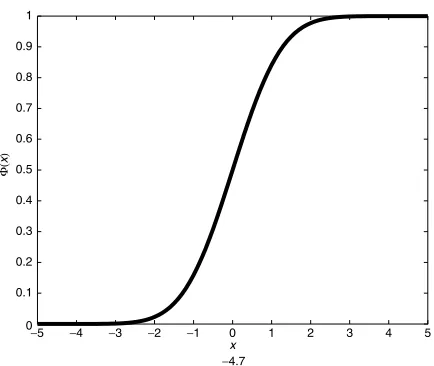
distribution (Figure 1.1). The cumulative distribution function
(z)=
z
−∞ 1
√
2πe −x2/2dx
is not obtainable in simple closed form, and requires either numerical ap-proximation or a table of values. The probability density functionf (x)is symmetric about 0 and appears roughly as follows.
The integral of the standard normal probability density function is 1, but to show this requires conversion to polar coordinates. If we square the integral of the normal probability density function, we obtain
∞
−∞ 1
√
2πe −1
2y2dy
∞
−∞ 1
√
2πe −1
2x2dx = 1 2π ∞ −∞ ∞ −∞e −1
2(x2+y2)dx dy
= 1 2π ∞ 0 2π 0
e−12r2rdθdr wherex =rcosθandy=rsinθ
=1
−5 −4 −3 −2 −1 0 1 2 3 4 5 0
0.05 0.1 0.15 0.2 0.25 0.3 0.35 0.4
x −4.8
φ(
x
[image:25.432.110.332.78.264.2])
FIGURE 1.1 The Standard Normal Probability Density Function
−5 −4 −3 −2 −1 0 1 2 3 4 5 0
0.1 0.2 0.3 0.4 0.5 0.6 0.7 0.8 0.9 1
Φ(
x
)
x −4.7
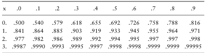
[image:25.432.113.330.349.532.2]T A B L E 1.1 Values of the Standard Normal Cumulative Distribution Function(x)
x .0 .1 .2 .3 .4 .5 .6 .7 .8 .9
0. .500 .540 .579 .618 .655 .692 .726 .758 .788 .816 1. .841 .864 .885 .903 .919 .933 .945 .955 .964 .971 2. .977 .982 .986 .989 .992 .994 .995 .997 .997 .998 3. .9987 .9990 .9993 .9995 .9997 .9998 .9998 .9999 .9999 .99995
We usually provide the values of the normal cumulative distribution function either through a function such asnormcdfin Matlab or through a table of values such as Table A1 (a much more compact version than that found at the back of most statistics books).
For example, we can obtain
(1.1)=0.864 (0.6)=0.726
(−0.5)=1−(0.5)=1−0.692
Note, for example that (−x) = 1−(x) for all x, and if Z has a standard normal distribution, we can find probabilities of intervals such as
P[−1< Z <1]≈0.68 and P[−2< Z <2]≈0.954
The General Normal Distribution If we introduce a shift in the location in the graph of the normal density as well as a change in scale, then the resulting random variable is of the form
X=µ+σZ Z∼N (01)
for some constants−∞<µ<∞σ>0. In this case, since
P (X≤x)=P
Z≤ x−µ
σ
=
x−µ
σ
it is easy to show by differentiating this with respect toxthat the probability density function ofXis
f (x;µσ)= √1
2πσe
−(x−µ)2/2σ2
[image:26.432.55.381.73.158.2]Moments Show that the functionf (x;µσ)integrates to 1 and is therefore a probability density function. It is not too hard to find the expected value and variance of a random variable having the probability density function
f (x;µσ)by integration:
E(X)=
∞
−∞
xf (x;µσ)dx=µ
var(X)=
∞
−∞(x−µ)
2f (x;µσ)dx=σ2
and this gives meaning to the parametersµ and σ2 the former being the
mean or expected value of the distribution and the latter the variance.
Linear Combinations of Normal Random Variables Suppose X1 ∼ N (µ1σ21) and
X2∼N (µ2σ22)are independent random variables. ThenX1+X2∼N (µ1+
µ2σ21+σ22). More generally if we sum independent random variables, each
having a normal distribution, the sum itself also has a normal distribution. The expected value of the sum is the sum of the expected values of the individual random variables, and the variance of the sum is the sum of the variances.
Problem Suppose Xi ∼N (µσ2)are independent random variables. What is the distribution of the sample mean
Xn= n
i=1Xi
n
Assumeσ=1and find the probabilityP[|Xn−µ|>0.1]for various values ofn. What happens to this probability asn→ ∞?
The Central Limit Theorem
The major reason that the normal distribution is the single most commonly used distribution is the fact that it tends to approximate the distribution of sums of random variables. For example, if we throwndice andSnis the sum of the outcomes, what is the distribution ofSn?The tables below provide the number of ways in which a given value can be obtained. The corresponding probability is obtained by dividing by 6n. For example, on the throw of
n=1die the probable outcomes are12 . . . 6with probabilities all1/6as indicated in Figure 1.3.
1 2 3 4 5 6 0
[image:28.432.145.299.58.180.2]0.02 0.04 0.06 0.08 0.1 0.12 0.14 0.16 0.18
FIGURE 1.3 The Sum ofn=1Discrete Uniform{1, 2, 3, 4, 5, 6}Random Variables
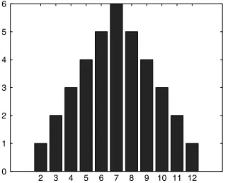
2 3 4 5 6 7 8 9 10 11 12 0
[image:28.432.140.301.220.349.2]1 2 3 4 5 6
FIGURE 1.4 The Sum ofn=2Discrete Uniform{1, 2, 3, 4, 5, 6}Random Variables
the values below:
Values 2 3 4 5 6 7 8 9 10 11 12
Probabilities×36 1 2 3 4 5 6 5 4 3 2 1
The probability histogram of these values is shown in Figure 1.4.
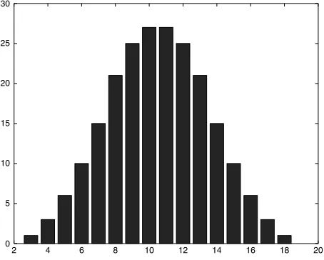
Finally, for the sum of the values on three independent dice, the values range from 3 to 18 and have probabilities which, when multiplied by 63,
result in the values
1 3 6 10 15 21 25 27 27 25 21 15 10 6 3 1
2 4 6 8 10 12 14 16 18 20 0
[image:29.432.106.333.59.241.2]5 10 15 20 25 30
FIGURE 1.5 The Distribution of the Sum of Three Discrete Uniform{1, 2, 3, 4, 5, 6} Random Variables
In general, these distributions show a simple pattern. For n = 1, the probability function is a constant (polynomial degree 0). Forn=2it is two linear functions spliced together. Forn=3, it is a spline consisting of three quadratic pieces (polynomials of degree n−1).In general, the histogram forSn, the sum of the values onnindependent dice, consists ofnpiecewise polynomials of degreen−1. These histograms rapidly approach the shape of the normal probability density function.
Example LetXi =0or1when theith toss of a biased coin is tails or heads, respectively. What is the distribution ofSn =
n
i=1Xi? Consider the
stan-dardized random variable obtained by subtractingE(Sn)and dividing by its standard deviation or the square root of var(Sn):
Sn∗= √Sn−np np(1−p)
Suppose we approximate the distribution ofSn∗ for large values ofn. First, consider a sequence of integers x =xnthat are close to the real numbernp+√np(1−p) in the sense that the difference is bounded by a constant. Mathematically we writex ∼np+z√np(1−p) for fixedzand 0< p <1.Then asn→ ∞,x/n→p. Stirling’s approximation tells us that
n!∼√2πnn+1/2eso that
n x
∼ √
2πnn+1/2e−n
2πxx+1/2(n−x)n−x+1/2∼
1
√
Also using the series expansion ln(1 +x) = x − 21x2 + Ox3, setting
σ=p(1−p)
n and noting thatσ→0asn→ ∞
ln p
x(1−p)n−x
(x n)x(1−
x n)n−x
=xln
p p+zσ
+(n−x)ln
1−p
1−p−zσ
= −xln
1+zσ
p
−(n−x)ln
1− zσ 1−p
= −n(p+zσ)ln
1+zσ
p
−n(1−p−zσ)ln
1− zσ 1−p
= −n(p+zσ)
zσ p −1 2 zσ p 2 +O zσ p 3
−n(1−p−zσ)
−
zσ
1−p
−1
2
zσ
1−p
2
+O
zσ
1−p
3
= −n zσ+z
2σ2
p −
1 2
z2σ2
p −zσ+
z2σ2
1−p −
1 2
z2σ2
1−p +O(σ
3)
= −1
2z
2σ2
n
p +
n
1−p
+O(n−1/2)= −z
2
2 +O(n −1/2)
Therefore,
P[Sn=x]=P[Sn∗=z]=
n x
px(1−p)n−x
∼ n x x n x
1−x
n
n−x px(1−p)n−x
(xn)x(1−x n)n−x
∼ √ 1
np(1−p)
1
√
2πe −z2/2
This is the standard normal probability density function multiplied by the distance between consecutive values ofSn∗. In other words, this result says that the area under the probability histogram forSn∗ for the bar around the point zcan be approximated by the area under the normal curve between the same two pointsz±2√ 1
np(1−p)
.
20 25 30 35 40 45 50 55 60 0
0.01 0.02 0.03 0.04 0.05 0.06 0.07 0.08 0.09
x
f(x)
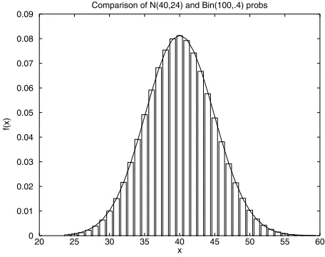
[image:31.432.105.333.58.238.2]Comparison of N(40,24) and Bin(100,.4) probs
FIGURE 1.6 Binomial(1000.4) Probability Histogram Together with N (4024)
Probability Density Function
distribution function of
Sn∗=
n
i=1√Xi−nµ
nσ
converges to the cumulative distribution function of a standard normal ran-dom variable.
Consider, for example, the case where the Xi are independent, each with a Bernoulli(p) distribution. Then the sum ni=1Xi has a binomial distribution with parameters n p and the above theorem asserts that if we subtract the mean and divide by the standard deviation of a binomial random variable, the result is approximately standard normal. In other words, for large values ofna binomial random variable is approximately normal(np np(1−p)). To verify this fact, we plot both the binomial(1000.4)
histogram as well as the normal probability density function in Figure 1.6.
Problem Use the central limit theorem and the normal approximation to a probability histogram to estimate the probability that the sum of the numbers on 5 dice is 15. Compare your answer with the exact probability.
normal distribution. The parameters are easily determined sinceE(aX+b)= aE(X)+bandvar(aX+b)=a2var(X).Is this true of arbitrary functions and
general distributions? For example, isX2normally distributed? The answer
in general isno. For example, the distribution ofX2 must be concentrated
entirely on the positive values of x whereas the normal distributions are all supported on the whole real line (i.e., the probability density function
f (x) >0allx∈R).In general, the safest method for finding the distribution of the function of a random variable in the continuous case is to first find the cumulative distribution of the function and then differentiate to obtain the probability density function. This allows us to verify the result below.
Theorem A9 Suppose a continuous random variableXhas probability density function fX(x).Then the probability density function of Y = h(X)where
h(.) is a continuous monotone increasing function with inverse function
h−1(y)is
fY(y)=fX(h−1(y))
d dyh
−1(y)
1.6
MOMENT-GENERATING FUNCTIONS
Consider a random variableX.We have seen several ways of describing its distribution, using either a cumulative distribution function, a probability density function (continuous case) or probability function, or a probabil-ity histogram or table (discrete case). We may also use some transform of the probability density or probability function. For example, consider the function
MX(t)=EetX
defined for all values oft such that this expectation exists and is finite. This function is called the moment-generating function of the (distribution of the) random variableX.It is a powerful tool for determining the distribution of sums of independent random variables and for proving the central limit theorem. In the discrete case we can writeMX(t)=
xextP[X=x], and in the continuous caseMX(t)=
∞
−∞extf (x)dx.The logarithm of the moment-generating functionln(MX(t))is called the cumulant-generating function.
Properties of the Moment-Generating Function For these properties we assume that the moment-generating function exists at least in some neighborhood of the valuet =0say for− < t < for some >0.We also assume that
d dtE[X
netX] = E[d dtX
netX] for each value ofn =012 . . .then for− <
under general conditions involving the rate at which the integral or series converges.
1. M(0)=E(X).
2. M(n)(0)=E(Xn) n=12 . . ..
3. A moment-generating function uniquely determines a distribution. In other words, if MX(t) = MY(t) for all − < t < then X and Y have the same distribution.
4. MaX+b(t)=ebtMX(at) for constantsa b.
5. IfXandY are independent random variables,MX+Y(t)=MX(t)MY(t).
Examples LetXhave a distribution as given in the first column of the table below. Then the moment-generating function ofXis as given in column 2.
Distribution Moment-Generating FunctionMX(t) Binomial(n p) (pet+1−p)n
Poisson(λ) exp{λ(et−1)} Exponential, meanµ 1
1−µt fort <1/µ Normal(µσ2) exp{µt+σ2t2/2}
Moment-generating functions are useful for showing that a sequence of cumulative distribution functions converge because of the following result. The result implies that convergence of the moment-generating functions can be used to show convergence of the cumulative distribution functions (i.e., convergence of the distributions).
Theorem A10 SupposeZnis a sequence of random variables with moment-generating functionsMn(t).LetZbe a random variableZhaving moment-generating function M(t). If Mn(t) → M(t)for all t in a neighborhood of0then
P[Zn≤z]→P[Z≤z]
asn→ ∞for all values ofzat which the functionFZ(z)is continuous.
1.7
JOINT DISTRIBUTIONS AND CONVERGENCE
do we construct a similar measure compatible with the notion of area in two-dimensional Euclidean space? We naturally begin with the measure of rect-angles or indeed anyproductset of the formA×B= {(x y);x ∈A y∈B}
for arbitrary (Borel) setsA⊂ B⊂ . The measure of a product set can be defined as the product of the measure of the two-factor setsµ(A×B)=λ(A)
λ(B). This defines a measure for any product set, and by an extension the-orem, since the product sets form a Boolean algebra, we can extend this measure to the sigma algebra generated by the product sets.
More formally, suppose we are given two measure spaces(MMµ)and
(N Nν). Define theproduct spaceto be the space consisting of pairs of objects, one from each ofM andN,
Ω=M×N = {(x y); x∈M y∈N}
The Cartesian product of two sets A ⊂ M B ⊂ N is denotedA×B = {(a b);a ∈A b∈B}. This is the analogue of a rectangle, a subset ofM×N, and it is easy to define a measure for such sets as follows. Define theproduct measure of product sets of the above form byπ(A×B)=µ(A)ν(B). The following theorem is a simple consequence of the Caratheodory extension theorem.
Theorem A11 The product measureπdefined on the product sets of the form
{A×B;A∈N B∈M}can be extended to a measure on the sigma algebra
σ{A×B;A∈NB∈M}of subsets ofM×N.
There are two cases of product measure of importance. Consider the sigma algebra on 2 generated by the product of the Borel sigma algebras
on. This is called the Borel sigma algebra in2. We can similarly define
the Borel sigma algebra onn.
Similarly, if we are given two probability spaces (Ω1F1 P1)and(Ω2F2
P2), we can construct aproduct measure Qon the Cartesian product space
Ω1×Ω2 such thatQ(A×B)=P1(A)P2(B) for allA ∈ F1 B ∈ F2.This
guarantees the existence of a product probability space in which events of the form A×Ω2 are independent of events of the form Ω1×B for A ∈
F1 B∈F2.
We say a sequence of random variables X1 X2 . . . is independentif
the family of sigma algebras σ(X1)σ(X2) . . .are independent; that is, for
Borel setsBn n=1 . . . N in, the events[Xn∈Bn] n=1 . . . Nform a mutually independent sequence of events so that
P[X1 ∈B1 X2∈B2. . . ,Xn∈Bn]=P[X1 ∈B1]P[X2∈B2]· · ·P[Xn∈Bn] The sequence is said to beidentically distributed if every random variable
We have already seen the following result, but we repeat it here, if only to get the flavor of the proof.
IfX Y are independent integrable random variables on the same prob-ability space, thenXY is also integrable and
E(XY )=E(X)E(Y )
Proof. Suppose first thatXandY are both simple functions,X=ciIAi Y = djIBj. Then X and Y are independent if and only if P (AiBj) = P (Ai)P (Bj) for alli j, and so
E(XY )=E[(ciIAi)(
djIBj)] = cidjE(IAiIBj) = cidjP (Ai)P (Bj)
=E(X)E(Y )
More generally, supposeX Yare nonnegative random variables and consider independent simple functionsXnincreasing toXandYnincreasing toY.Then
XnYnis a nondecreasing sequence with limitXY.Therefore, by the monotone convergence theorem,
E(XnYn)→E(XY ) On the other hand,
E(XnYn)=E(Xn)E(Yn)→E(X)E(Y ).
Therefore,E(XY )=E(X)E(Y ).The case of general (positive and negative
random variablesX Y we leave as a problem. I
Joint Distributions of More Than Two Random Variables SupposeX1 . . . Xn are random variables defined on the same probability space (ΩF P )(but not necessarily independent). The joint distribution can be characterized by the joint cumulative distribution function, a function onn defined by
F (x1 . . . xn)=P[X1≤x1 . . . Xn≤xn]=P ([X1≤x1]∩ · · · ∩[Xn≤xn]) The joint cumulative distribution function allows us to findP[a1< X1≤
b1 . . . an< Xn≤bn]. By the inclusion-exclusion principle,
P[a1< X1 ≤b1 . . . an< Xn≤bn]=F (b1 b2 . . . bn)
−
j
F (b1 . . . aj bj+1 . . . bn)
+
i<j
The formula (1.8) above allows us to construct the probability measure of any product of intervals
C=(a1 b1]×(a2 b2]× · · ·(an bn]
and thereby any disjoint union of finitely many sets of the formC.The class of all such disjoint unions (including all of n) forms an algebra of sets, closed under complements, finite unions and intersections. In the same way as we constructed Lebesgue measure on the Euclidean space n from the basic notion of the length of an interval, we can now extend this probability measure to all sets in the sigma algebra generated by setsCof the form above. In general, a joint cumulative distribution function defined onnallows us to define a probability measure onn−dimensional Euclidean space. However in order that a function qualify as a joint c.d.f., the following conditions need to be satisfied.
Theorem A12 The joint cumulative distribution function has the following properties:
(a) F (x1 . . . xn)is right-continuous and nondecreasing in each argument
xi when the other arguments xj j=i, are fixed.
(b) F (x1 . . . xn)→ 1asmin(x1 . . . xn)→ ∞and F (x1 . . . xn)→0as
min(x1 . . . xn)→ −∞.
(c) The expression on the right-hand side of(1.8) is greater than or equal to zero for all a1< b1 a2< b2 . . . an< bn.
The joint probability distribution of the variablesX1 . . . Xnis a mea-sure onRn.It can be determined from the cumulative distribution function in the usual fashion, first by defining the measure of intervals and then ex-tending this to the sigma algebra generated by these intervals. In order to verify that the random variables are mutually independent, it is sufficient to verify that the joint cumulative distribution function factors
F (x1 . . . xn)=F1(x1)F2(x2)· · ·Fn(xn)=P[X1≤x1]· · ·P[Xn≤xn] for allx1 . . . xn∈ .
Theorem A13 If the random variables X1 . . . Xnare mutually independent, then
E[
n
j=1
gj(Xj)]= n
j=1
E[gj(Xj)]
An infinite sequence of random variablesX1 X2 . . . is mutually
inde-pendent if every finite subset is mutually indeinde-pendent.
Definition: Strong (Almost Sure) Convergence Let X and Xn n = 12 . . . be random variables all defined on the same probability space(ΩF). We say that the sequence Xn convergesalmost surely(orwith probability1) toX (denoted Xn→X a.s.) if the event
{ω;Xn(ω)→X(ω)} = ∩∞m=1
|Xn−X| ≤
1
m a.b.f.o.
has probability 1. Here the notationa.b.f.o., standing for “all but finitely often,” is the “liminf” of the events[|Xn−X| ≤ m1].
In order to show that a sequenceXnconverges almost surely, we need thatXnare (measurable) random variables for alln, and to show that there is some measurable random variableXfor which the set{ω;Xn(ω)→X(ω)} is measurable and hence an event, and that the probability of this event
P[Xn → X]is 1. Alternatively, we can show that for each value of >0
P[|Xn−X|> i.o.]=0or in other words, that the probability of the set of all pointsωsuch thatXn(ω)does not converge toX(ω)is zero. It is sufficient to consider values of of the form =1/m,m=12 . . .above.
The law of large numbers (sometimes called the law of averages) is the best-known result in probability. It says, for example, that the average of independent Bernoulli random variables, or Poisson, or negative binomial, or gamma random variables, to name a few, converge to their expected value with probability 1.
Theorem A14 (Strong Law of Large Numbers) IfXn n=12 . . . is a sequence of independent identically distributed random variables withE|Xn|<∞(i.e., they are integrable) andE(Xn)=µ, then
1
n
n
i=1
Xi→µalmost surely asn→ ∞
1.8
WEAK CONVERGENCE (CONVERGENCE IN DISTRIBUTION)
Consider random variables that are constants:Xn(w)=1+1nfor allw. By any sensible definition of convergence,Xnconverges toX =1asn → ∞. Does the cumulative distribution function ofXn sayFn converge to the cumulative distribution function ofXpointwise? In this case it is true that
Fn(x)→F (x)at all values ofxexcept the valuex =1, where the function
convergence in law) is defined as pointwise convergence of the c.d.f. at all values ofx except those at whichF (x)is discontinuous. Of course, if the limiting distribution is absolutely continuous (for example, the normal dis-tribution as in the Central Limit Theorem), thenFn(x) → F (x)does hold for all values ofx.
Definition: Weak Convergence If Fn(x) n=1 . . ., is a sequence of cumulative distribution functions and if F is a cumulative distribution function, we say that Fn converges to F weaklyorin distributionif Fn(x) → F (x) for all x at which F (x) is continuous. Weak convergence of a sequence of random variables Xn whose c.d.f. converges in the above sense is denoted in a variety of ways, such asXn⇒XorXn →DX(hereD stands for “in distribution”).
There are simple examples of cumulative distribution functions that con-verge pointwise but not to a genuine cumulative distribution because some of the mass of the distribution escapes to infinity. For example, ifFnis the cu-mulative distribution function of a point mass at the pointn, thenFn(x)→0 for each fixed value ofx <∞.An additional condition, called tightness, is needed to ensure that the limiting distribution is a “proper” probability dis-tribution (i.e., has total measure 1). A sequence of probability measuresPn on Euclidean space istightif for all >0there exists a bounded rectangle
K such thatPn(K) >1− for alln.A sequence of cumulative distribution functionsFndefined onRis tight if, for every >0there is a real number
M < ∞ such that the probabilities of interval [−M M] are greater than than1−
Fn(M)−Fn(−M)≤1− for alln=12 ...
Tightness is a condition that ensures that none of the probability mass es-capes to infinity. For example suppose a sequence of cumulative distribution functionsFn(x)converges to some limiting right-continuous functionF (x) at all continuity pointsxofF and suppose the sequenceFnis tight. Then it is easy to show that the limiting functionF is a proper cumulative distribution function (i.e. has total mass1)and the convergence is in distribution.
There is an alternative definition of weak convergence that is more ap-propriate for more general spaces of random elements such as spaces of continuous time stochastic processes.
General Definition of Weak Convergence A sequence of random elements of a metric space Xn converges weakly to X (i.e., Xn ⇒ X) if and only if
Definition: Convergence in Probability We say a sequence of random variables
Xn→Xin probabilityif for all >0,P[|Xn−X|> ]→0as n→ ∞. Convergence in probability is in general a somewhat more demanding concept than weak convergence, but less demanding than almost sure con-vergence. In other words, convergence almost surely implies convergence in probability, and convergence in probability implies weak convergence.
Theorem A15 If Xn→X almost surely,then Xn→X in probability. However, convergence in probability does not imply convergence almost surely,but it does imply weak convergence.
Theorem A16 IfXn→Xin probability,thenXn→DX.
The converse of this theorem holds under one condition, when the con-vergence in distribution s to a constant.
Theorem A17 If Xn →Dconverges in distributionto some constantc, then
Xn→cin probability.
The next result, Fubini’s theorem, allows us to change the order of inte-gration as long as the function being integrated is, in fact, integrable.
Theorem A18 (Fubini’s Theorem) Suppose g(x y)is integrable with respect to a product measure π=µ×νon M×N. Then
M×N
g(x y)dπ=
M
N
g(x y)dν
dµ=
N
M
g(x y)dµ
dν
Convolutions Consider two independent random variablesX Y, both having a discrete distribution. Suppose we wish to find the probability function of the sumZ=X+Y. Then
P[Z=z]=
x
P[X=x]P[Y =z−x]=
x
fX(x)fY(z−x)
Similarly, ifX Y are independent, absolutely continuous distributions with probability density functions fX fY, respectively, then we find the proba-bility density function of the sumZ=X+Y by
fZ(z)= ∞
In both the discrete and continuous cases, we can rewrite the above in terms of the cumulative distribution function FZ of Z. In either case,
FZ(z)=E[FY(z−X)]=
FY(z−x)FX(dx)
We use the last form as a more general definition of aconvolutionbetween two cumulative distribution functions F G. We define theconvolutionof
F and G to be F ∗G(x) = −∞∞ F (x−y)dG(y).
Properties of Convolution
(a) IfF Gare cumulative distributions functions, then so is F ∗G. (b) F ∗G=G∗F.
(c) If eitherF orGis absolutely continuous with respect to Lebesgue mea-sure, then F ∗G is absolutely continuous with respect to Lebesgue measure.
The convolution of two cumulative distribution functionsF ∗G repre-sents the c.d.f of the sum of two independent random variables, one with c.d.f.F and the other with c.d.f.G.
1.9
STOCHASTIC PROCESSES
A stochastic process is an indexed family of random variablesXt fort rang-ing over some index setT, such as the integers or an interval of the real line. For example, a sequence of independent random variables is a stochastic process, as is a Markov chain. For an example of a continuous-time stochas-tic process, defineXt to be the price of a stock at timet (assuming trading occurs continuously over time).
Markov Chains Consider a sequence of (discrete) random variablesX1 X2 . . .
each of which takes integer values12 . . . N(calledstates). We assume that for a certain matrixP (called thetransition probability matrix), the condi-tional probabilities are given by corresponding elements of the matrix,
P[Xn+1=j|Xn=i]=Pij i =1 . . . N j =1 . . . N
and furthermore that the chain cares only about the last state occupied in determining its future:
PXn+1=j|Xn=i Xn−1=i1 Xn−2=i2· · ·Xn−l =il
for allj i i1 i2 . . . ilandl =23 . . .. Then the sequence of random vari-ablesXnis called aMarkov chain. Markov chain models are the most com-mon simple models for dependent variables, including weather (precipita-tion, temperature), movements of security prices, and others. They allow the future of the process to depend on the present state of the process