Numerical Methods
26
0
0
Full text
(2) Lecture Notes for Numerical Methods, FEQA MSc. THE BUSINESS SCHOOL FOR FINANCIAL MARKETS. What Influences Implied Volatility?. • Implied volatility σ depends on: – the price of the underlying S – the market price of the option C – the strike of the option K – the maturity of the option t – the interest rate r – and any other variables that influence the price of the option.. 3. Prof. C.O. Alexander. THE BUSINESS SCHOOL FOR FINANCIAL MARKETS. Black-Scholes Formula. If prices are governed by geometric Brownian motion (GBM) and there is perfect replication, then the current price of a call option C has a closed form analytic solution: C = SN(x) - Ke-rtN(x-σ σ√t) where x measures the ‘moneyness’ of the option: x = ln(S/Ke-rt) / σ√t + σ√t / 2. In-the-money (ITM) x>0 At-the-money (ATM) x=0 Out-of-the-money (OTM) x<0. and N(x) is the normal distribution function Prof. C.O. Alexander. Copyright ISMA centre, January 2000. 4.
(3) Lecture Notes for Numerical Methods, FEQA MSc. THE BUSINESS SCHOOL FOR FINANCIAL MARKETS. Black-Scholes Implied Volatilities. • The values of S, K, r and t are all observable, so the volatility which is ‘implied’ in an observed market price C can be computed. • No analytic form exists, but numerical methods (described in Chriss pp330-340) are used to approximate the value of the implicit function σ = f( C, S, K, r, t). • Usually volatility is quoted as an annualized percentage: Volatility = 100 σ √250 % 5. Prof. C.O. Alexander. Example. THE BUSINESS SCHOOL FOR FINANCIAL MARKETS. From the FT on June 15th ‘99: FTSE 100 Index options expiring on 18th June ‘99. Strike 6250 6300 6350 6400 6450 6500 6550 6600 6650 6700. Price 223 176 132 92 58.5 33 16 5.5 2 0.5. Calls vol 29.21 26.32 24.26 22.51 21.42 19.53 19.23 18.59. Volume 10 1 2 18 30 178 400 1966 0 1. Price 4 6.5 12.5 23 40 66.5 102.5 149 199 249. Puts vol 23.65 21.55 20.4 19.28 17.9 16.57 14.48 14.05 -. The closing price on the FTSE was 6451.2. Prof. C.O. Alexander. Copyright ISMA centre, January 2000. Volume 120 37 2 22 64 12 0 3 0 0. 6.
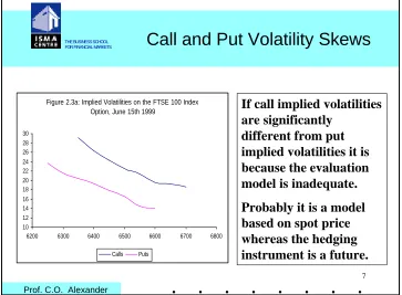
(4) Lecture Notes for Numerical Methods, FEQA MSc. Call and Put Volatility Skews. THE BUSINESS SCHOOL FOR FINANCIAL MARKETS. If call implied volatilities are significantly different from put implied volatilities it is because the evaluation model is inadequate.. Figure 2.3a: Implied Volatilities on the FTSE 100 Index Option, June 15th 1999 30 28 26 24 22 20 18 16 14 12 10 6200. 6300. 6400. 6500 Calls. 6600 Puts. 6700. 6800. Probably it is a model based on spot price whereas the hedging instrument is a future. 7. Prof. C.O. Alexander. THE BUSINESS SCHOOL FOR FINANCIAL MARKETS. Why the Differences between Call and Put Implied Volatilities ?. • On June 15th 1999 the FTSE 100 future closed at 6486, but its theoretical fair value was 6453.92 • So the market price of a call was based on 6486 but the model price of the a call was based on 6453.92 • Market prices of call options therefore appear to be very expensive and the only way that the model can account for the high market price is to jack up the volatility. • Similarly puts will appear less expensive than they should, so the implied volatility that is backed out of the model will be lower. 8. Prof. C.O. Alexander. Copyright ISMA centre, January 2000.
(5) Lecture Notes for Numerical Methods, FEQA MSc. THE BUSINESS SCHOOL FOR FINANCIAL MARKETS. Differences between Implied and Statistical Volatility. • Implied volatilities and statistical volatilities are both forecasting the same thing: the volatility of the underlying asset over the life of the option. • But the two types of volatility measure often differ. • Because they use different data and different models:. 30-day Volatility Forecasts GBP-USD 25 20 15 10 5 0 May-88 May-89 May-90 May-91 May-92 May-93 May-94 May-95 GARCH30. EWMA. HIST30. IMP30. 9. Prof. C.O. Alexander. THE BUSINESS SCHOOL FOR FINANCIAL MARKETS. Differences between Implied and Statistical Volatility. Implied volatility. Statistical volatility. Model is based on GBM:. Return distributions are:. dS/S = µ dt + σ dz – price increments are governed by a Wiener process (so they are independent and normal) – the volatility σ of the underlying asset S is constant.. • Unconditional – constant volatility – weighted averages. • Conditional – stochastic volatility – GARCH or Diffusion. 10. Prof. C.O. Alexander. Copyright ISMA centre, January 2000.
(6) Lecture Notes for Numerical Methods, FEQA MSc. THE BUSINESS SCHOOL FOR FINANCIAL MARKETS. Differences between Implied and Statistical Volatility. If statistical volatilities were correct, then differences between the implied and statistical measures of volatility would reflect a mis-pricing of the option. That is, the wrong option model is being used, or investors have irrational expectations. If implied volatilities were correct (so the option pricing model is an accurate representation of reality, and investors expectations are correct so that there is no over- or under- pricing in the options market), then any observed differences between implied and statistical volatilities would reflect inaccuracies in the statistical forecast. 11. Prof. C.O. Alexander. THE BUSINESS SCHOOL FOR FINANCIAL MARKETS. 2. Smiles, Skews and Volatility Term Structures. • The smile effect in implied volatility refers to the fact that OTM options have higher implied volatilities than ATM options. • Thus the plot of implied volatility vs moneyness (or strike) on a given day, for all options of a fixed maturity, will be ‘smile’ shaped Implied Volatility, σ. • The smile effect tends to increase as the option approaches expiry. 0 Prof. C.O. Alexander. Copyright ISMA centre, January 2000. Moneyness, x 12.
(7) Lecture Notes for Numerical Methods, FEQA MSc. THE BUSINESS SCHOOL FOR FINANCIAL MARKETS. Reasons for the Smile. • The volatility smile is a result of pricing model bias, and would not be found if options were priced using an appropriate model. • Black-Scholes is based on the assumption of GBM. But Volatility is not constant, and neither are returns normally distributed. • Thus OTM options have a greater chance of ending up ITM than the Black-Scholes formula allows. • Consequently the Black-Scholes formula is biased to underprice OTM options. • This under-pricing of the model compared to observed market behaviour yields higher implied volatilities for OTM options. 13. Prof. C.O. Alexander. THE BUSINESS SCHOOL FOR FINANCIAL MARKETS. Reasons for the Skew. • The problem is compounded in equity markets because they often exhibit a leverage effect. • That is volatility is often higher following market falls than it is following market rises of the same magnitude. • So OTM puts require higher volatility to end up in-themoney than do OTM calls. • This induces a pronounced negative ‘skew’ in the volatility smile.. 14. Prof. C.O. Alexander. Copyright ISMA centre, January 2000.
(8) Lecture Notes for Numerical Methods, FEQA MSc. Volatility Term Structures. THE BUSINESS SCHOOL FOR FINANCIAL MARKETS. • On any fixed date a plot of the fixed-strike implied volatilities of different maturities gives a term structure of volatilities • For example for the 6425 strike the implied volatility term structure on 15th June 1999 looked something like this: 25%. 20%. months 15. Prof. C.O. Alexander. THE BUSINESS SCHOOL FOR FINANCIAL MARKETS. Expiry end: Strike 6275 6325 6375 6425 6475 6525 6575 6625. Call. Financial Times Prices of the FTSE 100 Index European Options on June 15th 1999. Jun Put. 169 126.5 89 57 33 16 6.5 2. 11 19 31 49 75 108 148.5 194. Call 281 245 214 184 154.5 128.5 104 83. Jul Put 101 115 133.5 154 174 197.5 223 252. Aug Call Put 366.5 332.5 300 269.5 240 213 187 163.5. 182 197.5 215 233.5 254 276 300 326. Sep Put. Call. 397. 244. 582.5. 373. 333. 279. 517.5. 405.5. 272. 316.5 272. 448. 219. 362. 495.5. Call. 219. Dec Put. 16. Prof. C.O. Alexander. Copyright ISMA centre, January 2000.
(9) Lecture Notes for Numerical Methods, FEQA MSc. THE BUSINESS SCHOOL FOR FINANCIAL MARKETS. Behaviour of Volatility Term Structures. • Long term volatilities will change much less than short term volatilities • Volatility term structures mean revert to the long term average • They may slope upwards or downwards, although they are not generally monotonic. Current Market Conditions. Slope of Term Structure. Volatile. Downwards. Tranquil. Upwards 17. Prof. C.O. Alexander. THE BUSINESS SCHOOL FOR FINANCIAL MARKETS. • A smile surface is a surface plot of implied volatilities for different strikes (or moneyness) and maturities • Slicing through this surface at a fixed strike or moneyness gives a volatility term structure • Slicing through this surface at a fixed maturity gives a smile, which becomes more pronounced as maturity decreases. The Smile Surface Figure 13: Smile surface of the FTSE, De 1. Implied Volatlity 1 0.8 0.6 0.4 0.2 0 -0.6. 400 -0.4. -0.2 Moneyness. 0. Prof. C.O. Alexander. Copyright ISMA centre, January 2000. 200 0.2 0. Maturity 18.
(10) Lecture Notes for Numerical Methods, FEQA MSc. THE BUSINESS SCHOOL FOR FINANCIAL MARKETS. Fitting Smile Surfaces. • Reliable market data for all strikes and maturities are not available • Data on OTM or very long term options is particularly unreliable since quotes may be left unchanged for days when trading is thin • So smile surfaces must be interpolated using numerical methods such as cubic splines (see Numerical recipes in C).. 19. Prof. C.O. Alexander. THE BUSINESS SCHOOL FOR FINANCIAL MARKETS. Use of Smile Surfaces in Dynamic Delta Hedging. • The most basic dynamic hedge is to match a position in the underlying with an amount N(x) of an option • This is hedge ratio is the option delta, and since x = ln(S/Ke-rt) / σ√t + σ√t / 2 its value depends very much on implied volatility and maturity, as predicted by the current smile surface • As the underlying moves over time, the position will need constant re-balancing to be delta neutral • So, over a period of time, very large losses might be made if the wrong hedging volatility is used 20. Prof. C.O. Alexander. Copyright ISMA centre, January 2000.
(11) Lecture Notes for Numerical Methods, FEQA MSc. 3. Volatility Regimes. THE BUSINESS SCHOOL FOR FINANCIAL MARKETS. 6750. 70.00. 6500. 60.00. 6250 50.00. 6000 40.00. 5750. 30.00. 5500 5250. 20.00. 5000 10.00. Mar-99. Feb-99. Jan-99. Dec-98. Nov-98. Oct-98. Sep-98. Aug-98. Jul-98. Jun-98. Apr-98. May-98. Mar-98. Feb-98. 4750 Jan-98. 0.00. 4500. 4025. 4075. 4125. 4175. 4225. 4275. 4325. 4375. 4425. 4475. 4525. 4575. 4625. 4675. 4725. 4775. 4825. 4875. 4925. 4975. 5025. 5075. 5125. 5175. 5225. 5275. 5325. 5375. 5425. 5475. 5525. 5575. 5625. 5675. 5725. 5775. 5825. 5875. 5925. 5975. 6025. 6075. 6125. 6175. 6225. 6275. 6325. 6375. 6425. 6475. 6525. 6575. 6625. 6675. 6725. 6775. 6825. 6875. 6925. 6975. ATM. FTSE100. How should we model movements in implied volatility smile surfaces as the underlying price moves?. 21. Prof. C.O. Alexander. THE BUSINESS SCHOOL FOR FINANCIAL MARKETS. Derman’s ‘Sticky’ Models. 1. Sticky Strike. 2. Sticky Delta. 3. Sticky Tree. Bounded Market. Trending Market. Jumpy Market. σK = σ0 - b(K-S0). σK = σ0 - b(K-S). σK = σ0 - b(K+S). σK independent of S. σK increases with S. σK decreases with S. σATM = σ0 - b(S-S0). σATM = σ0. σATM = σ0 - 2bS. σATM decreases as price increases. σATM independent of price. σATM moves twice as fast as the skew 22. Prof. C.O. Alexander. Copyright ISMA centre, January 2000.
(12) Lecture Notes for Numerical Methods, FEQA MSc. Modelling the Relationship between ATM Volatility and Price. THE BUSINESS SCHOOL FOR FINANCIAL MARKETS. 0.006 Probability. 0.005 0.004. First question: How is ATM implied volatility likely to move as the underlying price changes?. 0.003 0.002 0.001 0 Change in Equity Index. Change in ATM Implied Volatility. 23. Prof. C.O. Alexander. Scatter Plots. THE BUSINESS SCHOOL FOR FINANCIAL MARKETS. Daily changes in FTSE and 1mth ATM vol. Daily changes in FTSE and 3mth ATM vol. 10. 10. 8. 8. 6. 6. 4. 4. 2. 2. 0 -250. -200. -150. -100. -50. -2. 0 0. 50. 100. 150. 200. 250. -250. -200. -150. -100. -50. -2. -4. -4. -6. -6. -8. -8. -10. -10. 0. 50. 100. 150. 200. 24. Prof. C.O. Alexander. Copyright ISMA centre, January 2000. 250.
(13) Lecture Notes for Numerical Methods, FEQA MSc. Scatter Plots. THE BUSINESS SCHOOL FOR FINANCIAL MARKETS. Daily Change in Cable and 1M Imp Vol. Daily Change in Cable and 3M Imp Vol 3. 8. 2.5. 6. 2 1.5. 4. 1 0.5. 2 -0.08. 0 -0.08. -0.06. -0.04. -0.02. 0. 0.02. 0.04. -0.06. -0.04. 0 -0.02 -0.5 0. 0.02. 0.04. -1. 0.06. -2. -1.5. -4. -2.5. -2. 25. Prof. C.O. Alexander. THE BUSINESS SCHOOL FOR FINANCIAL MARKETS. Constructing a Joint Distribution of ∆S and ∆σATM. 0.007 Probability. 0.006 0.005 0.004 0.003 0.002 0.001 0. Change in Implied Volatility. Change in Index. prob(∆σATM and ∆S) = prob(∆σATM∆S) prob(∆S) 26. Prof. C.O. Alexander. Copyright ISMA centre, January 2000. 0.06.
(14) Lecture Notes for Numerical Methods, FEQA MSc. Estimating prob(∆σATM∆S). THE BUSINESS SCHOOL FOR FINANCIAL MARKETS. • To give conditional probabilities prob(∆σATM∆S) one needs to model the relationship between implied volatility and the price. • The linear model of ATM implied volatility and the price has been employed: ∆σATM = α + β ∆S + ε in which case ∆σATM | ∆S ∼ N(α + β ∆S , σε2). 27. Prof. C.O. Alexander. Daily Data on σATM and S. THE BUSINESS SCHOOL FOR FINANCIAL MARKETS. 60. 6500. 55. 6250. 50 6000 45 5750 40 35. 5500. 30. 5250. 25 5000 20 4750. ATM. Mar-99. Mar-99. Jan-99. Feb-99. Jan-99. Feb-99. Dec-98. Dec-98. Nov-98. Oct-98. Oct-98. Nov-98. Oct-98. Sep-98. Sep-98. Aug-98. Jul-98. Jul-98. Aug-98. Jun-98. Jun-98. May-98. Apr-98. May-98. Apr-98. Mar-98. Mar-98. Jan-98. Feb-98. Feb-98. Jan-98. 10. Jan-98. 15. 4500. Does the FTSE100 index price have a negative relationship with 3 month ATM volatility?. FTSE100. 28. Prof. C.O. Alexander. Copyright ISMA centre, January 2000.
(15) Lecture Notes for Numerical Methods, FEQA MSc. Daily Data on σATM and S. THE BUSINESS SCHOOL FOR FINANCIAL MARKETS. 25. 2.20. 20. Does the Cable rate have a negative relationship with 1 month ATM volatility?. 2.00. 15 1.80 10 1.60. 5. 1M Imp Vol. Jul-95. Jul-94. Jan-95. Jul-93. Jan-94. Jan-93. Jul-92. Jul-91. Jan-92. Jan-91. Jul-90. Jul-89. Jan-90. Jan-89. Jul-88. 1.40 Jan-88. 0. Daily Clo. 29. Prof. C.O. Alexander. ∆σATM = α + β ∆FTSE + ε. THE BUSINESS SCHOOL FOR FINANCIAL MARKETS. Coefficient on Daily Change in FTSE. Significance of Coefficient on Daily Change in FTSE. 0. 0. -0.005. -2 -4. -0.01. -6. -0.015. -8 -0.02. -10. -0.025. Beta (1mth ATM). Beta (2mth ATM). Beta (3mth ATM). tstat (1mthATM). Jan-99. tstat (3mthATM). 30. Prof. C.O. Alexander. Copyright ISMA centre, January 2000. Feb-99 Mar-99. Dec-98. Oct-98. tstat (2mthATM). Nov-98. Aug-98. Sep-98. Jun-98 Jul-98. Apr-98. May-98. Jan-98. Jan-99. Feb-99 Mar-99. Nov-98 Dec-98. Oct-98. Aug-98. Sep-98. Jun-98 Jul-98. -16 Apr-98 May-98. -0.035 Jan-98 Feb-98 Mar-98. -14. Feb-98 Mar-98. -12. -0.03.
(16) Lecture Notes for Numerical Methods, FEQA MSc. THE BUSINESS SCHOOL FOR FINANCIAL MARKETS. Prob(∆S). • We shall assume that prob(∆S) is represented by a normal density ∆S ∼ N(µ, σ2) • The parameters could be obtained from statistical forecasts of the mean and variance. • Their values will depend very much on current market circumstances.. 31. Prof. C.O. Alexander. THE BUSINESS SCHOOL FOR FINANCIAL MARKETS. …on 31st March ‘99. • Assume the index was fairly stable, as reflected by a marginal density for one-day changes in FTSE100 of ∆S ∼ N(0, 352). • The OLS estimate of a linear relationship between the one-day changes in 1 month ATM volatility ∆σATM and ∆S on 31.03.99 was: ∆σATM = -0.3 - 0.017 ∆S (-2.73) (-10.01). s.e. regression = 0.492. ⇒ ∆σATM | ∆S ∼ N(−0.3 − 0.017 ∆S , 0.4922) 32. Prof. C.O. Alexander. Copyright ISMA centre, January 2000.
(17) Lecture Notes for Numerical Methods, FEQA MSc. THE BUSINESS SCHOOL FOR FINANCIAL MARKETS. Prob(∆σATM and ∆S) in a Stable Market FTSE100 31 Mar 99. 0.01 Probability. 0.009 0.008 0.007 0.006 0.005 0.004 0.003 0.002 0.001 0. Change in Implied Volatility. Change in Index. ∆S ∼ N(0, 352), ∆σATM | ∆S ∼ N(−0.3−0.017 ∆S , 0.4922) 33. Prof. C.O. Alexander. THE BUSINESS SCHOOL FOR FINANCIAL MARKETS. Prob(∆σATM and ∆S) in a Jumpy Market FTSE100 9th Oct 98. 0.01 Probability. 0.009 0.008 0.007 0.006 0.005 0.004 0.003 0.002 0.001 0. Change in Implied Volatility. ∆S ∼ N(−30, 602),. Change in Index. ∆σATM | ∆S ∼ N(-0.03 ∆S, 1.252) 34. Prof. C.O. Alexander. Copyright ISMA centre, January 2000.
(18) Lecture Notes for Numerical Methods, FEQA MSc. 4. Principal Component Models of the Smile. THE BUSINESS SCHOOL FOR FINANCIAL MARKETS. FTSE100 Index, 3 month ATM Volatility and the Skew: Jan ‘98 to Mar ‘99 60.00. 6500. 55.00. 6250. 50.00 6000 45.00 40.00. 5750. 35.00. 5500. 30.00. 5250. 25.00 5000 20.00 4750 Mar-99. Feb-99. Jan-99. Dec-98. Nov-98. Oct-98. Sep-98. Aug-98. Jul-98. Jun-98. May-98. Apr-98. Mar-98. Feb-98. 10.00. Jan-98. 15.00. 4500. 4025. 4125. 4225. 4325. 4425. 4525. 4625. 4725. 4825. 4925. 5025. 5125. 5225. 5325. 5425. 5525. 5625. 5725. 5825. 5925. 6025. 6125. 6225. 6325. 6425. 6525. 6625. 6725. 6825. 6925. ATM. FTSE100. 35. Prof. C.O. Alexander. Relationship between the Index and the Skew Deviations. THE BUSINESS SCHOOL FOR FINANCIAL MARKETS. Deviation of fixed strike volatility from ATM volatility 3 months 25.00. 6500. 20.00. 6250. 15.00 6000 10.00 5.00. 5750. 0.00. 5500. -5.00. 5250. -10.00 5000 -15.00 4750 Mar-99. Feb-99. Jan-99. Dec-98. Nov-98. Oct-98. Sep-98. Aug-98. Jul-98. Jun-98. May-98. Apr-98. Mar-98. Feb-98. -25.00. Jan-98. -20.00. 4500. 4025. 4125. 4225. 4325. 4425. 4525. 4625. 4725. 4825. 4925. 5025. 5125. 5225. 5325. 5425. 5525. 5625. 5725. 5825. 5925. 6025. 6125. 6225. 6325. 6425. 6525. 6625. 6725. 6825. 6925. FTSE100. 36. Prof. C.O. Alexander. Copyright ISMA centre, January 2000.
(19) Lecture Notes for Numerical Methods, FEQA MSc. Relationship between the Index and the Skew Deviations. THE BUSINESS SCHOOL FOR FINANCIAL MARKETS. 1 month 40. 6500. 35 6250. 30 25. 6000. 20 5750. 15 10. 5500. 5 0. 5250. -5 5000. -10 -15. 4750. 4500. Mar-99. Feb-99. Jan-99. Dec-98. Nov-98. Oct-98. Sep-98. Aug-98. Jul-98. Jun-98. May-98. Apr-98. Mar-98. Feb-98. -25. Jan-98. -20. 4025. 4075. 4125. 4175. 4225. 4275. 4325. 4375. 4425. 4475. 4525. 4575. 4625. 4675. 4725. 4775. 4825. 4875. 4925. 4975. 5025. 5075. 5125. 5175. 5225. 5275. 5325. 5375. 5425. 5475. 5525. 5575. 5625. 5675. 5725. 5775. 5825. 5875. 5925. 6025. 6075. 6125. 6175. 6225. 6275. 6325. 6375. 6725. 37 6775. 6425. 6475. 6525. 6575. 6625. 6825. 6875. 6925. 6975. FTSE100. Prof. C.O. Alexander. THE BUSINESS SCHOOL FOR FINANCIAL MARKETS. 6675. 5975. Why Does σK - σATM Increase with S? σK - σATM = -b (K - S). 1. Sticky Strike. 2. Sticky Delta. 3. Sticky Tree. Bounded Market. Trending Market. Jumpy Market. σK = σ0 - b(K-S0). σK = σ0 - b(K-S). σK = σ0 - b(K+S). σK independent of S. σK increases with S. σK decreases with S. σATM = σ0 - b(S-S0). σATM = σ0. σATM = σ0 - 2bS. σATM decreases as index increases. σATM independent of index. σATM moves twice as fast as the skew. 38. Prof. C.O. Alexander. Copyright ISMA centre, January 2000.
(20) Lecture Notes for Numerical Methods, FEQA MSc. THE BUSINESS SCHOOL FOR FINANCIAL MARKETS. How Should the Skew be Modified as the Index Changes?. • Step 1: Model the skew deviations from ATM volatility with a principal component analysis on ∆(σK(t) - σATM(t)). • Step 2: Model the relationship between the Index and the skew deviations as: ith principal component (t) = γ0,i (t) + γi (t) ∆FTSE + ηi (t) [t = option maturity (1mth, 2mth or 3mth)]. 39. Prof. C.O. Alexander. THE BUSINESS SCHOOL FOR FINANCIAL MARKETS. PCA of the Skew Deviations. • A principal components analysis of the daily change in σK - σATM shows that typically 80-90% of the variation in σK - σATM can be explained by 3 principal components. • The factor weights show that the principal components are capturing: – parallel shift (PC1) – tilt (PC2) – convexity (PC3). 40. Prof. C.O. Alexander. Copyright ISMA centre, January 2000.
(21) Lecture Notes for Numerical Methods, FEQA MSc. THE BUSINESS SCHOOL FOR FINANCIAL MARKETS. Variation Explained by Principal Components. 3 month data. Eigenvalue. Cumulative R2. PC1 PC2 PC3. 13.3574 2.257596 0.691317. 0.742078 0.8675 0.905906. 2 month data. Eigenvalue. Cumulative R2. PC1 PC2 PC3. 19.68491 0.866442 0.834766. 0.855866 0.893537 0.929831. 1 month data. Eigenvalue. Cumulative R2. PC1 PC2 PC3. 25.7177 11.6942 6.119627. 0.476254 0.692813 0.806139 41. Prof. C.O. Alexander. THE BUSINESS SCHOOL FOR FINANCIAL MARKETS. Strike 4225 4325 4425 4525 4625 4725 4825 4925 5025 5125 5225 5325 5425 5525 5625 5725 5825 5925. Factor Weights in PCA of σK - σATM PC1 0.53906 0.6436 0.67858 0.8194 0.84751 0.86724 0.86634 0.80957 0.9408 0.92639 0.92764 0.93927 0.93046 0.90232 0.94478 0.94202 0.93583 0.90699. PC2 0.74624 0.7037 0.58105 0.48822 0.34675 0.1287 0.017412 -0.01649 -0.18548 -0.22766 -0.21065 -0.22396 -0.25167 -0.20613 -0.2214 -0.22928 -0.22818 -0.22788. PC3 0.26712 0.1862 0.035155 -0.03331 -0.19671 -0.41161 -0.43254 -0.28777 0.068028 0.13049 0.12154 0.14343 0.16246 0.017523 0.073863 0.073997 0.074602 0.068758. 3 months. 42. Prof. C.O. Alexander. Copyright ISMA centre, January 2000.
(22) Lecture Notes for Numerical Methods, FEQA MSc. ith PC = γ0,i + γi ∆FTSE + ηi. THE BUSINESS SCHOOL FOR FINANCIAL MARKETS. 30. γ1 (parallel shift) is always positive and usually very highly significant.. 25 20 15 10 5 0 -5 -10. tstat on pc1. tstat on pc2. Mar-99. Jan-99. Feb-99. Nov-98. Dec-98. Oct-98. Sep-98. Jul-98. Aug-98. Jun-98. Apr-98. May-98. γ3 (convexity) often has the opposite sign to γ2.. Mar-98. Jan-98. -15 Feb-98. γ2 (tilt) is often negative (stable market) but sometimes positive (jumpy market) or zero (trending market).. tstat on pc3. 43. Prof. C.O. Alexander. What Happens to σK - σATM as the Index Increases in a Stable Market?. THE BUSINESS SCHOOL FOR FINANCIAL MARKETS. σK - σATM. σK - σATM γ1 > 0. γ2 < 0. + K (a) σK - σATM increases with the Index. σK - σATM. = K. K. (b) The range (or slope) of the skew decreases as the index increases 44. Prof. C.O. Alexander. Copyright ISMA centre, January 2000.
(23) Lecture Notes for Numerical Methods, FEQA MSc. Stable Market Regime. THE BUSINESS SCHOOL FOR FINANCIAL MARKETS. Low K vol. Most of the movement in volatilities comes from the low strikes. ATM vol High K vol S↑. As the index moves σK - σATM is relatively constant for low strike volatilities But for high strike volatilities σK - σATM decreases (increases) as the index increases (decreases) 45. Prof. C.O. Alexander. What Happens to σK - σATM as the Index Increases in a Jumpy Market?. THE BUSINESS SCHOOL FOR FINANCIAL MARKETS. σK - σATM. σK - σATM γ1 > 0. γ2 > 0. + K. (a) σK - σATM increases with the Index. σK - σATM. = K. K. (b) The range (or slope) of the skew increases as the index increases 46. Prof. C.O. Alexander. Copyright ISMA centre, January 2000.
(24) Lecture Notes for Numerical Methods, FEQA MSc. Jumpy Market Regime. THE BUSINESS SCHOOL FOR FINANCIAL MARKETS. Low K vol. Most of the movement in volatilities comes from the high strikes. ATM vol High K vol S↑. As the index moves σK - σATM is quite stable for high strike volatilities But for low strike volatilities σK - σATM increases (decreases) as the index increases (decreases) 47. Prof. C.O. Alexander. What Happens to σK - σATM as the Index Increases in a Trending Market?. THE BUSINESS SCHOOL FOR FINANCIAL MARKETS. σK - σATM. σK - σATM γ1 > 0. γ2 = 0. + K. (a) σK - σATM increases with the Index. σK - σATM. = K. K. (b) The range of the skew does not much change as the index increases 48. Prof. C.O. Alexander. Copyright ISMA centre, January 2000.
(25) Lecture Notes for Numerical Methods, FEQA MSc. Trending Market Regime. THE BUSINESS SCHOOL FOR FINANCIAL MARKETS. Low K vol. There is not so much movement in volatilities at any strike. ATM vol High K vol S↑. As the index increases σK - σATM also increases for all strikes So for some just OTM strikes σK - σATM can move from negative to positive as the option moves to ITM. 49. Prof. C.O. Alexander. Sticky Models vs PCA. THE BUSINESS SCHOOL FOR FINANCIAL MARKETS. R-Squared from Linear Skew Parameterization 1.2. Sticky regimes models assume the skew is a linear function of the strike. 1 0.8 0.6 0.4 0.2. R-Sq 2m. Mar-99. Jan-99. Feb-99. Nov-98. Dec-98. Oct-98. Sep-98. Jul-98. R-Sq 1m. Aug-98. Jun-98. Apr-98. May-98. Mar-98. Jan-98. Feb-98. 0. Principal component analysis includes linear and non-linear effects. R-Sq 3m 50. Prof. C.O. Alexander. Copyright ISMA centre, January 2000.
(26) Lecture Notes for Numerical Methods, FEQA MSc. THE BUSINESS SCHOOL FOR FINANCIAL MARKETS. Reading. N.A. Chriss (1997) Black-Scholes and Beyond IRWIN Chapter 8 E. Derman (1999) ‘Volatility Regimes’ RISK Magazine, April Issue M. Kani and E. Derman (1997) ‘The Patterns of Changes in Implied Index Volatilities’ Goldman Sachs Quantitative Strategies Research Notes M. Rubinstein (1994) ‘Implied Binomial Trees’ Jour. Finance 69, no. 3 pp 771-818. 51. Prof. C.O. Alexander. Copyright ISMA centre, January 2000.
(27)
Figure

Related documents
They will lead to a reduced base resistance and a reduced base-collector junction area will offer a lower base-collector capacitance and hence better RF performance [20, 21, 22,
The phosphorylation level of ERK1/2 was remarkably higher in the kidneys of db/db mice than in db/m mice, and was signi ficantly suppressed by treatment with GSPB2, ( Fig..
_ommissioned jointly by the Barlow Endowment for Music Composition at Brigham Young University and the Buffalo Philharmonic Orchestra, Lukas Foss's flute concerto
To better understand climate change perceptions, we collected stories of environmental changes from lifelong residents of Iceland.. We conducted in-depth interviews with residents
Correspondence of GOZ Model Business Outcomes with Stylised Facts 14 6.1 Credit and Output Growth Following a Financial Crisis 15 6.2 Recessions and Financial Crises 16 6.3 The
Aunque son varios composito- res los que le despiertan interés de forma explícita, como Boulez o Stockhausen, en este caso me centraré en las reflexiones sobre Atmosphères, de
“Where an employee performs the duties of his/her employment whilst temporarily away from his/her normal place of work or is working abroad on a foreign assignment,
The plan should cover but not be limited to: migration scope; roles and responsibilities; requirements and deliverables; risk analysis; configuration management strategy; software
