Willow Power: Optimizing Derivative Pricing Trees

The purpose of this paper is to introduce an alternative to standard binomial and trinomial trees, called the “Willow” tree because of its characteristic shape. The motivation for this research is the following. Consider the pricing of a European stock option using a binomial tree with 100 time steps. Using this model, the nodes at maturity are spread uniformly across 20 standard deviations of the theoretical distri-bution of the underlying. The range of nodes in a standard tree spreads out faster, namely, lin-early in time, than does the (normal) marginal probability distribution, which expands as the square root of time. As a result, many very low probability events are included in the back-wards induction algorithm. This inefficiency can be mitigated by “pruning” the tree, but this solves only part of the problem, and in an awk-ward way that is difficult to generalize to multi-ple factors. A more elegant and convenient remedy for this situation is presented that offers other important benefits, including radi-cally accelerated convergence, particularly for multi-factor models.

The Willow tree provides better coverage of high probability regions of the process space and gives less waste in the low probability

regions. In Figure 1, the space between the Willow and trinomial envelopes is relatively a high probability region, which is neglected by the trinomial tree. In Figure 2, the trinomial tree wastes nodes outside of the probabilisti-cally relevant region. This results because the Willow tree, in concert with Brownian motion, opens relatively fast initially and more slowly later on.

Figure 1: Outer envelopes of Willow and trinomial trees for short-time horizon

A new type of recombining derivative pricing tree is presented as an alternative to standard binomial and trinomial trees. This tree, called the “Willow” tree, expands as the square root of time and therefore avoids the unnecessary computations that are

performed in the “wings” of standard binomial and trinomial trees. It is shown that arranging the tree in accordance with the process being modelled gives dramatic improvements in computational efficiency.

Figure 2: Outer envelopes of Willow and trinomial trees for long-time horizon

As with all derivatives pricing trees, the Willow tree is built in order to approximate Brownian motion well, using a fairly small number of spa-tial and time steps. It is used primarily for pricing American and Bermudan instruments, which is straightforward in a recombining lattice or tree. A good reference for trinomial trees, as applied to a variety of instrument types, is Hull (2000). Numerical comparisons show that the Willow tree radically outperforms standard trees and simplifies the implementation of important aspects of pricing trees that are required for practical applications. In particular, the length of time steps can be chosen arbitrarily. This is in contrast to trinomial trees, which have an inher-ent upper bound on the amount of time (or qua-dratic variation) that can be modelled at each step. (This bound is achieved by setting the probability of the central node equal to zero. In order to take a larger step, a change in the topol-ogy of the trinomial tree is required.) Further-more, it is emphasized that, due to the small number of nodes in the spatial dimension, the speed advantage of the Willow tree increases with the number of factors.

The first section of the paper discusses the con-struction of a basic Willow tree. The second sec-tion provides numerical results, demonstrating that the Willow tree outperforms trinomial trees in pricing a (one-factor) swaption and a (two-factor) American put option. Various extensions of the basic model, including the incorporation

of barriers and “smiles,” are described in the third section, which is followed by some brief concluding remarks.

The basic model

This section details the mathematical develop-ment of the Willow tree. To model Brownian motion efficiently, the tree implements a discrete approximation to the normal distribution at each time point. Normal distributions are rele-vant to pricing derivatives since they play an integral role in diffusion processes, which, in turn, are the building blocks of the large

major-ity of derivative pricing models.The basic

struc-ture of the tree is constructed using this principle as a guideline, with the transitions linking successive time points together coming later.

Consider dividing the support of the normal

dis-tribution into n intervals and assigning a single

value in each interval to represent the

corre-sponding stratum of the distribution. Let z₁, z₂,

... z_n be the representative normal variates with

corresponding probabilities q₁, q₂, ... q_n. For

example, we can let (see Curran

1994) and for i= 1, ...,n. Note that the

symmetry of the normal distribution will result in the variates having a mean value of zero.

Let { : k=1, 2, 3, ... } be a

time-inhomoge-neous Markov chain with state space

{1, 2, ...,n}. We will say that the process

{ :tk≥0} has the value when is in

state i, where , for some h_j> 0,

j= 1, ...,k. Then, subject to certain conditions

on the transition probabilities of the embedded

chain , converges to Brownian motion as

n→ ∞ and h_j→ 0 for all j. Note that we must

take a double limit since the time and space steps do not have any mutual dependence in this model, as they do in standard trees. Observe also that this construction obviates the burdensome

z_i N–1 i–5 n

---=

q_i 1 n

---=

X_k

Y_t

k tkzi Xk

t_k h_j j=1

k

å

≡

practice of pruning very low probability levels of the Brownian motion from the tree, so that, while technically this approach is an explicit finite difference method, it is far more efficient than standard implementations of the PDE approach.

Let denote the transition probability from

node i to node j at time stepk. The transition

probabilities must be parametrized by t and h in

order to achieve convergence to Brownian motion. This parametrization must satisfy the usual requirements for discrete-time models, consisting of the following three conditions:

• the process must constitute a martingale

(1)

• the variance of the process must be equal to

the length of the time step

(2)

• the transition probabilities from each node

must sum to one

. (3)

Finally, we also impose the restriction:

. (4)

This condition inductively guarantees that the

unconditional probability of each statej at time

step k+1 is q_j,given that this is the case at time

stepk. This means that we are simultaneously

imposing that the stationary distribution of

be as prescribed, and that be initialized in

this stationary distribution. (Observe that the root node can be regarded as containing all

nnodes at value for alli, so that the root

need not be taken as a special case of the embedded chain. Nevertheless, when pricing,

we consider this aggregated node as being a sin-gle node to avoid unnecessary computations.) To begin the process, the first step in the tree

must be from the root node to all nnodes at the

first time point, with the move to nodei having

probabilityq_i. By construction, this initial

transi-tion has the required mean and variance. For subsequent transitions, we insure satisfaction of the above constraints as follows.

Equation 1 can be written as:

or, equivalently,

, (5)

where . The (time) dependence of the

probabilities on k can thus be expressed in terms

of the parameterα_k.

The variance condition (Equation 2) can be written as:

Dividing by tk gives

. (6)

Thus, at each time step, the (linear) conditions on the transition probabilities are fully

deter-mined by a single scalar parameterα_k, greatly

diminishing the storage requirements when cal-culating the resulting transition probabilities.

Assuming n is greater than four (which it always

will be!), the system of equations consisting of p_ijk

E Y_t

k+hk+1Ytk

[ ] Y_t

k ∀ k

=

Var Y_t

k+hk+1Ytk

[ ] = h_{k+1 ∀}k

p_ijk j=1

n

å

q_ip_ijk i=1

n

å

X_k

X_k

0z_i

p_ijk j=1

n

å

1+_αk p_ijk z_j j=1

n

å

z_{i ∀}i k_,

=

αk h_k+1

t_k

---≡

p_ijk[ t_k+h_k+1 z_j]2 j=1

n

å

è ø

ç ÷

ç ÷

æ ö

h_k+1 ∀ i k, .

=

p_ijk[ 1+αk zj]

2

j=1

n

the normalization constraints (Equations 3 and 4) and the mean and variance conditions (Equations 5 and 6, respectively) is under-deter-mined. A unique solution to this system can be obtained by solving the following linear program

for each time stepk (hereafter, to improve

read-ability, we suppress the time dependence (i.e.,

the subscriptk)).

(7)

In order to insure sensible (on the order of the standard deviation) and unique increments of the process, Equation 7 minimizes the expecta-tion of the absolute value of the third power of all of the possible moves. Note that three is the smallest non-trivial integer appropriate for this purpose. If two were used, the objective would simply reflect the variance already imposed in the constraints, while powers higher than three were found to give the same transition probabili-ties. This objective function keeps the range of possible moves, and consequently higher-order errors during backward induction, small. Observe that a tree with time steps of constant

sizeh would require solving Equation 7 for

α= 1, 1/2, 1/3, ... . We can select these, or

pos-sibly some other discrete set of values corre-sponding to alternative step sizes, and solve Equation 7 for each value. These computations are done once, off-line, and the results are stored. When we encounter a situation during

pricing where we need a solution for a value of α

that has not been computed, the step size can be

adjusted slightly, so that the value of α is one for

which Equation 7has been solved, or the

solu-tion can be interpolated from known values. To assure that the interpolated probabilities yield the correct drift in Equation 5, we interpolate

linearly based on . That is, if p(1) and p(2)

are the n2-vectors of transition probabilities

cor-responding to α₁ and α₂, respectively, then the

probabilities p(3) for α₁<α₃<α₂ are given by

(8)

Note that the non-negativity and normalization constraints also remain satisfied by Equation 8. The error in the variance of the increments can be kept innocuously small through a judicious

choice of the values of α for which the linear

program (Equation 7) is solved.

General observations

We now point out some of the properties of the basic Willow model. For illustration purposes, examples of 11-node Willow trees with equal and unequal time steps are shown in Figures 3 and 4, respectively (lines indicate non-zero tran-sition probabilities).

Minimize p_ij 1+_α z_j–z_i3 j=1

n

å

i=1

n

å

Subject to:

p_ij j=1

n

å

q_ip_ij i=1

n

å

1+α p_ij z_j j=1

n

å

z_i ∀i

=

p_ij[ 1+α z_j]2 j=1

n

å

p_ij≥0 ∀i, j.

1 1+α

---p( )3

1 1+α3

--- 1 1+α2

---–

1 1+α1

--- 1 1+α2

---– ---è ø ç ÷ ç ÷ ç ÷ ç ÷ æ ö

p( )1

=

1 1+α1

--- 1 1+α3

---–

1 1+α1

--- 1 1+α2

---– ---è ø ç ÷ ç ÷ ç ÷ ç ÷ æ ö

p( )2.

Figure 3: Sample Willow tree with

n= 11 and three equal time steps

As noted earlier, most tree models spread out in a linear pattern. Observe also that the incre-ments of the process in the standard binomial tree, for example, are symmetrically distributed. The Willow tree, on the other hand, manages to squeeze the nodes together as time proceeds, rel-ative to the standard trees. It does this by giving nodes at the tails of the marginal distributions a skewed distribution over the next time step. Instead of having a particular distribution of the

increments of the process, as in the driftless bino-mial tree, the Willow tree imposes a particular

distribution of the process level at each point in

time (via Equation 4), leaving the distribution of the increments to be determined by the linear program (Equation 7). Since the Willow tree does not involve pruning, probability is con-served. Therefore, accuracy can be maintained using trees of substantially less width.

Due to the form of basic feasible solutions of

lin-ear programs, the number of non-zero pij for a

particular α will be equal to the dimensionality

of the basis matrix of the linear program (Equation 7). So while, on average, each node has about four possible transitions at each step (since there are four constraints per node), a specific node may have more or less than four transitions. Linear programming solutions are minimal—at least in the sense relevant here—in that as few of the variables (transition probabili-ties) as possible are nonzero, while still satisfying

Figure 4: Sample Willow tree with

n= 11 and three unequal time steps

all of the constraints. This solution structure insures a minimum of computation during for-ward recursion, typically used in calibration rou-tines, and backward recursion, used in pricing routines (see Hull (2000) for details on forward and backward recursion). Note that a non-linear objective function would spoil the parsimonious branching structure, because then there is no guarantee (in fact, it is unlikely) that the num-ber of branches will be equal to the

minimum 4n.

Also, observe that modelling a term structure of

instantaneous volatility, say σ(t), can be

achieved through a time change; simply set

to be the value of node i at time t and use

to parametrize the t→t+h

transition probabilities, where .

Schmidt (1997) shows how a model of Brownian motion can be used as the raw material in con-structing models for a variety of other diffusion processes, such as geometric Brownian motion and Ornstein-Uhlenbeck processes. The approach described here solves the difficulty he mentions of modelling an Ornstein-Uhlenbeck process as an exponentially time-changed Brownian motion, since it makes it possible to take time steps of arbitrary duration.

z_i τ( )t

α τ(t+h) τ– ( )t τ( )t

---=

τ( )t σ2

s=0

t

ò

For example, suppose x is an

Ornstein-Uhlen-beck process with mean reversion parameter λ

and volatility σ(t):

,

where W(t) is a Brownian motion. We can solve

this stochastic differential equation in terms of a

different Brownian motion :

We then observe x(t) by taking the Brownian

motion value from the Willow tree at the time

indicated by the argument of (⋅). In general, to

form other processes via the one-factor Willow tree, a simple function is applied to the ian node value. For example, geometric Brown-ian motion is modelled using an exponential function:

,

where S(t) is the stock price at timet, µ is the

drift rate, σ is the volatility and W(t) is the

Wil-low tree level at timet.

In contrast, using standard trees to model a Ornstein-Uhlenbeck process requires adjusting the topology of the tree (which is awkward) or drastically increasing the density of time points as time proceeds (which is computationally expensive).

The basic Willow model easily accommodates a variety of additional features, such as the following:

• level-dependent volatility can be

incorporated as in Nelson and Ramaswamy (1990) or Schmidt (1997)

• the extension to multiple factors is

straightforward using standard

decomposition techniques of “crossing”

Brownian motions (this can be implemented using techniques such as Cholesky

decomposition or spectral decomposition (see Press et al. 1992))

• discrete dividends can be handled either by

dropping the level of the tree or by

modelling the spot price without dividends as a geometric Brownian motion (or whatever process is deemed appropriate), and adding the present value of future dividends as needed.

Finally, observe that utilizing the Willow tree for generating Monte Carlo paths would not confer advantages beyond doing the same in standard binomial or trinomial trees. This is because the Monte Carlo process, almost by definition, does not often explore the low probability sections of the tree. However, if the Willow tree is used as a calibration tool to calibrate a model to market traded instruments, which can be priced using backward induction, this calibration enjoys the superior efficiency of the Willow tree.

Numerical results

A typical convergence graph for the price of a one-factor swaption is shown in Figure 5. Note how the convergence of the Willow tree is far smoother than that of a trinomial tree. This graph, however, does not give an indication of the relationship between accuracy and computa-tion time in the two trees.

Figure 5: Convergence of Willow and trinomial tree-swaption prices dx = –_λxdt+_{σ( )}t dW

W t( )

x t( ) e–λ(t–s) o t

ò

=

Wˆ e–2λ(t–s) o

t

ò

è ø

ç ÷

ç ÷

æ ö

.

=

Wˆ

Figure 6: Accuracy vs. computational time for the price of an American put option

To examine how accuracy relates to computa-tion time, we use two-factor versions of Willow and trinomial (i.e., nine branches per node) trees to price an American option to exchange one share of stock 2 for one share of stock 1.

That is, if S1 and S2 are the prices of the two

stocks, then the option pays (S1−S2) if the price

of the first stock is higher than that of the sec-ond, and zero otherwise. We define “max error” to be the largest error observed among all trees with at least as many time steps as the tree with

a given computation time. Specifically, if err(l) is

the error obtained by a tree with l time steps,

then the max error for a tree with k time steps is

max{err(l)|l≥k}. This definition of error helps

smooth out the results, particularly for the trino-mial tree, and facilitates a comparison in terms of accuracy versus computation time.

The Willow and trinomial estimates for price

and delta (with respect to S2) are compared in

Figures 6 and 7, respectively. The reported computation times are for a 400 MHz PC. In moving from right to left in Figures 6 and 7, the number of time steps for each model is

increased, which increases computation time and decreases error. For reference purposes, accurate values are 7.968 for the price, and 0.459 for the delta.

Figure 7: Accuracy vs. computational time for the delta of an American put option It is apparent that, as the required accuracy increases, the advantage of using the Willow tree becomes more pronounced. This effect is even larger for models with more factors, because the Willow tree makes far more efficient use of nodes in the spatial dimensions than does the trinomial tree. In this example, for instance, only 30 nodes are used for each spatial dimen-sion at every discrete time point. Accordingly, the memory requirements are also far less for multiple-factor implementations of the Willow tree than for trinomial trees.

Extensions of the basic model

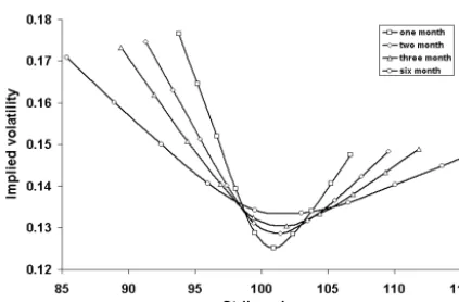
Figure 8: Sample-implied volatility surface generated by Willow smile model

Figure 8 shows a sample-implied volatility sur-face generated by the Willow smile/skew model that allows volatility to be state, as well as time, dependent as in the model of Dupire (1994). Such models are used when the Black-Scholes assumption of geometric Brownian motion does not hold, but the modeller wishes to avoid intro-ducing extra factors into the model. In the smile/ skew version of the Willow tree, the placement of the nodes is adjusted parametrically in order to induce a state-dependent volatility. The model is parametrized by a smile parameter, a skew parameter and a parameter that governs how fast the smile/skew fades with time. While parsimonious, this parametrization allows for a wide variety of surfaces, and fits data from mar-kets extremely well. Adopting a parametric approach yields other advantages such as stabil-ity and fast calibration to both European and American options.

Note that we need not rerun the linear programs in order to create the Willow smile model. The adjustments required to the node placement and transition probabilities can be done in real-time. Another example of such an extension is the two-factor convertible bond model, where the drift of the stock price is equal to the prevailing short rate, and the corresponding adjustment is applied to the stock price drift at each node in the tree to keep the model arbitrage free.

Figure 9: Typical convergence behavior of Willow barrier model

Barriers in the Willow tree are handled in a unique and flexible way. The tree is constructed of a set of “compound” time steps, each consist-ing of several sub-time steps. The probability of a knock-in or knock-out over a compound time step is determined using a Brownian bridge com-putation. (A Brownian bridge is a Brownian motion conditioned on fixed, initial and final time points.) This computation is performed over several sub-time steps so that the process more closely resembles a Brownian motion, making the use of the Brownian bridge analyti-cal results more appropriate. Figure 9 shows how convergence is enhanced by applying the Brownian bridge computation over more and more sub-time steps.

This approach to barrier options allows for time-dependent barriers as well as time- and state- dependent volatility. This method gives far greater modelling flexibility than the standard method of arranging a row of nodes to fall on the barrier.

Concluding remarks

extremely efficient improvement over such stan-dard trees, and one that also provides the flexi-bility for a wide variety of processes and models. The particular advantages of the Willow tree are vastly improved convergence of derivative prices and greeks, as well as superior stability. The Wil-low tree also gives complete freedom in choosing time steps, which simplifies the implementation of pricing models. Variations of the basic Willow tree model admit state-dependent volatilities in single- and multifactor models, and efficient and flexible computation of all types of barrier options.

Acknowledgements

The author wishes to thank Hans Beumé and Mark Davis for helpful conversations, and Frank Mao and Zhengyun Hu for superb programming and analytical support.

References

Curran, M., 1994, “Strata Gems,” Risk, 7(3):

70–71, March.

Dupire, B., 1994, “Pricing with a Smile,” Risk, 7(1): 18–20, January.

Hull, J., 2000, Options, Futures, and Other

Derivatives, Fourth edition, Toronto, ON: Prentice-Hall International, Inc.

Nelson, D., and K. Ramaswamy, 1990, “Simple binomial processes as diffusion

approximations in financial models,” Review of

Financial Studies, 3(3):393–430.

Press, W., S. Teukolsky, W. Vetterling and B.

Flannery, 1992, Numerical Recipes in C,

Second edition, Cambridge, Cambridge University Press.

Schmidt, W., 1997, “On a general class of one- factor models for the term structure of

interest rates,” Finance and Stochastics, 1(1):