in the Presence of Temporal Logic Specifications
Thesis by
Scott C. Livingston
In Partial Fulfillment of the Requirements for the Degree of
Doctor of Philosophy
California Institute of Technology Pasadena, California, USA
2016
c
2016
Acknowledgments
I have had the joy of being mentored by Richard M. Murray and Joel W. Burdick, both of whom have repeatedly provided me with good ideas, insight, and feedback. Their styles of working are refreshingly distinct. As my official adviser, Richard main-tains an unusual (well, perhaps usual at Caltech) multi-disciplinary group that has allowed me to easily and simultaneously pursue such diverse topics as code genera-tion for flight software at the Jet Propulsion Lab and lab automagenera-tion in synthetic biology. Since I arrived at Caltech in 2010, I have met many interesting members of Richard’s group, Joel’s group, and others in Control and Dynamical Systems, the CMS Department, and Caltech broadly. Many of these encounters have led to on-going collaborations, all of which I joyously acknowledge. Within the scope of this dissertation, I want in particular to thank Pavithra Prabhakar and Eric M. Wolff for inspiration and discussion. Ioannis Filippidis provided me with several useful comments about organization and preliminaries.
I also wish to thank Gerard J. Holzmann and Pietro Perona, who served both on my candidacy and thesis committees, and who have provided thorough and useful criticism of my work, as well as good ideas for future work.
Abstract
Contents
Acknowledgments iv
Abstract v
1 Introduction 1
1.1 Advent of verification and formal synthesis for robotics . . . 1
1.2 Topics and contributions of the thesis . . . 4
1.3 Novelty and related work . . . 9
2 Preliminaries 12 2.1 Formal languages . . . 12
2.2 Linear-time temporal logic . . . 14
2.3 The basic synthesis problem . . . 16
2.4 The modal µ-calculus . . . 17
2.5 Reactivity, games, and another basic synthesis problem . . . 19
2.6 Finite representations of dynamical systems . . . 22
3 Patching for Changes in Reachability 24 3.1 Introduction . . . 24
3.2 The game graph of a GR(1) specification . . . 24
3.3 Problem statement . . . 26
3.4 Strategy automata . . . 26
3.5 Synthesis for GR(1) as a fixed-point computation . . . 32
3.7 Reachability games . . . 37
3.8 Game changes that affect a strategy . . . 40
3.9 Algorithm for patching between goal states . . . 42
3.9.1 Overview . . . 42
3.9.2 Formal statement . . . 43
3.10 Algorithm for patching across goal states . . . 44
3.11 Analysis . . . 50
3.12 Numerical experiments . . . 52
3.12.1 Gridworlds . . . 52
3.12.2 Random graphs in Euclidean space . . . 56
4 Patching for Changes in Requirements of Liveness 61 4.1 Introduction . . . 61
4.2 Problem statements . . . 62
4.3 Adding goals . . . 64
4.3.1 Overview . . . 64
4.3.2 Algorithm . . . 67
4.3.3 Results . . . 70
4.4 Removing goals . . . 73
4.4.1 Overview . . . 73
4.4.2 Algorithm . . . 74
4.4.3 Results . . . 75
4.5 Numerical experiments . . . 76
4.5.1 Gridworlds . . . 77
4.5.2 Random graphs in Euclidean space . . . 77
5 Cross-entropy Motion Planning for LTL Specifications 82 5.1 Introduction . . . 82
5.2 Control system model and problem formulation . . . 83
5.2.1 Dynamics and labeling of states . . . 83
5.3 The basic CE-LTL algorithm . . . 84
5.3.1 Brief introduction to the cross-entropy method . . . 85
5.3.2 Representation of trajectories . . . 87
5.3.3 Deciding feasibility of trajectories . . . 88
5.3.4 Algorithm . . . 90
5.4 Relaxations of the basic method . . . 91
5.4.1 Incrementally restrictive LTL formulae from templates . . . . 92
5.4.2 Incrementally restrictive ω-automata . . . 94
5.5 Numerical experiments . . . 96
5.5.1 Dynamical systems and representations . . . 96
5.5.2 Comparisons among the basic method and relaxations . . . 100
5.5.3 Comparison with related work . . . 105
6 Conclusion 108 6.1 Summary and limitations . . . 108
6.2 Future work . . . 110
A Time semantics for two-player games 112 B Probability theory 115 C Implementation details 117 C.1 Introduction . . . 117
C.2 Incremental control for GR(1) games . . . 117
C.2.1 Code for an example . . . 119
C.2.2 Representing variables of other types as atomic propositions . 119 C.3 CE-LTL and relaxations . . . 120
Chapter 1
Introduction
1.1
Advent of verification and formal synthesis for
robotics
such as C, etc.
New notation is not progress unless there are significant theoretical results or practical tools that use it. For computer-aided verification, there have been in both respects. During the past 30 years, there has been great progress in the characteriza-tion of fundamental problems, e.g., determinacy of parity games, in the development data structures and methods for verifying concurrent software systems, e.g., ordered binary decision diagrams and techniques for SAT solving, and in the available tools for verification, e.g., the Spin model checker. A brief summary of the history of verification and formal logic until around the year 2003 can be found in [55].
While methods of verification demonstrate certain properties about a given sys-tem, methods of synthesis construct new systems that realize desired properties. In the context of theoretical computer science, “synthesis” tends to refer to the construc-tion of finite-memory policies of acconstruc-tion selecconstruc-tion for finite transiconstruc-tion systems (defined in Chapter 2), which are often regarded as modeling concurrent software processes, especially those that are non-terminating [4]. An early formulation of several syn-thesis problems in terms of predicates on input and output sequences was given in 1962 by Church [14]. However, it is only recently that practically useful algorithms have begun to be proposed and that specification languages admitting tractable de-cision procedures or good heuristics have been presented. In control theory, the term “synthesis” is less common, but one of the basic themes is exactly that of con-structing controllers that cause trajectories of a dynamical system to meet certain constraints and be robust or optimal according to some objective. In contrast to the setting studied in theoretical computer science, these systems may have state spaces that are differentiable manifolds and may have uncountable time domains (so-called continuous-time systems).
of hybrid dynamics. Despite the presence of unified or common notation, hybrid systems can exhibit behaviors that are absent in purely discrete or continuously-valued systems. Therefore new methods of analysis for verification and control have been developed for various kinds of hybrid systems [10, 25]. In summary, hybrid systems are especially challenging to control, and many negative results of undecidability or intractability have been proven [9, 35]. Much current research in the theory of hybrid systems is devoted to finding hybrid dynamics and specification languages that are interesting and have tractable control problems or approximations thereof. As well, developing notions of equivalence, reductions, and simulations are important topics of current work toward synthesis of controllers for difficult problems in this area.
At the same time as the aforementioned developments were made, there has been much progress in robotics research for motion planning. The basic problem concerns moving a rigid body from one point to another in a space among obstacles while avoiding collisions. Solving it precisely is known to be intractable [52]. As such, algorithms that provide exact solutions tend to rely on special structure, such as polygons with single-integrator dynamics navigating among a set of other polygons. In the presence of nonlinear dynamics and, in particular, nonholonomic constraints as occurring in car-like models, techniques of geometric control theory have yielded fast planners. While the point-to-point motion planning problem only requires particu-lar trajectories, practical issues like measurement noise and actuation disturbances have motivated methods based on reference trajectory tracking or potential functions. Another broad and important category that has practically been a great success is sampling-based methods, e.g., Probabilistic Road-Map (PRM) or Rapidly-exploring Random Trees (RRT) [36, 38]. Recently, sampling-based point-to-point kinodynamic planners have been proposed that are optimal, in a probabilistic convergence sense [29, 33].
the motion are relatively simple when considered as being part of some task or mission. For example, a surveillance robot must repeatedly move around a building, providing a certain amount of coverage, and respond to surprise requests, while periodically stopping at a battery-charging station, subject to hard time constraints because the battery must not become empty before reaching the station. Part of realizing this task involves solving point-to-point motion planning problems. Solutions for the task itself have historically been the product of manual design by humans, sometimes following templates for robot architectures. Algorithms for planning from research in artificial intelligence may be used at more abstract levels, such as A* for navigating a semantic map of the building, e.g., a graph where vertices represent rooms. However, the composition of various planning modules or the relation of outcomes from trajectory generation and tracking to the finite-state machine that guides task completion have historically been manually designed without techniques of formal verification, with which this section began, being applied.
Motivated by more automation while providing guarantees about correctness for task performance and completion, since around 25 years ago [12, 45, 51, 59], and beginning more intensely 9 years ago (e.g., [6, 16]), attention has been devoted to formally verifying robot architectures and synthesizing solutions to tasks. It should be apparent that this essentially recovers problems of verification and synthesis for hybrid systems, but now with an orientation toward systems and tasks that are of particular interest in robotics.
1.2
Topics and contributions of the thesis
Chapter 2 is dedicated to introducing preliminary background material in preparation for the main work of the thesis. Some detail can be found there about terms used here to summarize the topics and contributions.
demon-strations are widely valued in the robotics community. Anecdotal interactions by the author of this thesis with people who work on other topics of robotics indicate skepticism of the actual significance of publications about so-called formal methods for robotics. The importance of the ambitions is usually easily recognized. How-ever, there have been very few meaningful physical experiments, and most proposed methods rely on strong assumptions, e.g., control for systems that have trivial single-integrator dynamics, the absence of actuator uncertainty, or perfect knowledge of global position. With enough of these assumptions, it is possible to exactly recover the setting already treated in theoretical computer science, allowing the disappointing occurrence of papers that do little more than re-hash old ideas in a new venue.
Two important features of most problems in robotics are uncertainty and dynam-ics. These span the (artificial but often made) boundary between perception and control. Uncertainty essentially causes two fundamental problems in mobile robotics: mapping and localization. More broadly, uncertainty manifests from sensor noise, in-put disturbances, actuator failures, clock drift, lossy communication channels, object detection and tracking, among many other examples. Dynamics can be thought of as a feature of many problems in robotics because motion is always occurring or soon to occur, and the interplay of mechanics with software control is endemic. Obviously these features are not separate, e.g., disparity between a simplified model of dynamics and the physical hardware can be a source of uncertainty.
Addressing uncertainty and dynamics demands limiting or removing assumptions like perfect position information, known and fixed workspaces, and trivial dynamics. It is a premise of the thesis that they are important targets for research in formal methods for robotics. A sketch of the proposed program of research is to revisit previously well-studied cases of uncertainty in robotics, both in terms of specific sources like sensor noise and in terms of specific problems like localization, in the context of formal synthesis. Similarly, methods should specifically address the various major kinds of dynamics that are well known in robotics: differential drive, car-like dynamics, multi-link arms, dexterous manipulation, etc.
C
P
1 2
3 4 5
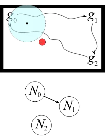
Figure 1.1: Illustration of the form of controllers developed in this thesis, shown in the context of a basic feedback loop. The arrows connecting the boxes are indicative of relationships and the directions of signals. They do not correspond exactly with inputs and outputs.
both of these features. Two problem settings are considered, each involving a broad category of synthesis: reactive and non-reactive (or closed-system). The first set-ting is essentially formulated as a game for which a finite-memory strategy must be constructed so as to ensure that a specification is satisfied despite an adversarial en-vironment. The specification is written in a fragment of linear-time temporal logic (LTL) referred to as GR(1). The game and strategy are finite structures, i.e., can be regarded as finite directed graphs together with a semantics of execution, turn-taking, and labels of atomic propositions. The problem of synthesis in this setting relies on the existence of a finite representation of a continuously-valued or hybrid dynamical system. Thus the winning strategy that is thought to realize the GR(1) specification is only one part of a controller that also generates trajectories of a plant, as illustrated in Figure 1.1. The relationship between plays in the GR(1) game and trajectories of the plant is made precise using a bisimulation, which is also referred to here as a discrete abstraction to emphasize that one side of the bisimulation equivalence is a transition system with finitely many states.
tran-sitioned to, and the subset of these transitions that are safe depend on the current move of an adversarial environment. The first major contribution of the thesis is to present algorithms for modifying strategies in the presence of changes to transition rules, i.e., changes to reachability in the GR(1) game. The problem and proposed solutions are described as incremental control synthesis because the changes are re-garded as occurring sequentially, and so the modifications to strategies so that they are winning with respect to the sequence occur incrementally. As part of the de-velopment of solutions in Chapter 3, an annotation for strategies in GR(1) games is presented that is crucial in ensuring that the results of patching are winning (i.e., correct with respect to the modified GR(1) specification). A variety of properties about the annotation is proven, and it is expected to be of interest independent from the incremental synthesis algorithms presented in the thesis.
Part of Chapter 3 is based on [43]. The basic idea of “patching” to recover cor-rectness after a change in workspace reachability was first presented in [42]. The algorithm developed there treats GR(1) synthesis as an opaque subroutine that is invoked to solve restricted specifications based on a subset of the state space and in-cluding the changed transition rules, which imply changes to reachability. Solutions of these are modified and then used to patch the original strategy. The methods in Chapter 3 rely on solving a game of lower computational complexity than GR(1) and so are favored to the algorithm of [42]. Though not developed further here, the opaque approach to patching is potentially easily extended to other classes of specifi-cations because the corresponding synthesis algorithms do not need to be revised or decomposed.
The problems posed in Chapters 3 and 4 all begin with a GR(1) formula ϕ that is modified to yield a new GR(1) formula. The basic practical motivation is that ϕ is known ahead of time and thus can be solved without significant time constraints. However, details may be missing or the model of motion at the abstract level of the game may have errors. During execution, observations from sensor data or news from a human operator that affects the task can imply modifications toϕ. Taken together, the solutions presented in Chapters 3 and 4 are sufficient to handle all substantial respects in which ϕ (and correspondingly, the game) could thus change, with the exception of changes to assumptions about environment liveness. The only other part of the GR(1) formula template is the initial conditions. Modifications to initial conditions do not affect the play currently in progress (recall the motivation of online changes occurring), and in any case, new initial states are easily handled as solutions to reachability games that are introduced in Chapter 3.
The methods for incremental control synthesis amidst changes to GR(1) formu-lae address more than uncertainty in task specifications. Recall that the synthesized strategy is interpreted as being part of a controller that drives a plant, possibly in-volving hybrid dynamics. In practice, the GR(1) game is not only an expression of desired behavior but also constraints among reachable regions, which in turn depend on a cell decomposition of the state space, or on the capabilities for trajectory gener-ation for driving a vehicle among cells. As such, refining the partition can manifest as new transition rules in the GR(1) formula, at which level the presented algorithms are relevant.
how to leverage BDDs with them.
The second problem setting studied in this thesis is that of non-reactive (or open-loop) trajectory generation for nonlinear systems. Whereas in previous chapters the problem setting requires finite decompositions and the existence of discrete abstrac-tions, Chapter 5 presents methods for stochastic optimization of trajectories of a nonlinear system that satisfy an LTL formula and minimize an objective function, all without construction of an abstraction. Furthermore, the labeling of states (in terms of which satisfaction of LTL formulae is defined) does not need to be expressed as unions of polytopes. The proposed algorithm is based on the cross-entropy method. As with any technique for stochastic optimization, obtaining good convergence per-formance is a key challenge, and to that end, several relaxations (heuristics) of the basic algorithim are also given. Chapter 5 is based on [44].
1.3
Novelty and related work
modified during execution, so is conservative in the sense that not all disturbances may occur.
The broad notion of incremental or on-the-fly methods for synthesis is certainly not novel, and it also occurs in the context of model checking [5, 22, 24, 56, 60]. However, the interpretation of the terms “incremental” and “on-the-fly” is in ref-erence to construction of the transition system that is to be controlled. Usually a method is called “on-the-fly” if the solution can be obtained without constructing the transition system entirely, whether symbolically (i.e., in a representation in terms of sets of states) or enumeratively (i.e., in a representation in terms of individual states). Solutions for the reachability games introduced in §3.7 could be obtained in an “on-the-fly” manner.
Methods for so-called strategy improvement are relevant insofar as it follows the present theme of incrementally modifying a game strategy. As suggested by “im-provement,” problems in that area of work concern optimization with respect to an objective. Roughly, the solutions are obtained in steps by beginning with some winning strategy and then modifying particular moves taken under it so that cost is reduced while remaining winning in the original parity game [54] (and references therein). The game itself does not change, and a strategy continues to be winning independently of the cost function.
Analogous to strategy improvement in the literature on theoretical computer sci-ence is so-called anytime algorithms in the AI and planning literature. The basic theme of anytime planning algorithms is to quickly present a feasible plan (or tra-jectory, or path, in the context of robotics) and then to improve it as much as time allows [34, 39]. Again, there is no change to the space of feasible solutions. However, there is some relevance in analogy, e.g., if the cost function is slowly changing during time, an anytime algorithm might be able to track the changes.
Obviously this does not solve the problem but merely translates it to a different level. The abstraction thus provides a crucial interface, and there are methods for refining it as needed based on counter-examples [1]. Such work is relevant insofar as it provides a way to cope with uncertainty by preventing its inclusion in the abstracted system. It can thus also be regarded as complementary to the methods in Chapters 3 and 4. Recently there has been work in robotics considering formal synthesis for specifi-cations expressed in LTL and GR(1) and in the presence of uncertainty or incremental controller construction [23, 53, 61, 65, 67]. A broad organization of this work is pos-sible according to whether it is reactive (in the sense of a game; cf. §2.5) and where uncertainty occurs: in the dynamical system modeling the robot, in the environment or workspace, or in the temporal logic formulae providing the task specification. Ob-viously there is some overlap among these, and indeed, a question for research is how to trade-off uncertainty among them, possibly as a design choice using abstraction refinement as suggested above.
Chapter 2
Preliminaries
In this chapter, preliminary developments are made in preparation for the main work of the thesis. Besides fixing notation, this chapter also serves to very briefly provide background material appropriate for a general audience who is broadly familiar with control and dynamical systems but not necessarily with the specific topics prerequisite for this thesis. Additional preparatory notes for a more general audience are given in the appendices.
Before beginning, some basic notation is introduced. The set of real numbers is
R (it is also sometimes referred to as the real line), the set of integers is Z, and the
set of positive integers isZ+. The natural numbers begin at 0 (and thus are equal as
a set to the nonnegative integers) and are denoted by N. Let A and B be sets. The set of all subsets of A is denoted by 2A. The set of elements in A but not in B (i.e., the set difference) is A\B.
A closed interval of the real line is denoted by [a, b], where a≤b and a and b are known as endpoints. An open interval with the same endpoints is denoted by ]a, b[.
2.1
Formal languages
Let Σ be a finite set. A finite string of Σ is a function σ :{0,1, . . . , n} →Σ, where n ∈ N. When there is no ambiguity about the set Σ, we simply refer to σ as a
Let α : {0,1, . . . , n} → Σ and β : {0,1, . . . , m} → Σ be strings. Define an operation, denoted by αβ (i.e., by juxtaposition) and called concatenation, that is defined as the function
αβ(t) =
α(t) if 0≤t ≤n β(t−n−1) otherwise,
(2.1)
where 0 ≤ t ≤ n+m+ 1. It is immediate that αβ is a finite string and has length n+m+ 2. The set of all finite strings of Σ is denoted by Σ+. A language is a subset
of Σ+.
After adding an empty string to Σ+ (as an identity element under the
concatena-tion operaconcatena-tion, and thereby obtaining the Kleene closure Σ∗), we have the basis for studying regular languages, context-free grammars, etc., which are outside the scope of this preliminaries chapter. Interested readers should begin at [26].
Most of the specifications considered in this thesis are for nonterminating systems, i.e., having trajectories of infinite duration. As such, we are also interested in strings that have countably infinite length. An infinite string of Σ is a function σ :N→Σ. When there is no ambiguity about the set Σ, we simply refer toσas aninfinite string. The set of all infinite strings of Σ is denoted by Σω. When the distinction between
infinite or finite string is without consequence, or if a property holds in both cases, we simply write string. Concatenation as in equation (2.1) is defined between finite strings and infinite strings, in that order, where they are also referred to asprefix and
suffix, respectively.
Let σ be a string. A substring of σ is a string obtained by restricting the domain of σ and shifting indices to begin at 0. Precisely, let I be an interval of the form [a,∞[ or [a, b], where a, b∈N, 0 ≤a ≤b, and b is less than the length of σ if σ is a finite string. Define σI(t) = σ(t+a), where ifI = [a, b] then t can take value at most
2.2
Linear-time temporal logic
Since its introduction as a formalism for specifying properties of programs by Pnueli in 1977 [49], linear-time temporal logic (LTL)1 has enjoyed widespread adoption and
has been the subject of and used in much research. There are many variants and details that can be considered [20], but only the basic propositional construction is used here. General introductions can be found in [4, 15].
As for any specification language, LTL is defined in two parts. First, the syntax determines the notation by defining the formulae that can possibly be written. Sec-ond, the semantics are defined in terms of string containment, thus determining when a sequence can be said to satisfy an LTL formula. Before beginning, we introduce the main device of labelings. Let AP be a set of atomic propositions. For readers who are familiar with programming languages like C++ and Python, atomic propositions can be thought of as variables of type bool and are thus able to take one of two values: true or false. More generally, they are the basic (indivisible, i.e., atomic) units of truth-value. States of a dynamical system are labeled according to whether each atomic proposition in AP istrueorfalseat that state. The labeling is given or otherwise chosen and thus not usually a part of the control synthesis problem; rather, synthesis is described as a problem about realizing certain sequences of truth-values of atomic propositions.
In this thesis, the set-theoretic style is used, wherein each subset B ⊆ AP is interpreted as an assignment of true and false to atomic propositions according to presence in or absence from B, respectively. Explicitly, p is true if and only if p∈B. Because subsets correspond to assignment of values, they are also referred to asstates. (Thus, B ⊆AP is a state, and 2AP is a set of states.) In terms of variables taking values on finite domains, development in terms only of atomic propositions is without loss of generality because any such variable admits a binary representation; cf. §C.2.2.
The syntax of LTL is described as a context-free grammar. In Backus-Nauer form,
1LTL is also known as “linear temporal logic.” Here the former is preferred to emphasize that
the production rules are
ϕ::= p| ¬ϕ|ϕ∨ϕ| ϕ|ϕUϕ (2.2)
where p ∈ AP and ϕ is a nonterminal. The first three productions provide the familiar propositional (non-temporal) logic, sometimes called Boolean logic. The other productions introduce temporal operators. (The meaning of “temporal” will become apparent with the semantics as defined below.) From these, the following operators are syntactically derived:
• true≡p∨ ¬p
• ϕ∧ψ ≡ ¬(¬ϕ∨ ¬ψ)
• ϕ =⇒ ψ ≡ ¬ϕ∨ψ,
• ϕ ⇐⇒ ψ ≡(ϕ =⇒ ψ)∧(ψ =⇒ ϕ),
• ϕ≡trueUϕ,
• ϕ≡ ¬ ¬ϕ,
• false≡ ¬true.
Before proceeding to semantics, notice that among the productions in (2.2) there are no parentheses, i.e., the symbols ( and ). They are not considered a part of the syntax of LTL, but rather, they are used to emphasize precedence. As is conventional, an expression in parentheses is evaluated before any expression containing it. Parenthe-ses are applied to remove ambiguity about parsing an LTL formula, i.e., ambiguity about the sequence in which productions from (2.2) are applied, which affects the in-terpretation of the formula because the semantics are defined inductively on grammar productions.
Let ϕbe an LTL formula (having the syntax defined above). Letσ be an infinite string of 2AP, and lett ∈
σ, t|=ϕ, is defined inductively on the parse tree of ϕ(i.e., the grammar productions that yieldϕ) as follows.
• σ, t|=true;
• σ, t|=p if and only if p∈σ[t,∞[(0) (which is equivalent to p∈σ(t)); • σ, t|=¬ϕ if and only if σ, t|=ϕis not true, which is written σ, t6|=ϕ;
• σ, t|=ϕ if and only if σ, t+ 1 |=ϕ;
• σ, t|=ϕ if and only if for all τ ≥t,σ, τ |=ϕ;
• σ, t|= ϕif and only if there exists τ ≥t, σ, τ |=ϕ;
• σ, t|=ϕUψ if and only if σ, t|=ψ or there exists j >0 such that σ, t+j |=ψ and for all 0≤i < j, σ, t+i|=ϕ.
If σ,0 |= ϕ (i.e., t = 0), then we simply write σ |= ϕ. Several of the definitions are redundant but included for clarity, e.g., σ |= ϕ could be obtained using σ |=
trueUϕ, following the syntactic derivation given earlier.
2.3
The basic synthesis problem
Having introduced LTL as a language for expressing specifications, we need only introduce a structure that admits some notion of control in order to be able to pose a synthesis problem. A transition system is a tuple T = (S, I,Act,→, L,AP) where S is a set of states (not necessarily finite), I ⊆ S is a set of initial states, and
→⊆ S ×Act×S is a relation. States are labeled with the function L : S → 2AP.
This sketch of transition systems follows the literature [4, 58]. Precise problems are formulated in later chapters, but it is useful to provide a sketch of a basic synthesis problem here.
Problem 1 (sketch). Letϕ be an LTL formula in terms of the atomic propositions AP. Find a partial function C : S+×
N →Act such that all state sequences of the
2.4
The modal
µ
-calculus
A more expressive language than LTL, which was introduced in§2.2, isµ-calculus. In this section it is briefly introduced with a focus on only those parts relevant for this thesis. Applications and research involving µ-calculus are rich, and readers who are generally interested in it should consult [21, 55]. The primary motivation to introduce µ-calculus, despite working primarily with specifications that can be expressed in LTL, is that it readily admits so-called fixed-point algorithms that provide one basis for strategy synthesis. In particular, intermediate values provide sequences of sets of states that may be useful for reachability computations, as in§3.5.
Let AP be a set of atomic propositions, and let Var be a set of variables. A Kripke structure is a triple K = (S,R, L) where S is a finite set of states, R ⊆ S ×S is a relation, and L : S → 2AP is a function that labels each state with a set of atomic propositions that are true in that state. An execution of K is a sequence of states s : N → S such that (s(t), s(t + 1)) ∈ R for all t ≥ 0. The trace of an execution s is the function w : N → 2AP such that w(t) = L(s(t)) for t ≥ 0. An initial state
could also be defined as part of the Kripke structure, but it is not needed here. A transition system, as defined in §2.3, in which there are no control actions available is equivalent to a Kripke structure (after defining initial states).
Let X ∈ Var be a variable, and let Q ⊆ S be a set of states of the Kripke structure K. Define the new Kripke structure KQX = (S,R, L0) over the set of atomic propositions AP0 = AP∪{X } and where
L0(s) =
(
L(s)∪ {X } if s∈Q L(s) otherwise.
The syntax of µ-calculus is defined by the following grammar productions.
φ::=p| X | φ∨φ| ¬φ | φ|φ |µX.φ|νX.φ
defined on Kripke structures. Observe that a trace of a Kripke structure is just an infinite string of 2AP, so the semantics of LTL can as well be defined on Kripke structures. Proceeding inductively on the syntax, we have
[[p]]K={s∈S |p∈L(s)}
[[φ∨ψ]]K= [[φ]]K∪[[ψ]]K
[[¬φ]]K=S\[[φ]]K
[[φ]]K={s∈S | ∀s0 ∈S.(s, s0)∈ R =⇒ s0 ∈[[φ]]K}
[[ φ]]K={s∈S | ∃s0 ∈S.(s, s0)∈ R ∧s0 ∈[[φ]]K}
Consider the recursion on subsets of S defined by
Q0 =∅
Qk+1 =Qk∪[[φ]]KQk
X .
It turns out that there is some k∗ where Qk∗+1 = Qk∗, i.e., it is a fixed-point under the function defined by [[φ]]KQ
X. [[µX. φ]]K is defined to be this set. Similarly, [[νX. φ]]K is defined inductively by
Q0 =S
Qk+1 =Qk∩[[φ]]KQk
X .
2.5
Reactivity, games, and another basic synthesis
problem
The adjective “reactive” is commonly used in robotics to refer to a style of control that, informally, lacks much foresight or planning. Instead, actions are selected based on superficial interpretations of sensor measurements. A small example is a thresh-olding routine that stops all motion if any range finder values are too small (and pre-sumably are indicative of potential collisions). The basic paradigm is demonstrated in the robot architectures broadly categorized as being behavior-based [13].
Following instead the convention in the theoretical computer science literature [50, 55], throughout this thesis the term reactive is used to indicate the presence of an adversary that selects values for some of the inputs. This is analogous to the notion of disturbance in robust control theory [18, 27]. However, using LTL as introduced in§2.2, we can express a time-varying dependence between disturbances (adversarial or uncontrolled inputs) and the states that should be reached by the controller. This situation can be described as a turn-based game, and the objective is to ensure that an LTL formula is satisfied, despite all possible adversarial strategies.
The intuitive sketch above is now made precise. Let AP be a set of atomic propo-sitions, and partition it into APenv and APsys. The former set contains atomic propo-sitions that take truth-value according to the choice of an adversary, i.e., they are uncontrolled and thus always present the possibility of the worst-case. The latter set, APsys, has propositions that we are able to control. Note that the control (assignment of values to) APsysmay only be indirect, e.g., after driving the state of the underlying dynamical system into some polytope, as described in§2.6.
The reactive synthesis problem for LTL is as follows. Let ϕbe an LTL formula in terms of APenv∪APsys. For any infinite string σenv of 2APenv, find an infinite string
σsys of 2APsys
such that the combination, defined as
for t≥0, and being a string of 2APenv∪APsys, satisfies ϕ. While this problem
formula-tion is attractive because it is consistent with the perspective of systems as funcformula-tions of entire input sequences to entire output sequences, there are obvious practical dif-ficulties.
Example 1. Let APenv ={p}, and let APsys={q}. The reactive LTL specification
q ⇐⇒ p
has only solutions that are not causal. Intuitively, the right-side of the formula is satisfied if for all time p istrue. However, the left-side is satisfied if q is trueat the initial state. Thus, this instance of the reactive synthesis problem requires a controller that can predict the value of p. Since the adversary decides the truth-value of p and has no constraints, this is practically impossible.
The reactive synthesis treated in this thesis is for a fragment of LTL known as GR(1) (generalized reactivity of rank 1, or generalized Streett[1]) [31]. Together with some conditions determining initial states (given below), GR(1) is syntactically defined by the formula template
ρenv∧
m−1
^
j=0
ψenvj
!
=⇒ ρsys∧
n−1
^
i=0
ψisys
!
, (2.3)
where each subformula is defined in terms of atomic propositions as follows. All ofψenv
j
andψsysi are formulae in terms of APenv∪APsys and without temporal operators. ρenv
is a formula in terms of APenv∪APsys and can only contain the temporal operator
in direct application to atomic propositions of APenv, i.e., only as subformulae
p where p ∈ APenv. Finally, ρsys is a formula in terms of APenv∪APsys and can
A play is an infinite sequence of subsets of APenv∪APsys, i.e., a function σ:N→
2APenv∪APsys, where at time t≥1, σ(t) is determined in two steps: 1. the environment selects a subset e ⊆APenv;
2. given e, the system selects a subsets ⊆APenv,
and then σ(t) = e∪s. This interpretation of turn-taking is known as a Mealy time semantics (cf. Appendix A). Keeping this in mind, a playσis simply an infinite string of Σ = 2APenv∪APsys, and as such, the notation defined in §2.2 for satisfaction of an LTL formula can be used, e.g., σ|=ϕ, where ϕis of the form (2.3).
A GR(1) game is a pair G = (ι, ϕ) where ϕ is of the form (2.3), ι ∈ Σ is the
initial state. A play σ is said to be initial if σ(0) = ι. An environment strategy is a function g : 2APenv∪APsys+ → 2APenv. A (system) strategy is a partial function f : 2APenv∪APsys+
× 2APenv → 2APsys. A play σ :
N → 2AP
env∪APsys
is said to be
consistent with environment strategy g and system strategy f if for all t≥0,
σ(t+ 1) =g(σ[0,t])∪f(σ[0,t], g(σ[0,t])). (2.4)
By the Mealy time semantics, the presence of g(σ[0,t]) as an argument of f is
well-defined. A system strategyf is said to bewinning if and only if for every environment strategy g and for every initial play σ that is consistent with f and g, σ |=ϕ.
Problem 2 (GR(1) synthesis). Let G = (ι, ϕ) be a GR(1) game. Find a system strategy f that is winning, or decide that one does not exist.
If a winning strategy exists, the GR(1) game G is said to be realizable. In this case, a winning strategy f is said to realize G. When the initial state does not need to be distinguished, for brevity we may only refer to a GR(1) game directly as the LTL formulaϕ.
While Problem 2 is in terms of a single initial state, there are several possibilities for deciding the initial states and, together withϕ, thereby defining the set of winning plays. The distinction is not crucial for this thesis. For completeness, three common choices are outlined here, all of which can be represented using the single initial state formulation given above, possibly after an appropriate modification to the transition rules. Let Init⊆2APenv∪APsys.
1. Plays can begin at any state in Init. The (adversarial) environment can arbi-trarily select it.
2. Plays begin at some state, which can be chosen along with the system strategy. 3. For each assignment of APenv (chosen by the environment), the system strategy
must choose an assignment of APsys such that the combined state is in Init. The definition of the GR(1) synthesis problem relies on the interpretation of plays as infinite strings. However, if a state transition occurs in whichρenv orρsysis violated,
then the play is decided (winning if the former is violated; not winning otherwise), and the remaining infinite string suffix is not relevant. In particular, a winning strategy could be one that forces the environment to violateρenv. Such winning strategies will not be addressed in this thesis. Indeed, because the suffix of a play is not relevant, a different problem can be posed as finite-time reachability, which is subsumed by reachability games that are posed and solved in §3.7.
The basic synthesis procedure for GR(1) is crucial for some of the development in
§3 and is outlined there in §3.5.
2.6
Finite representations of dynamical systems
taken in Chapter 5. Alternatively, a finite transition system may be constructed that preserves appropriate aspects of the original system, i.e., the physical system that we actually want to control. The relationship between these two systems is a simulation or bisimulation [2, 4, 40, 58]. There are many possibilities for achieving this, and indeed, construction of and control for abstractions is a topic of current research. Im-portant extensions have also been proposed, including probabilistic and approximate bisimulations.
Basic ingredients are illustrated by the approach taken in [66], where in summary the state space for a piecewise linear system is partitioned into finitely many polytopes that refine labeling of states in terms of atomic propositions. Abstraction construction involves checking, for each pair of cells, whether it is possible to reach one from any state in the other, using a fixed or varying number of states and allowing for disturbances. Because regions are polytopes and the dynamics are linear, it is possible to pose this as feasibility checking in a linear program. The existence of a feasible point implies the existence of a control sequence from one cell to another. The abstract system is then a directed graph with vertices corresponding to polytopes and edges corresponding to the existence of feasible points, i.e., of input sequences from one cell to the other.
Chapter 3
Patching for Changes in
Reachability
3.1
Introduction
A fundamental problem for dynamical systems is determination of the reachable state space. The construction and analysis of controllers essentially involves controlling the reachable states and the manner in which they are reached, e.g., manifesting for linear systems as basic parameters like rise and settling times [3].
The intuitive setting for this chapter is one in which we have already considered the reachable state space and constructed a controller that satisfies an objective in it. A game is being played against the environment and so the controller is, in part, a strategy that is winning in terms of that game. If some of the possible transitions in the game are changed, what can we do with the nominal strategy that we already have? Obviously it is always an option to discard it and construct another strategy de novo, but in some situations we can do better. This sketch is made into a precise problem in this chapter, and a solution for it is developed. Parts of this chapter are based on joint work with Prabhakar [43].
3.2
The game graph of a GR(1) specification
APsys. For conciseness, let Σ = 2APenv∪APsys. Throughout the chapter, elements of Σ,
i.e., subsets of APenv and APsys, will be written as lowercase letters such as x. This convention is to emphasize the perspective of assignments of truth-values to atomic propositions as states.
Here and in the next chapter, it will be useful to think of plays in terms of infinite-length walks on a graph obtained from the safety subformulae, ρenv and ρsys, of ϕ. Before defining the graph obtained from ϕ, the notation for satisfaction developed for LTL in§2.2 is extended slightly to provide for transition rules. Let x, y ∈Σ. For ρ ∈ {ρenv, ρsys}, define (x, y) |= ρ as the predicate: for every infinite string σ of Σ
such that σ(0) = x and σ(1) =y, σ |= ρ. Intuitively, (x, y) |= ρ holds if and only if every infinite string that has first element xand second element y satisfies ρ. This is useful because, as defined in §2.5, the only temporal operator that can appear in ρis
, and it can only be in a subformula of the form p for an atomic proposition p. Thus, satisfaction of it by any infinite string can be decided using only the first two elements. Similarly, for a formula without temporal operators θ, define x|=θ if and only if σ |=θ for every infinite string σ of Σ such that σ(0) =x. (The restriction of θ lacking temporal operators could be removed, but the generality is not needed.)
Define the graphGϕ = (Σ, Eϕenv, Eϕsys), where Σ is as defined earlier, and forx∈Σ
and y⊆APenv,
Eϕenv(x) ={z ⊆APenv |(x, z)|=ρenv}, (3.1) Eϕsys(x, y) ={z ⊆APsys|(x, y∪z)|=ρsys}. (3.2)
Gϕ is a directed graph in that Eϕenv and Eϕsys together provide an edge set, namely
(x, y) ∈ Σ ×Σ is an edge if and only if y ∩ APenv ∈ Eϕenv(x) and y ∩ APsys ∈
Esys
ϕ (x, y ∩AP
env). This definition deviates from the usual definition of game graph
3.3
Problem statement
Recall the template for GR(1) formulae (2.3) from §2.5,
ρenv∧
m−1
^
j=0
ψjenv
!
=⇒ ρsys∧
n−1
^
i=0
ψisys
!
.
Problem 3. Let ϕ0, ϕ1, . . . be an infinite sequence of GR(1) formulae that all have
the same subformulaeψenv
j , j = 0, . . . , m−1, andψ
sys
i ,i= 0, . . . , n−1, but possibly
distinct transition rules, i.e., the sequence of GR(1) formulae is characterized by a sequence of pairs of formulae
(ρenv0 , ρsys0 ),(ρenv1 , ρsys1 ), . . . . (3.3)
Find a sequence of strategies f0, f1, . . . such that fk realizes ϕk, the formula having
ρenvk and ρsysk .
The statement as given does not address causality, i.e., whether the entire sequence of specifications is known at once or given incrementally. Practically motivated, we consider the latter, but the proposed solution could as well be used for the former.
3.4
Strategy automata
The definition of strategy given for reactive synthesis allows, in general, dependence on the entire history of a play (cf. §2.5). For GR(1), a finite-memory suffices [31]. In this section, the particular form of finite-memory strategy used in this thesis is defined. (Because only finite memory is required, these strategies are also generically referred to as “finite-state machines.” To avoid confusion with the many variants of usage for that term, it is avoided here.)
Let ϕ be a GR(1) formula as in (2.3), and let Σ = 2APenv∪APsys. A strategy
game states, and δ is a function that determines successor nodes in A given inputs from the environment, i.e., valuations represented as subsets of APenv, so that state transitions are consistent with ρenv and ρsys. The domain of δ is
[
v∈V
{v} ×Eϕenv(L(v)),
and for every v ∈V, e∈Eenv
ϕ (L(v)), L(δ(v, e))∩AP
env =e and (L(v), L(δ(v, e)))|=
ρsys(so, L(δ(v, e))∩APsys∈Eϕsys(L(v), e)). Intuitively, the domain of δensures that a transition exists for each possible move by the environment from each state that can occur in A, and the game state labeling the node that is obtained after the transition is required to be consistent, i.e., the uncontrolled part of the state (in APenv) is the same as that which enabled the transition leading there, and the labels of node and predecessor together are feasible among available system (robot) moves.
Example 2. Let APenv = {door open,door reached} and APsys = {goto door}. Consider the GR(1) formula having
ψ0env = (goto door →door reached)
ρsys= (door open → goto door)∧((goto door∧ ¬door reached)→ goto door) ψ0sys=door reached,
which encodes the task of going to a door whenever it becomes open. (The left-side of each equality corresponds with a subformula of (2.3).) If the door is detected as open (as in the left subformula of ρsys), then the robot transitions into the mode of
goto door. It cannot leave that mode until the door is reached, which is indicated by the atomic proposition door reached. The environment can declare when it is reached and when it is open. The only liveness condition assumed to be satisfied by the environment, (goto door→door reached), can be thought of as providing a fairness assumption. If the robot continues to try to go to the door, eventually it will be reached.
7; (0, 1)
{}
0; (0, 1) door_open 6;
(0, 1) goto_door
2; (0, 0) door_reached, goto_door
4; (0, 1) door_open, goto_door 1;
(0, 0)
door_open, door_reached, goto_door
5; (0, 0) door_reached
[image:36.612.157.490.97.564.2]3; (0, 0) door_open, door_reached
Figure 3.1: A winning strategy automaton for the GR(1) game of Example 2. Each node has three rows. The first row contains an integer that uniquely identifies the node. The second row is a pair of values that is part of a reach annotation for the strategy (defined later in§3.6). Third is the set of atomic propositions that are true
In §2.5, GR(1) games are defined as having a single initial state. Therefore, it suffices to always consider a strategy automaton with a singleton set of initial nodes, I ={v0}. As discussed there, other interpretations of initial conditions can be
recovered with appropriate modification of the set of states Σ or the transition rules ρenv and ρsys. Other initial conditions could be treated by having more initial nodes
in the strategy automaton, without having to construct an equivalent game with one initial state.
Let A = (V, I, δ, L) be a strategy automaton. The graph associated with A has edge setE(A) determined by enumerating possible adversarial inputs from each node, i.e.,
E(A) ={(u, v)∈V ×V | ∃x⊆APenv. δ(u, x) =v}. (3.4) As a directed graph (V, E(A)) the usual notation can be applied. For any node v ∈ V, the set of successors of v is denoted by Post(v) = {u ∈ V | (v, u) ∈ E(A)}, and similarly the set of predecessors of v is denoted by Pre(v). An execution of A is a function r : N → V such that (r(t), r(t+ 1)) ∈ E(A) for t ≥ 0, and r(0) ∈ I. The trace associated with the execution r is the function L(r) : N → Σ defined by
in Eenv
ϕ (L(v)) during an execution that reached node v, then δ is not defined.
How-ever, the play is immediately winning, so the strategy automaton can be ignored. Furthermore, from the definition of strategy automaton, it is not possible to reach a state where Eϕsys(L(v), e) is empty, i.e., where there are no safe system (robot) moves from the node v given the permissible environment move e. Such a strategy could not be winning because there would be at least one play in which the environment (adversary) drives the game to an unsafe state. Besides these reasons, encoding safe transitions directly into the definition is well motivated because it aligns with the parity game perspective, in which the safety (transition) formulae ρenv and ρsys are
represented instead as edges in a game graph (cf. §3.2 and Appendix A).
Definition 1. Let (ι, ϕ) be a GR(1) game, and let A = (V,{v0}, δ, L) be a strategy
automaton for it. Let./be an arbitrary object that is not a node of A (i.e., ./ /∈V). For any g :N→2APenv, define the function ˆrg :
N→V ∪ {./} inductively as
ˆ rg(0) =
v0 if ι=L(v0)∧g(0) =ι∩APenv
./ otherwise
ˆ
rg(t+ 1) =
δ(ˆrg(t), g(t)) if ˆrg(t)∈V ∧g(t)∈Eϕenv(L(ˆrg(t))) ./ otherwise
fort∈N. Equivalently, define the function ˆr: 2APenv+
→V∪{./}as ˆr(g[0,t]) = ˆrg(t).
Finally, denote the projection of a string σ of 2APsys∪APenv onto APenv by
σenv(t) =σ(t)∩APenv
for t ≥ 0. Then, the strategy induced by A is the function fA : 2AP
env∪APsys+
×
2APenv →2APsys such that forσ ∈ 2APenv∪APsys+
and e∈2APenv,
fA(σ, e) =
L(ˆr(σenve))∩APsys if ˆr(σenve)6=./
∅ otherwise.
(3.5)
yields a strategy winning in the GR(1) game. Thus, it is enough to verify that a given strategy automaton is winning in order to solve a GR(1) game. (This result motivates the repeated use of “winning.”)
Theorem 1. Let A be a strategy automaton that is winning for a GR(1) game(ι, ϕ). Then the strategy induced by A is winning.
Proof. Let A= (V,{v0}, δ, L) be a winning strategy automaton for the GR(1) game (ι, ϕ). Let fA be the strategy induced by A. Let g : 2AP
env∪APsys+
→ 2APenv
be an environment strategy. The initial play σ consistent with fA and g is defined
inductively by
σ(0) =ι
σ(t+ 1) =g(σ[0,t])∪f(σ[0,t], g(σ[0,t]))
for t ≥ 0. In Definition 1, ˆr is defined on any finite string of 2APenv. Thus, from
equation (3.5),fA is defined on any finite string of 2AP
env∪APsys
and subset of APenv. Denoting projection ofσonto APenvbyσenvas in Definition 1, we have that ˆr(σenv
[0,τ]) =
./if and only if there is a positiveT ≤τ such that ˆrσenv
(T) =./and ˆrσenv
(t)∈V for t < T. (Observe that σ(0) =ι and L(v0) =ι by hypothesis, hence ˆrσ
env
(0) 6=./ and T > 0.) Therefore, σ(T −1)∩APenv 6∈Eenv
ϕ (L(ˆrσ
env
(T −1))), i.e., the environment move does not satisfy ρenv by definition of Eenv
ϕ . Because ˆrσ
env
(t) ∈ V for t < T, L(ˆrσenv
(t)), L(ˆrσenv
(t+ 1))
|= ρsys for t < T −1 by the definition of transitions (δ)
in strategy automata. Thus, the play satisfiesϕ. For the other case, i.e., ˆr(σenv [0,τ])6=./
for allτ ≥0, ˆrσenv
is an execution of A, soσ=L(ˆrσenv
) is a trace ofA. By hypothesis A is winning, hence σ|=ϕ.
3.5
Synthesis for GR(1) as a fixed-point
computa-tion
The basic method for synthesis outlined in this section is not a contribution of this thesis, e.g., it has been described earlier in [31] (and later as [8]), albeit with different notation. Nonetheless it plays a crucial role in the remainder of this chapter, so we are motivated to discuss it.
Before beginning, the setting is informally sketched. Intuitively, one manner of constructing a strategy that realizes (2.3) is to pursue states that satisfyψ0sysand from which it is possible to reach states satisfying each of the other liveness subformulae, ψ1sys, . . . , ψnsys−1. When this is not possible, there must be some way to block liveness of the environment, i.e., to eventually begin an infinite sequence of states in which ψenv
j
is not satisfied, for some j ∈ {0, . . . , m−1}. Provided environment liveness, upon reaching a state that satisfies ψ0sys, attention shifts to pursuing a state that satisfies ψ1sys, and the process continues. Because this superficially resembles a sequence of reachability problems on a finite graph, one may guess that a solution is obtained by repeated predecessor computations as familiar for shortest paths problems. However, an important difficulty is that each transition depends on the environment. In other words, the reactivity in this process is the presence of an adversary that, at each time step, can select an arbitrary valuation for part of the state. Thus, the solution is a strategy (not merely a walk on a graph), and the predecessor sets must quantify over possible moves by the environment.
The above sketch is now made precise. Let ϕbe a GR(1) formula as in (2.3), and recall the definition of the associated graph Gϕ given in§3.2. Let X ⊆Σ. The set of
controlled predecessors of X is defined by
Preϕ(X) =
y∈Σ| ∀z1 ∈Eϕenv(y).∃z2 ∈Eϕsys(y, z1). z1∪z2 ∈X . (3.6)
found using µ-calculus formulae
νZi. µY. m−1
_
j=0
νXj. (ψsysi ∧Preϕ(Zi+1))∨Preϕ(Y)∨ ¬ψjenv∧Preϕ(Xj)
!!
, (3.7) where the subscript addition of Zi+1 is modulo n (the number of system liveness
subformulae in (2.3)), and where i ∈ {0,1, . . . , n−1}. That is, the entire formula
Wϕ is a chain of subformulae, one (3.7) for each value of i. As outlined in §2.4,
Wϕ = [[Wϕ]] is obtained using a point computation. Moreover, at the
fixed-point, Wϕ =Z0 = [[Z0]] =Z1 =· · ·=Zn−1, and Wϕ = Preϕ(Wϕ).
Let i ∈ {0,1, . . . , n−1}. An intermediate value of the fixed-point computation used to obtain Wϕ is a finite sequence of sets
Yi0 ⊂Yi1 ⊂ · · · ⊂Yik=Wϕ, (3.8)
for some k, where Y0
i is a set of states in Wϕ that satisfies ψisys. Furthermore, for
eachl ∈ {1,2, . . . , k}, from every statex∈Yil, for allz ∈Eϕenv(x), at least one of the following holds:
1. there exists y∈Eϕsys(x, z) such that z∪y∈Yil−1, or
2. there is a strategy blocking one of the environment liveness conditions, ψenv
j ,
that remains within Yil.
Details about construction are given in [8, 31].
3.6
Annotating strategies
(patches). Note that the following definition was initially given in [41] and is modified from the earlier version of [43].
Let ϕ be a GR(1) formula as in (2.3). A state x ∈ Σ is said to be an i-system goal if x|=ψisys. Recall that Σ = 2APenv∪APsys.
Definition 2. A reach annotation on a strategy automaton A = (V, I, δ, L) for a GR(1) formula ϕ is a function RA : V → {0, . . . , n− 1} × N that satisfies the following conditions. Write RA(v) = (RA1(v),RA2(v)).
1. For each v ∈V, RA2(v) = 0 if and only if L(v) is a RA1(v)-system goal.
2. For each v ∈ V and u ∈ Post(v), if RA2(v) 6= 0, then RA1(v) = RA1(u) and
RA2(v)≥RA2(u).
3. For any finite executionv1, v2, . . . , vKofAsuch that RA2(v1) =· · ·= RA2(vK)>
0, there exists an environment goalψjenv such that for allk ∈ {1, . . . , K},L(vk)
does not satisfy ψenv
j .
4. For each v ∈ V and u ∈ Post(v), if RA2(v) = 0, then there exists a p such
that for all r between RA1(v) and p, L(v) is a r-system goal, and RA1(u) =
p. Specifically, if p < RA1(v), the numbers between p and RA1(v) are p+
1, . . . ,RA1(v)−1, and if RA1(v)≤p, then the numbers between pand RA1(v)
are p+ 1, . . . , n−1,0, . . . ,RA1(v)−1.
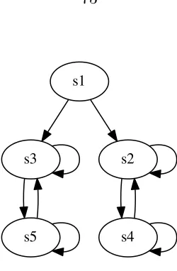
An illustration of a strategy automaton with a reach annotation on it is given in Figure 3.2. It realizes a deterministic (without adversarial environment) game. The strategy automaton shown earlier in Figure 3.1 as part of Example 2 provides a slightly more complicated demonstration of a reach annotation.
Remark 2. During basic synthesis, a reach annotation can be constructed using the indices of the intermediate values (Yl
i in (3.8)) of the fixed-point computation on
(1,1)
(1,0)
(0,1)
(0,2)
g0
g1
v0v1
v2
v3 v4 v5
(0,1)
[image:43.612.231.417.60.298.2](0,0)
Figure 3.2: Illustration of a deterministic (without adversarial environment) specifi-cation, a strategy automaton that realizes it, and a reach annotation. The task is expressed as g0∧ g1.
In other words, we can obtain an initial reach annotation on a nominal winning strategy at no extra (asymptotic) cost. This is significant because global synthesis is already difficult, scaling exponentially with the number of atomic propositions APenv∪APsys.
Theorem 3. Let A = (V,{v0}, δ, L) be a strategy automaton for the GR(1) game
(ι, ϕ), where L(v0) =ι. If RA is a reach annotation on A for ϕ, then A is winning.
Proof. Let A = (V,{v0}, δ, L) be a strategy automaton for the GR(1) game (ι, ϕ),
where L(v0) = ι, and let RA be a reach annotation on A. Let r : N → V be an
execution of A. Writing RA(v) = (RA1(v),RA2(v)) for each v ∈ V, two infinite
sequences are obtained from function composition with the execution: RA1◦r and
RA2◦r. The former is a function from N to the finite set {0, . . . , n−1} and thus
presents two cases. First, suppose there is some K ≥ 0 such that for all t ≥ K, RA1◦r(t) = RA1◦r(K), i.e., RA1◦r is eventually constant. From Definition 2, this
can happen only if at least one of the following occurs. If RA2◦r(t) = 0 for allt≥K,
goal, for alli. Otherwise (possibly in addition to the previous), there is some T ≥K such that RA2◦r(t) = RA2◦r(T)>0 for t ≥T. This follows from the monotonicity
of RA2 when RA1 is not changing, and by definition, one ofψenvj is not satisfied for all
t≥T. Therefore if RA1◦ris eventually constant, the corresponding trace satisfies ϕ.
Second, suppose that for everyt ≥0, there is aτ > tsuch that RA1◦r(t)6= RA1◦r(τ),
i.e., RA1◦r is not eventually constant. From Definition 2, for every t ≥ 0 where
RA1◦r(t)6= RA1◦r(t+1), RA2◦r(t) = 0, which by the definition implies thatL(r(t))
is a RA1◦r(t)-system goal. The definition also requires thatL(r(t)) is ap-system goal
for allp between RA1◦r(t) and RA1◦r(t+ 1). Since this range of numbers is strictly
increasing modulo n, it follows that all of ψ0sys, . . . , ψsysn−1 are satisfied infinitely often. Therefore L(r) |= ϕ. Because the execution was arbitrary and every trace is from some execution, therefore A is a winning strategy automaton.
Recall from Theorem 1 that a winning strategy automaton indeed wins the GR(1) game. Taken together with Theorem 3, to verify that a strategy automaton realizes a GR(1) specification, it is enough to present a reach annotation on it. This observation will be used later to demonstrate that modifications yield new winning strategies, thereby solving Problem 3.
Theorem 4. There exists a winning strategy automaton for a GR(1) game (ι, ϕ) if and only if there exists a winning strategy automaton with a reach annotation for ϕ. Proof. The converse is trivial. For the other direction, suppose there exists a winning strategy automaton A = (V,{v0}, δ, L), where L(v0) = ι. The proof proceeds by
constructing a new strategy automaton that is winning and by presenting a reach annotation for it. Let ψ0sys, ψ1sys, . . . , ψnsys−1 be the system liveness subformulae in the GR(1) formula ϕ (cf. (2.3)). Define the tuple ˆA = ( ˆV ,{(v0,0)},δ,ˆ L), where ˆˆ V =
V × {0, . . . , n−1}, ˆL((v, i)) =L(v) for all (v, i)∈Vˆ, and
ˆ
δ((v, i), e) =
(
for all (v, i) ∈ Vˆ, for all e ∈ Eenv
ϕ ( ˆL((v, i))). Clearly ˆA is a strategy automaton. It
is also winning, because there is a bijection between executions, and hence traces, of ˆ
A and A. Now define RA : ˆV → {0, . . . , n−1} ×N as follows. For each (v, i)∈ Vˆ, RA1((v, i)) =i, and
RA2((v, i)) =
(
0 if L(v)|=ϕsysi 1 otherwise.
Combining these as RA((v, i)) = (RA1((v, i)),RA2((v, i))), it follows that RA is a
reach annotation on ˆA. Furthermore, ˆL((v0,0)) = L(v0) = ι. By Theorem 3, ˆA is
winning.
The construction of a new strategy together with reach annotation in the proof of Theorem 4 implies the following.
Corollary 5. Given a winning strategy automaton A = (V,{v0}, δ, L), a winning
strategy automatonA0 (possibly equal toA) together with a reach annotation onA0 can be constructed in time O(n(|V|+|E(A)|)), where E(A) is defined by equation (3.4).
3.7
Reachability games
The final preparation before introducing algorithms that solve Problem 3 is to pose a game that can be regarded as a restriction of GR(1) games. The synthesis problem posed here is smaller (easier to solve, in a precise sense) than GR(1). A solution procedure is described, and strategies for it are shown to admit an annotation similar to that introduced in Definition 2. These strategies are used later as modifications (patches) to a given strategy automaton.
As in previous sections, let Σ = 2APenv∪APsys, which is referred to as the set of (game) states. For a set of states Q ⊆ Σ, the characteristic formula is the Boolean (non-temporal) formula χQ that has support of (is satisfied precisely on) Q, i.e., for
each x∈Σ, x satisfiesχQ if and only if x∈Q.
formula
χQ∧ρenv∧ m−1
^
j=0
ψenvj
!
=⇒ ρsys∧ χF, (3.9)
for which the semantics are extended slightly from those introduced in §2.2 to allow satisfaction in finite time. For a finite stringα: [0, T]→Σ,α|= Reachϕ(Q, F) if and
only if α(T)∈F andασ |= Reachϕ(Q, F) for some infinite string σ:N→Σ. (Recall
that ασ is the result of concatenation, as defined in§2.1, and thus is itself an infinite string of Σ.)
Using the same time semantics as for GR(1) and further allowing plays to be finite, a game is obtained from Reachϕ(Q, F). A system strategy is a partial function
f : Σ+×2APenv →2APsys, and an environment strategy is a partial function g : Σ+ →
2APenv. A string σ (possibly finite) is consistent with strategies f and g if
σ(t+ 1) =g(σ[0,t])∪f(σ[0,t], g[0,t]),
which is just (2.4) of §2.5. (Consistent strings may also be called plays, follow-ing terminology for GR(1) games.) A system strategy f is said to be winning for
Reachϕ(Q, F) if, for every environment strategy g and for every σ that is consistent
with f and g,σ |= Reachϕ(Q, F).
The problem of synthesis (i.e., finding a strategy that is winning) for Reachϕ(Q, F)
will be referred to as a reachability game. A method for synthesis is now given as a µ-calculus formula based on that used for solving GR(1) games. Let F ⊆ Σ, and define
Localϕ(F) =µY. m−1
_
j=0
νX. χF ∨Preϕ(Y)∨ ¬ψjenv∧Preϕ(X)
!
, (3.10)
which is obtained by removing the outermost fixed-point operators,νZi, in (3.7) and
replacing (ψisys∧Preϕ(Zi+1)) with χF. As such, the solution procedure is entirely
similar except for reaching states in F, in which case the strategy can terminate, i.e., reach a node without outgoing transitions.
reachability game Reachϕ(Q, F) is A= (V, I, δ, L), where V and L are defined as for
strategy automata (cf.§3.4),I is a set of initial nodes such that, for eachx∈Q, there is precisely one v ∈ I such that L(v) =x, and δ is defined as for strategy automata except that a nodev is not necessarily in the domain ofδ(i.e.,v can have no outgoing transitions) if L(v)∈F, in which case v is called a terminal node. An execution r of A is a string (possibly finite) of V such that r(0) ∈I, for each t ≥ 0, there is some e ∈Eenv
ϕ (L(r(t))) such that r(t+ 1) =δ(r(t), e), and r is finite only if L(r(T))∈F,
where r has length T + 1.
Apartial reach annotation RA on a reach strategy automatonAfor a reachability game Reachϕ(Q, F) is a function RA :V →Nthat satisfies the following conditions:
1. For each v ∈V, RA(v) = 0 if and only if L(v)∈F.
2. For each (u, v) ∈ E(A), if RA(u) 6= 0, then RA(u) ≥ RA(v), where E(A) is defined by equation (3.4).
3. For any finite executionv1, v2, . . . , vK ofA such that RA(v1) =· · ·= RA(vK)>
0, there exists an environment goalψenv
j such that for allk ∈ {1, . . . , K},L(vk)
does not satisfy ψjenv.
Comparing with Definition 2, a partial reach annotation is entirely similar to a reach annotation as defined for GR(1) games if n = 1 (i.e., if there is one system liveness requirement). Accordingly, proofs for the following are entirely similar to those given in §3.6, with the extra details of beginning at every state in Q and of treating finite plays that occur when a terminal node is reached.
Theorem 6. Let A = (V, I, δ, L) be a reach strategy automaton for the reachability game Reachϕ(Q, F). IfRAis a partial reach annotation onA forReachϕ(Q, F), then
A is winning.
Theorem 7. There exists a winning reach strategy automaton for a reachability game
Reachϕ(Q, F) if and only if there exists a winning reach strategy automaton with a
Remark 8. A partial reach annotation can be constructed using the indices of the in-termediate values (Yilin (3.8)) of the fixed-point computation on (3.10) and thus does not affect asymptotic complexity of the basic reachability game synthesis algorithm. For brevity and when the meaning is clear from context, reach strategy automata are also called substrategies.
3.8
Game changes that affect a strategy
Let (ι, ϕ) be a GR(1) game, let A be a strategy automaton that is winning for it, and let RA be a reach annotation onA. Recall from Theorem 4 that being realizable implies that we can find a winning strategy automaton with a reach annotation. For Problem 3, consider the second GR(1) formulaϕ0 that occurs (ϕbeing the first in the sequence). It is possible that A is winning for ϕ0 without modification. For example, if ϕ describes assumptions and requirements for an entire building, yet a controller realizing it is able to keep the robot in a single room (and be correct), then changes toϕ that affect assumptions about a different room can be ignored.
Recall the game graph Gϕ associated with ϕ from §3.2. The change to a new
GR(1) formula ϕ0 can be interpreted as a modification to the edge set Gϕ. There are
two conditions in which the strategy automaton needs to be modified in order to be winning for ϕ0.
1. New moves are available for the environment at one of the states that can be reached in a play consistent with A, i.e.,
Cond1(u) = Eϕenv0 (L(u))\Eϕenv(L(u))6=∅. (3.11)
2. One of the control (system) actions that may be taken by the strategy automa-ton A is no longer safe, i.e.,
Cond2(u) =∃e∈Eϕenv(L(u)) :δ(u, e)∈/E
sys
Both of these are predicates on the set of nodes in the strategy automaton. They are used below to concisely enumerate nodes that are affected by the change to the GR(1) formulaϕ. Let n be the number of system liveness (goal) subformulaeψ0sys, . . . , ψnsys−1 in ϕ and ϕ0; these do not change in the sequence of GR(1) formulae pr