Tagging Unknown Words with Raw Text Features
David Vadas and James R. Curran
School of Information Technologies University of Sydney
NSW 2006, Australia
{dvadas1,james}@it.usyd.edu.au
Abstract
Processing unknown words is disproportionately important because of their high information con-tent. It is crucial in domains with specialist vocab-ularies where relevant training material is scarce, for example: biological text. Unknown word pro-cessing often begins with Part of Speech (POS) tag-ging, where accuracy is typically 10% worse than on known words.
We demonstrate that features extracted from large raw text corpora can significantly increase accuracy on unknown words. These features supply a large part of what we are missing with unknown words: context information about how the word is used. We describe a Maximum Entropy modelling approach which uses real-valued features to represent unan-notated contextual information. Our initial experi-ments with real-valued features have resulted in an increased accuracy from 87.39% to 88.85% on un-known words.
1 Introduction
Part of Speech (POS) tagging involves assigning ba-sic grammatical classes such as verb, noun and ad-jective to individual words, and is a fundamental step in many Natural Language Processing (NLP) tasks. The tags it assigns are used in other process-ing tasks such as chunkprocess-ing and parsprocess-ing, as well as in more complex systems for question answering and automatic summarisation.
All POS taggers suffer a significant decrease in accuracy on unknown words, that is, words that have not been previously seen in the annotated training set. A loss of up to 10% is typical for mostPOS tag-gers e.g. Brill (1994) and Ratnaparkhi (1996). This decreased accuracy has a flow on effect for the accu-racy of both followingPOS tags and later processes which utilise them.
Unknown words also occur a significant amount of the time, ranging from 2% – 5% (Mikheev, 1997), depending on the training and test corpus. These figures are much higher for domains with large
spe-cialist vocabularies, for example biological text. We improve the performance of a Maximum En-tropy POS tagger by implementing features with non-negative real values. Although Maximum En-tropy is typically described assuming binary-valued features, they are not in fact required to be binary valued. The only limitations come from the optimi-sation algorithm. For example, the Generalised Iter-ative Scaling (Darroch and Ratcliff, 1972) algorithm used in these experiments imposes a non-negativity constraint on feature values.
Real-valued features can encapsulate contextual information extracted from around unknown word occurrences in an unannotated corpus. Using a large corpus is important because this increases the relia-bility of the real-values. By looking at the surround-ing words, we can formulate constraints on what POS tag(s) could be assigned. This can be seen in the sentence below:
(1) Thefrubhouse is up on the hill
Here,frubis the unknown word which, as com-petent speakers of the language, we can surmise is probably a noun or adjective. This is because it sits between a determiner and a noun, which is a posi-tion frequently assumed by words with these syn-tactic categories. Also, if we can find the wordfrub
in other places, then we can get an even better, more reliable idea of what its correct tag should be.
It is not necessary to know the correct POS tags for the and house. We can determine from the words themselves thatfrubis occupying a position similar to adjectives like big or nouns like club.
2 Unknown word processing
POS taggers have reached such a high degree of ac-curacy that there remain few areas where perfor-mance can be improved significantly. Unknown words are one of these areas, with state-of-the-art accuracy in the range 85 – 88%, which is well be-low the∼97% accuracy achievable over all words.
The prevalence of unknown words is also prob-lematic, although somewhat dependant on the size and type of corpus being used. We train on sections 0–18 of the Penn Treebank (Marcus et al., 1993), and test on sections 22–24. This test set then con-tains 2.81% (approximately 4000) unknown words. Also, when applying a POS tagger to a specialised area of text, such as technical papers, the number of unknown words and their frequency would be ex-pected to increase dramatically, due to specific jar-gon terms being used.
Unknown words are also more likely to carry a greater semantic significance than known words in a sentence. That is, they will often contain a larger amount of the content of the sentence than other words. This is because unknown words are unlikely to be from closed-class categories such as determin-ers and prepositions, but quite likely to be in open-class categories such as nouns and verbs. It is these classes that generally convey most of the informa-tion in a sentence. Further, rarer words often have a more specialised meaning, and thereby classify-ing them incorrectly will potentially lose a lot of information. For these reasons, it is quite impor-tant that unknown words are POS tagged correctly, so that the information carried by them can be ex-tracted properly in future stages of an NLP system.
Previous work on tagging unknown words has fo-cused on morphological features, and using com-mon affixes to better identify the correct tag. This has been done using manually created, common En-glish endings (Weischedel et al., 1993), with Trans-formation Based Learning (TBL) (Brill, 1994), and by comparing pairs of words in a lexicon for dif-ferences in their beginnings and endings (Mikheev, 1997). Our existing tagger (Curran and Clark, 2003) already makes use of such features, while we aim to incorporate additional sources of information from a larger unannotated corpus.
3 Maximum Entropy modelling
A Maximum Entropy model is defined in terms of a number of constraints on the expected occurrences of features that represent the training data. Once these constraints on the model are met, the model assumes nothing further, giving a uniform distribu-tion to all unknowns, that is, the model with
maxi-mum entropy (Ratnaparkhi, 1996). In this way, the
model makes use of all the information available, but does not favour any further unfounded hypoth-esis, giving equal chance to all possibilities (Berger et al., 1996).
The empirical expectation of these features, as observed in the training data, is calculated by:
˜
p(f)≡X x,y
˜
p(x, y)f(x, y) (1)
We attempt to make our model’s estimated value:
p(f)≡X
x,y
˜
p(x)p(y|x)f(x, y) (2)
an accurate reflection of the training data, so that,
p(f) = ˜p(f) (3)
The training algorithm we use to achieve this is Generalised Iterative Scaling (GIS) (Darroch and Ratcliff, 1972). Each iteration of the algorithm in-volves updating allλias follows:
λ(it+1) =λ(it)+ 1 Clog
˜ p(f)
p(t)(f) (5) whereC is the maximum of the sum of the feature functions over all instances, and p(f˜ ) and p(t)(f) are the expectations of the probabilities observed in the training data, and the probabilities in the current model respectively. Ifp(f˜ )is greater thanp(t)(f), then the log of the ratio will be positive and λi will
be increased. This will in turn increase p(t+1)(f), and move towards convergence and equality be-tween the two probability expectations. Conversely, if p(f˜ ) is less than p(t)(f), then λ
i will be
de-creased, again bringing the two expectations more into line.
We also use a Gaussian prior (Chen and Rosen-feld, 1999) which prefers weights close to a nor-mal distribution. This form of smoothing alters the function we are attempting to maximise, so that no feature receives an inordinately high or low weight. Our code is based on the C&Ctagger. (Curran and Clark, 2003).
4 Real-valued features
Maximum Entropy models have always been de-fined in terms of binary features of the form:
f(x, y) =
1 ifxand y = class
The fact that these are binary features, implies cer-tain limitations of the representation, which make them unsuitable for some attributes. For example, the length of the word cannot be represented easily, as this value could range from one to ten or more, rather than being either present or absent.
Discretizing (or binning) the feature value is the easiest way to get around this constraint. For exam-ple, one scheme for encoding the length of the word would involve bins of length 1-3, 3-6, 6-9, and 10 or more. Then each word would have a particular feature present, depending on which bin they fitted into. However, it may be hard to find a discretiza-tion scheme that performs optimally.
Another problem with binary features that dis-cretization fails to solve, is that they are unable to capture the fact that certain values are related. The values 1 and 50 would seem just as close as 2 and 3. Even worse, the model would be unable to gen-eralise further, to say that 4 is between 2 and 7.
A better representation can be found using
real-valued features, such as in the example below:
f(x, y) =p(punctuation|x)andy=class (7)
Here,f(x, y)can take on any value between 0 and 1, inclusive, allowing a more continuous represen-tation. Such features are commonplace when us-ing other machine learners, but MaxEnt has, in most previous implementations, always been restricted to using binary features. This means that a large num-ber of features are required for even simple pieces of information. For example, rather that having a sin-gle feature for the current word, there will instead be one feature for each word, with only the one for the current word turned on. MaxEnt classifiers are cer-tainly capable of working in this manner, but real-valued features are able to do much more.
Implementing real-valued features adds an extra layer of complexity on top of binary features. With the latter, one only needs to know the features that are on for each training instance, since their values will always be one. For real-valued features how-ever, we also need to know the particular value the feature holds in this instance. This is because the same real-valued feature will probably have differ-ent values in each instance.
5 Probabilistic contexts
The Associated Press section of the Aquaint corpus (Graff, 2002), containing over 100 million words, was used to calculate the probabilities for the real-valued features described below. Using this corpus gives us over a hundred times more words than the Penn Treebank across a wider range of topics.
FEATURE UNKNOWN
original 87.39
pw the 87.39
nw comma 87.59
pw was 87.37
pw determiner 87.42
nw punctuation 87.70
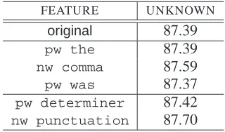
Table 1: Results for Probabilistic Context Features
FEATURE UNKNOWN OVERALL 5 buckets,pw the 87.20 96.97
5 buckets,nw comma 87.34 96.98
10 buckets,pw the 86.76 96.94
10 buckets,nw comma 87.15 96.95
10 buckets,pw was 87.34 96.96
Table 2: Results using binned features
To begin with, we chose a simple feature, that we can intuitively see should help discriminate be-tween classes. This feature is previous word (pw) the, that is, a real-valued feature describing the proportion of times in which we see the before the unknown word we are trying to find information on, compared to how many times we see the word at all. The idea of this feature is to tell when the unknown word we are looking at is a noun. This is because the determiner-noun pair is very common, and the is the most frequent determiner.
More potential features were identified by look-ing at the most common errors made by the tagger. We found that the most difficult distinction to make is between adjectives and common nouns. It is obvi-ous that a feature with a better chance of increasing performance would solve the most common errors, and from this analysis it should therefore differenti-ate chiefly between nouns and adjectives. The fea-ture we found that satisfies this property, is next word (nw) comma, that is, the proportion of times that the word we are focusing on is followed by a comma. Adjectives are only very infrequently fol-lowed by a comma, while nouns are in such a posi-tion quite often.
Another feature that was also tried, again in an attempt to discriminate between the most problem-atic cases, waspw was. This feature came from the idea that adjectives will often follow the word was, but nouns will not. The results from using each of these three features is shown in Table 1.
five bins (divided as: 0, 0–1/3, 1/3–2/3, 2/3–1 and 1), and also ten equally spaced bins (0–0.1, 0.1–0.2, etc). As can be seen in Table 2, representing the information in this way actually causes a decrease in accuracy. This demonstrates that real-valued fea-tures can give an improvement that traditional bi-nary features are unable to reproduce.
5.1 Higher frequency contexts
One reason why thepw wasfeature may not be as effective as nw comma, is that the word was does not occur as frequently as commas do. Commas (and the) occur about five times as often as was. The less frequent a word is, the less reliable it will be as a feature in the way we are using it. The reason for this it that it reduces the statistical reliability of the counts we are using as input for the feature. The counts overall will be lower, which increases the chance that one unusual context will be seen more than it should be, compared to the context in which the word is normally seen. Also, there will be less chance of finding counts greater than zero. There may be many adjectives that are used a number of times in the unannotated corpus, but still do not oc-cur after the word was.
We next attempted to increase the counts ex-tracted from the unannotated corpus. Seeing as the idea of the pw the feature was to identify nouns seen in a determiner-noun pair, one can expand the feature to become:pw determiner. Although the probabilities for what tags will follow a determiner are actually very close to those for the word the, the number of determiners in the unannotated corpus is significantly larger than just the word the.
We can also apply this idea to ournw comma fea-ture, by expanding it into anw punctuation fea-ture. The results of experiments run with these new expanded features are also shown in Table 1. One can see that they were indeed more effective than the simpler features they replaced.
5.2 Contexts from the Penn Treebank
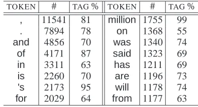
In order to find new features, we are looking for words that occur frequently and consistently have a certain tag before or after them. A list of tokens that meet these criteria can easily be found for each tag, by analysing the Penn Treebank. The results of this analysis are shown in Table 3.
This table shows the most frequent tokens follow-ing nouns, and the percentage of the time that they follow a noun. The first entry, which contains a fea-ture we have already found to be useful, shows us that this analysis could give us more effective fea-tures. Some words however, million for example, are overly optimistic due to source of this data. The
TOKEN # TAG% TOKEN # TAG%
, 11541 81 million 1755 99
. 7894 78 on 1368 55
and 4856 70 was 1340 74
of 4171 87 said 1323 69
in 3311 63 has 1211 69
is 2260 70 are 1196 73
’s 2173 95 will 1178 74
for 2029 64 from 1177 63
Table 3: Most frequent tokens that follow nouns
TOKEN # TAG% TOKEN # TAG%
than 1089 54 venture 82 52
quarter 717 75 ones 61 77
week 433 52 transactions 59 51
income 392 71 term 59 55
period 240 67 factors 52 63
estate 213 93 spring 50 52
German 99 62 subordinated 48 62
thing 91 58 ventures 42 67
Table 4: Most frequent tokens that follow adjectives
FEATURE UNKNOWN
original 87.39
nw of 87.42
nw for 87.50
nw preposition 87.56
nw to be verbs 87.48
nw modals 87.42
nw and 87.42
pw possessive pronouns 87.42
pw adjectives 87.45
pw adverbs 87.42
Table 5: Results using analysis of the Treebank
Wall Street Journal will clearly contain many such words whose frequencies are not representative of what they should be in more general text.
We can compare these words to the most com-mon words that follow adjectives, shown in Table 4. The obvious differences visible here mean that the features we apply from this analysis should discrim-inate between nouns and adjectives well. Using this same technique for different classes, looking at pre-vious word and next, we are able to find a number of features, each of which supplies a minor increase in performance. These are shown in Table 5.
6 Probabilistic lowercase features
cat-1ST WORD 2FEATURES UNKNOWN OVERALL
No No 87.83 97.01
No Yes 88.52 97.05
Yes No 87.86 97.01
Yes Yes 88.49 97.04
Table 6: Lower case frequency feature results
egories. One common problem is trying to deter-mine whether a word is a proper noun or a common noun. This becomes particularly difficult when the best way of telling between these two classes: look-ing at capitalisation of the first letter, is not infor-mative. This can be the case when the word is the first in the sentence or where the whole sentence is in upper case. To solve this problem, we can use the information from an unannotated corpus. If we see a unknown word and it is capitalised, then we can check the unannotated corpus for it, seeing whether it ever occurs uncapitalised. If it does, then there is a good chance that it is not a proper noun at all, but has been capitalised in this case for another reason. We will represent this information in the model using a real-valued feature. It will be the proportion of times in which the word occurs in the unanno-tated corpus in lower case, compared to the number of times it occurs at all.
We performed experiments firstly with the lower case frequency of all words, and then using only in-stances of a word that weren’t beginning a sentence. This is because a word beginning a sentence is al-ways capitalised in English, whether it is a proper noun or not, which is precisely the bias we were try-ing to avoid. We also tried ustry-ing two features, with one active for the first word in a sentence, while the other was active for all other words. This is because it is words that are first in the sentence that we are specifically trying to correct errors with. With only one feature, it would not get a strong enough weight, since the information it is giving on words that are not first in the sentence is not very useful. Having two features however, frees them both to make bet-ter decisions more specifically on the incorrect cases we are trying to fix.
As can be seen from the results in Table 6, the increase in performance was significantly more than any that had been attained previously.
7 Probabilistic plural features
Next we attempt to solve the third most common error that the model makes: incorrectly tagging sin-gular proper nouns as plural proper nouns. The idea we can use to distinguish between them, is that if we find the unknown word in our unannotated corpus
with -s on the end, then we can assume it is plural in this case, and that it is singular where we are trying to tag it. Although not all plurals are created by the
-s ending, it is the case in the vast majority of times,
and so we believe it will be effective enough. Im-plementing this as a feature, we attained an increase in unknown word accuracy to 87.61%.
This increase is greater than what most other fea-tures have achieved. It is interesting to note that most of the errors of tagging singular proper nouns as plural proper nouns consist of words such as
American Airlines. Here, Airlines should be tagged
as singular, but it still has the -s ending, so we would not expect our feature to help at all. An analysis of the errors fixed by this new feature shows that it ac-tually helped to distinguish between nouns and ad-jectives. This can be understood, as if the unknown word in the test corpus appears with an -s on the end in our unannotated corpus, it suggests that it is a noun in both cases. Adjectives are not affected by the addition of an -s in any normal grammatical way, and so we would expect the chance of seeing such a construction to be much less.
8 Using multiple real-valued features
All the experiments we have described so far have included only one feature at a time (with the excep-tion of lower case frequency, which uses two). Of course, we can use all of them at once, collecting information from all of them.
We also tried combining the features in a differ-ent way. Rather than having one feature for each piece of information we are giving the model, we could add up the counts used for each feature, cre-ating one feature with larger, and hopefully more reliable counts than any of those that it is made up of. We then have one feature in the model for all these pieces of information. The value for this fea-ture could exceed one, and so we experimented with limiting the value at one, or simply allowing it to take on whatever value it would.
The features that we used included all those that had individually given a positive result. Thelower case frequency feature was also used, as was
word exists with -s, although these two were not summed with the other features, as they are of a different nature. The results achieved, are shown in Table 7.
9 Analysis
COMBINATION METHOD UNKNOWN OVERALL
original 87.39 96.99
all positive 88.82 97.05
all positive, summed 88.85 97.05
all positive, summed with a limit of 1 88.82 97.05
Table 7: Accuracies from combining all positive features
UNKNOWN ORIGINAL nw punctuation lower case freq. ALL POSITIVE WORD% UNK. ALL UNK. ALL UNK. ALL UNK. ALL 1 2.81 87.39 96.99 87.70 97.00 88.52 97.05 88.82 97.05 1/2 4.15 86.49 96.61 86.63 96.62 87.89 96.68 88.35 96.71 1/4 6.08 86.22 96.28 86.65 96.31 87.42 96.37 87.97 96.44 1/8 8.56 85.67 95.53 85.94 95.56 86.60 95.64 87.34 95.81 1/16 11.99 84.90 94.73 84.95 94.76 86.02 94.91 86.65 95.18
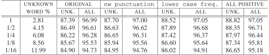
Table 8: Results with reduced training data
able to test our new features on a corpus from a dif-ferent domain, since this is the kind of application where our features should perform the best. Unfor-tunately, there is no such corpus that is substantial enough for our purposes, which has the annotations that we would need to measure accuracy. As a result of this limitation, we will instead rely on a different technique to simulate tagging a piece of text with more unknown words.
9.1 Reducing the training dataset
We can reduce the amount of data used for train-ing, thereby increasing the proportion of unknown words. This will also mean the tagger has less idea of the way words are used in general, which is an-other effect that we would like to mimic. Although the words themselves will still be drawn from the same financial newspaper text, and therefore exhibit all the same grammatical tendencies, we can still get an idea of how effective our new features are in a situation they are actually well-suited for.
Experiments were performed with a half, a quar-ter, an eighth, and a sixteenth of the training data, with the results shown in Table 8. The precentage of unknown words grows exponentially as the size of the training data decreases. This means that as we move to smaller training sets, unknown words rapidly become a more significant problem.
As would be expected, using a smaller training set reduces the performance of the tagger quite con-siderably. However, the improvements gained from using the new features remain consistent.
Even more encouraging is the way the overall re-sults begin to improve. This stems from the fact that the unknown words are beginning to take up a more
significant proportion of the text. This demonstrates that our new features are indeed able to raise accu-racy in the area that they were designed to.
9.2 Cross Validation Experiments
We have also carried out an experiment using 10-fold cross validation. We split the entire Penn Tree-bank, putting every nth line into the nth fold. This configuration results in a similar percentage of un-known words as in previous experiments. The accu-racy for the original system are 97.12% overall and 89.13% on unknown words only. Using the sum-mation of all positive features, as well as the best
lower case frequency feature and the word exists with -s feature, we achieved 97.15% overall and 90.17% on unknown words. This is an accuracy increase of 1.04% on unknown words which confirms the statistical validity of the results we have attained previously.
10 Named Entity Recognition
We have also experimented with the task of Named Entity Recognition (NER) in almost the same man-ner as we have described for POS tagging. We will use contextual information from the same unanno-tated corpus, in order to better classify a certain sub-set of the test corpus. In this case, the named entities themselves, while for POS tagging we looked at the unknown words.
FEATURE PRECISION RECALL F-SCORE
original 86.55 86.78 86.66
nw preposition 86.64 86.87 86.75
pw preposition 86.69 86.69 86.69
pw locative preposition 86.79 86.87 86.83
pw said 86.64 86.87 86.75
pw speech marks 86.55 86.78 86.66
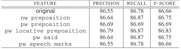
Table 9:NERresults
in our POS tagging corpus. We performed an anal-ysis on this dataset, as we did for POS tagging, at-tempting to find words that could be used as suitable features. Some of those we found are shown in Ta-ble 9, as well as the increases in accuracy that come from using them. We also experimented with the features that performed well in POS tagging, and found that they did not work as well at this task.
We can see that use of the pw locative preposition feature provided the greatest in-crease in accuracy. This feature was specifically used to identify locations, as they are often pre-ceeded by words such as to, from, and in.
11 Discussion
What we have seen is thatnw punctuation per-forms the best out of the next word/previous word features, while word exists with -s is also useful, outperforming many of them. Lower case frequency is quite easily our best feature, as it cor-rects so many of the errors that occur with proper nouns. Using all our features together, we find that even the minor increases gained by some of the indi-vidual features can be translated to an overall gain.
Our second technique for combining multiple features, that of summing the feature values to-gether, has also been shown to give satisfactory re-sults. The effect of having larger, more reliable counts was apparently able to compensate for the conflation of some information upon amalgamation. All of our experiments and analysis have sug-gested two measurable quantities to identify a good feature. The first of these is to discriminate well be-tween two possible classes, especially those classes that exhibit a high level of confusion. Here,pw the
was not able to differentiate between noun and ad-jectives, whilenw commawas. The second measure is the frequency of the word we are basing our fea-ture upon, with more common words being better. For example, the pw wasfeature did not perform nearly as well asnw comma.
We used these ideas to find a number of produc-tive features. Problem cases with the existing tag-ger gave us particular areas for improvement, such
as the noun-adjective discrepancies. Further anal-ysis of common word/tag combinations in the an-notated corpus also gave us a number of worth-while features. However, it should be noted that we did require the annotations for this analysis, as well as to implement some other features, such as
pw unambiguous adjective. Seeing as a large annotated corpus, the Penn Treebank, is only avail-able for English, we would have a problem shifting our focus toPOStagging in another language.
One thing that we have achieved is the imple-mentation and use of real-valued features. They were able to outperform traditional MaxEnt fea-tures, finding an increase in accuracy where dis-cretized features could not. In particular, one would not be able to represent the features that we are using in the Maximum Entropy model, and still gain an increase in performance, without using real-valued features. One can easily see more possibil-ities for their use, as they are a much more natural way of representing many attributes in a machine learner.
12 Future Work
The real-valued features we have described are specifically designed at better classify unknown words. We would therefore like to test our approach in a domain where unknown words are more preva-lent. We would also like to try using a different, larger unannotated corpus, even when working with the Penn Treebank test corpus.
Using a larger raw corpus would mean that more of the unknown words could be found, and there-fore that there would be a chance for correcting er-rors with these unknown words. Also, the unknown words that are already present in the Aquaint cor-pus we used would have bigger counts in a larger corpus. We would therefore be able to get more re-liable information about them, and a better idea of how they are used.
mat-ter what context it is in. That one instance will make the feature value either 0 or 1, the two most extreme values, which may be tremendously misrepresenta-tive of what the true value should be.
There are many smoothing methods that can help with this problem. The Good-Turing estimation is one approach which calculates estimated values us-ing the observed counts for the next most frequent word (Good, 1953). It is extremely effective for words with low counts, and would therefore be able to solve this problem quite well.
Another smoothing issue comes from the Gaus-sian prior that is used within the Maximum Entropy training code. This prior has the effect of keeping the weights within a normal distribution, slightly re-laxing the constraints upon the model. It has the effect of not allowing any single weight to get too large, which could mean many tagging decisions were made on a single, possibly unreliable, feature. However, the algorithm does not take into account the introduction of real-valued features, and there-fore the possibility of non-binary feature values. As a result of this, some real-valued features may be prevented from having as large a weight as they should, and thus having reduced impact. An investi-gation into what effects this problem has, as well as changing the implementation to calculate the update values more correctly, would be beneficial.
13 Conclusion
We aimed to use the information in an unannotated corpus — in particular, the contexts surrounding un-known words — in order to increase performance on POS tagging unknown words. Although a num-ber of techniques have been applied to this problem in the past, none attempted to draw upon the infor-mation that could be found in a larger amount of raw text. The new feature types we have demon-strated are quite different to those previously used, and we have shown the increase in performance that they can give. The advantage of this method is that it can derive contextual information from any unan-notated corpus, and so it is easily portable to another domain.
In particular, the use of real-valued features re-sulted in a much larger improvement than binary or discretized features would have given us. Maxi-mum Entropy features in the past have always been limited in this respect, and seeing the results we attained, one cannot doubt the benefits that real-valued features can bring. The increased flexibility they give us, and their ability to capture relation-ships between values, make them extremely advan-tageous. One can see that the kind of information
we were trying to represent was a good example case for their usage, but there are many other fea-tures that would also be intrinsically suited to them. The increase of 1.46% on tagging accuracy for unknown words raises the result to a state-of-the-art level, which will translate to benefits when perform-ing other NLPtasks based onPOS tagging informa-tion. The smaller increase forNERshows that these methods are also feasible for other tagging tasks, and demonstrates once again, the usefulness of real-valued features.
Acknowledgements
We would like to thank members of the Language Technology Research Group and the anonymous re-viewers for their helpful feedback. This work has been supported by the Australian Research Council under Discovery Project DP0453131.
References
A. Berger, S. Della Pietra, and V. Della Pietra. 1996. A maximum entropy approach to natural language pro-cessing. Computational Linguistics, 22(1).
E. Brill. 1994. Some advances in rule based part-of-speech tagging. In Proceedings of the Twelfth
Na-tional Conference on Artificial Intelligence, pages 722
– 727, Seattle, WA.
S. Chen and R. Rosenfeld. 1999. A gaussian prior for smoothing maximum entropy models. Technical re-port, Carnegie Mellon University.
J. R. Curran and S. Clark. 2003. GIS and smoothing for maximum entropy taggers. In Proceedings of the
11th Conference of the European Chapter of the Asso-ciation for Computational Linguistics, pages 91 – 98,
Budapest, Hungary.
DARPA. 1998. Proceedings of the seventh message un-derstanding conference (MUC-7). Fairfax, Virginia. Morgan Kaufmann Publishers, Inc.
J.N. Darroch and D. Ratcliff. 1972. Generalised iterative scaling for log-linear models. Annals of Mathematical
Statistics, 43:1470 – 1480.
D. Graff. 2002. The AQUAINT corpus of English news text. Technical Report LDC2002T31, Linguistic Data Consortium, Philadelphia.
M. P. Marcus, B. Santorini, and M. A. Marcinkiewicz. 1993. Building a large annotated corpus of En-glish: The Penn Treebank. Computational
Linguis-tics, 19(2):313 – 330.
A. Mikheev. 1997. Automatic rule induction for un-known word guessing. Computational Linguistics, 23(3):405 – 423.
A. Ratnaparkhi. 1996. A maximum entropy part-of-speech tagger. In Proceedings of the EMNLP. R. Weischedel, M. Meteer, R. Schwartz, L. Ramshaw,
and J.Palmucci. 1993. Coping with ambiguity and unknown words through probabilistic models.