R E S E A R C H
Open Access
Optimal interference range for minimum
Bayes risk in binomial and Poisson wireless
networks
Min Ouyang, Wenxiao Shi
*, Ruidong Zhang and Wei Liu
Abstract
Interference is the main performance-limiting factor in most wireless networks. Protocol interference model is extensively used in the design of wireless networks. However, the setting of interference range, a crucial part of the protocol interference model, is rather heuristic and remains an open problem. In this paper, we use the stochastic geometry and the direct approach to obtain the associated feasibility distributions. After that, we use the binary hypothesis testing to achieve the Bayes risk under binomial point process (BPP) and Poisson point process (PPP), respectively. According to the first derivative of the Bayes risk, we provide the equation to achieve the optimal interference range for minimum Bayes risk. We extend the method proposed by Wildman et al. to a more general situation. Furthermore, we show that for infinite PPP, those two methods converge to the same results. Several numerical results for wireless networks under BPP, finite PPP, and infinite PPP are given. Simulation results show that in the finite wireless network, the BPP method performs better than the PPP method.
Keywords: Bayes risk, Binary hypothesis testing, Interference range, Stochastic geometry, Wireless networks
1 Introduction
Interference range is a crucial part of the protocol inter-ference model. Under the protocol interinter-ference model, the transmission between the reference receiver and the ref-erence transmitter is successfully received, when there is no interference transmitter within the interference range of the reference receiver [1]. In the last two decades, inter-ference range is widely used in wireless networks, such as ad hoc networks [2–5], wireless mesh networks [6–10], sensor networks [11, 12], cellular networks [13, 14], and WiMAX networks [15]. The setting of interference range has a large effect on the performance of wireless networks [10, 11, 16, 17]. In wireless networks based on the IEEE 802.11 standard, interference range is usu-ally set to be twice as large as the transmission range [7,8,18,19]. In CSMA-based wireless networks, the inter-ference range is set equal to the carrier sensing range [4,6,9,20]. Several works [2,4,21–23] set the interference range by restricting the signal-to-interference-and-noise
*Correspondence:[email protected]
1College of Communication Engineering, Jilin University, Nanhu Road, 130012 Changchun, China
ratio (SINR) to a threshold. In their works, only one inter-ference transmitter is considered when calculating the SINR. The interference ranges in the mentioned literature are set without fully considering the effect of the net-works. However, the optimal interference range may be a function of network parameters, and the casual setting of the interference range will depress the performance of wireless networks. The setting of the interference range is rather heuristic and remains an open problem [24].
Several works have further studied the setting of the interference range. Hasan and Andrews [25] study the optimal interference range (guard zone) to maximize transmission capacity in CDMA-based wireless ad hoc networks. Iyer et al. [26] study the minimum interference range under the additive interference model, the cap-ture threshold model, and the interference range model, respectively. Zhou et al. [15] deduce the probability den-sity of the ratio between the interference range and the one-hop distance. The randomness of the ratio is due to the random thermal noise. Besides, they only consider one interference transmitter. Shi et al. [24] discuss the bounds for the maximum interference range. They deduce the lower bound of the maximum interference range with
the maximum transmission range, and the upper bound with the maximum range that a band can be reused. Their work gives the span of maximum interference range. However, the exact value of the interference range remains unknown.
Zhang et al. [27] propose the physical-ratio-K (PRK) interference model as a reliability-oriented instantiation of the protocol model. Furthermore, they study the effect of K on the reliability and throughput. Hasan and Ali [28] present the optimal interference range (guard zone) expression that maximizes the density of successful trans-missions under an outage constraint. Wildman and Weber [29] study the optimal interference range to minimize the Bayes risk of the protocol interference model in wireless Poisson networks. In [30], they also investigate the inter-ference range to maximize the correlation of the physical interference model and protocol interference model in Poisson networks. The authors use the binary hypothe-sis testing to achieve the interference range for minimum Bayes risk. However, their works are only suitable for Poisson networks. The Poisson point process has two defi-ciencies when modeling finite networks. The first one is no consideration of the network boundary. The second one is the allowance of unbounded nodes in a finite area. The optimal interference range for finite network needs further study.
In this paper, our main contribution is proposing a method of setting the optimal interference range which is applicable for a more general situation. We employ the binary hypothesis testing framework to outline the relationship between the physical and protocol interfer-ence model. The optimal interferinterfer-ence range is configured to minimize the Bayes risk of the protocol interference model.
The first contribution of this paper is proposing a method to achieve the optimal interference range for binomial wireless networks. We adopt the direct approach to obtain the associated feasibility distributions for wire-less networks under BPP. Furthermore, we calculate Bayes risk with those distributions and deduce the optimal inter-ference range to minimize the Bayes risk.
Next, we derive the optimal interference range for finite and infinite Poisson wireless networks. Furthermore, we demonstrate that the optimal interference range found by Wildman et al. [30] is the special case of the infinite PPP.
Finally, we present several numerical results of Bayes risks, receiver operating characteristic (ROC), and area under curve (AUC) under BPP, finite PPP, and infinite PPP. Our results reveal that the BPP method and the finite PPP method achieve smaller optimal interference range than the infinite PPP method. In the finite wireless network, the BPP method performs better than the PPP methods.
The rest of this paper is organized as follows. In Section 2, we introduce the wireless network model,
including the propagation model, physical interference model, and protocol interference model. In Section3, we introduce the binary hypothesis testing and Bayes risk. In Section 4, we provide the feasibility distributions under binomial wireless networks and Poisson wireless net-works, respectively. In Section5, we deduce the Bayes risk and optimal interference range. In Section6, we give some numerical results for BPP and PPP. Section7 concludes this paper. Finally, for clarity, long proofs are presented in theAppendix.
2 Network model
We consider a network, in a two-dimensional region A, with a reference receiverRX0, a reference transmitterTX0, andMinterference transmittersTX1,· · ·,TXM. Assume
that all interference transmitters are active and consist of a point process in a snapshot. In this paper, we concen-trate on analyzing the performance (the Bayes risks) of the networks at a snapshot with stochastic geometry tool. For the analyzing of the long-term metrics, queuing theory should also be incorporated [31]. Without a loss of gener-ality, due to the stationarity of the point process, we may take the reference receiver to be at the origin. The distance is normalized by the distance fromTX0toRX0, denoted byd0=1. Letdidenote the distance fromTXitoRX0. The area of the network region is denoted by|A|. As the power allocation is not considered in this paper, we assume that all transmitter’s powerPifor alli∈ {0,· · ·,M}is the same.
2.1 Propagation model
Our signal propagation model considers the path loss with Rayleigh fading. The signal received by RX0 from TXi,
denoted byPRi, is
PRi=Pihid−i α (1)
wherehiis the i.i.d. unit-mean exponential shadowing
fac-tor for alli∈ {0,· · ·,M},α >2 is the path loss exponent. The value of α is typically between 2 and 8 as in [32] and [33].
2.2 Physical interference model
Under physical interference model, transmission from TX0is successfully received byRX0if the SINR is no less than a defined SINR thresholdβ, which can be expressed as follows:
SINR= h0
SNR−1+M
i=1
hid−i α
≥β (2)
and the SNR−1 is achieved by dividing the transmitter powerP0with the average noise.
Let random variablesH = 1{SINR≥β}represent the physical model feasibility, denoted byH1, of the transmis-sion fromTX0toRX0. The indicator1Ahas the value 1 for
all elements ofAand the value of 0 for all elements not in A. The physical model failure is denoted byH0.
2.3 Protocol interference model
Under protocol interference model, a transmission from TX0toRX0is successful, if there are no interference trans-mitters within the interference range ofRX0, denoted by
RI. Let random variablesD = 1{di≥RI,∀i=0}
repre-sent the protocol model feasibility, denoted byD1, of the transmission fromTX0toRX0. The protocol model failure is denoted byD0.
3 Binary hypothesis testing and Bayes risk
In wireless networks, the physical interference model is considered as a more realistic description of the effects of interference [35]. Appropriate setting of the interference range of the protocol interference model can maximize the similarity between the two models. The appropri-ate setting here means to set the interference range to be the optimal interference range which maximizes the similarity. In this paper, we employ the binary hypothe-sis testing framework in [36] to describe the relationship between the two models. The minimum Bayes risk maps the maximum similarity. The optimal interference range to maximize the similarity between the two models is equivalent to minimize the Bayes risk.
In the binary hypothesis testing, the two hypotheses (null hypothesis H0and alternate hypothesis H1) repre-sent the possible outcomes (failure and success) under the physical interference model. The two decisions (D0 andD1) represent the possible observations (failure and success) under the protocol interference model. For this binary hypothesis testing problem, four possible cases can occur:
(1) DecideD0whenH0is true. (2) DecideD0whenH1is true. (3) DecideD1whenH0is true. (4) DecideD1whenH1is true.
In order to use the Bayes’ criterion, we assume that a cost is assigned to the possible decisions. We can define Cij
i,j=0, 1as the cost associated with the decisionDi,
when hypothesisHjis true. In particular, the costs for this
binary hypothesis test problem areC00to case (1),C01to case (2),C10 to case (3), andC11to case (4). The goal in our Bayes’ criterion is to determine the optimal interfer-ence range to minimize the average costE[C], also known as Bayes riskrin [29]. DenotePDiHj
as the joint prob-ability that we decideDiwhen the hypothesisHj is true.
The Bayes risk is
The costCijmay be chosen to be particular network
per-formances. In this paper, we use the uniform cost model (C00 = C11 = 0 andC01 = C10 = 1) for simplicity. This assumption is reasonable, as there is no cost of similarity when the two models make the same decision, as in [29] and [30]. From Bayes’ rule, the Bayes risk can be expressed as follows:
r = P(D0,H1)+P(D1,H0)
= P(H1)+P(D1)−2P(H1|D1)P(D1) (4) where P(H1) and P(D1) are the probabilities of phys-ical and protocol feasibility distribution, respectively. P(H1|D1) is the conditional feasibility distribution of physical model given successfully received of the protocol model. Those feasibility distributions will be deduced in the following section.
4 Feasibility distributions
Based on the network model and according to the stochas-tic geometry, we provide the feasibility distributions of binomial and Poisson wireless networks.
4.1 Binomial wireless networks
Assume that M interference transmitters are indepen-dently and uniformly distributed over A. A is a circle center at the origin with radius of R. Thus, the inter-ference transmitters are drawn from a BPP of density
λ=MπR2. We denote the BPP byM. According to
the coverage probability of [34] and the standard results in stochastic geometry [37], following three distributions can be obtained.
Lemma 1 The feasibility distribution of the physical model under BPP is and2F1is the Gauss hypergeometric function, 2F1([a,b] ;c,x)
ProofThis result follows from [34], by setting the exclu-sion zone radius (the area of no active interference trans-mitters) rin to be zero and the transmitting probability
to setrin to be zero. For the simplicity of derivation, we
set the transmitting probability to be one, as in [29] and [30]. When considering transmitting probability, the fea-sibility distribution can also be calculated. More complex and challenging cases with spatio-temporal traffic, where pis decided by a stochastic process, can be investigated by combining stochastic geometry and queuing theory as in [38].
Lemma 2 The feasibility distribution of the protocol model under BPP is
PBPP(D1)=
1−R 2
I
R2 M
(6)
ProofAccording to [37], for a binomial point process withMpoints in a compact setA, the void probabilities of a point process are the probabilities of there being no point of the process in given test setsB:
P(N(B)=0)= (vd(A)−vd(B))
M
vd(A)M
(7)
where N(B) is the number of point in B, vd(B) is the
volume ofB.
The feasibility distribution of the protocol model under BPP, denoted byPBPP(D1), is the probability of there being no point of interference transmitter in the interference range of the reference receiver. The interference range in this paper is the circle centered at the reference receiver with radiusRI. Substitute the interference range forB,πR2I
forvd(B), andπR2forv
d(A)achieves Lemma2.
Lemma 3The conditional feasibility distribution of physical model given successfully received of protocol model under BPP is
PBPP(H1|D1)=e−ζ
1+ (R)− (RI) R2
M
(8)
ProofSimilar to the proof of Lemma1, this is achieved by setting the exclusion zone radiusrin to beRI and the
transmitting probability p to be one. Here, we set the exclusion zone radius to be RI, means there being no
interference transmitter in the interference range.
Other distributions, derived fromHandD, are express-ible in terms ofPBPP(H1|D1),PBPP(H1), andPBPP(D1).
4.2 Poisson wireless networks
Assume that the interference transmitters are drawn from a PPP, denoted by , with densityλ overA. Ais a cir-cle center at the origin with a radius ofR. The number of interference transmittersMwithin regionAis Poisson with mean E[M] = λπR2. The feasibility distributions
can be obtained by taking the expectation of the three distributions in BPP with respect toM.
Lemma 4 The feasibility distribution of the physical model under PPP is
PPPP(H1)=exp{−ζ +λπ (R)} (9)
Proof Similar to the proof of Lemma1, this result fol-lows from [34], by setting the exclusion zone radiusrinto
be zero and the transmitting probabilitypto be one.
Lemma 5 The feasibility distribution of the protocol model under PPP is
PPPP(D1)=exp
−λπR2I (10) Proof From [37] we know, in a homogeneous Poisson point process with density λ, the void probabilities of a point process are the probabilities of there being no point of the process in given test setsB:
P(N(B)=0)=exp{−λvd(B)} (11)
where N(B) is the number of point in B, vd(B) is the
volume ofB.
The feasibility distribution of the protocol model under PPP, denoted byPPPP(D1), is the probability of there being no point of interference transmitter in the interference range of the reference receiver. The interference range in this paper is the circle centered at the reference receiver with radiusRI. Substitute the interference range forB, and
πR2I forvd(B)achieves Lemma5.
Lemma 6The conditional feasibility distribution of physical model given successfully reception of protocol model under PPP is
PPPP(H1|D1) = exp{−ζ +πλ (R)
− πλ (RI)} (12)
Proof Similar to the proof of Lemma3, this result fol-lows from [34], by setting the exclusion zone radiusrinto
beRIand the transmitting probabilitypto be one.
Other distributions, derived fromHandD, are express-ible in terms ofPPPP(H1|D1),PPPP(H1), andPPPP(D1).
5 Optimal interference range
networks. Furthermore, the Bayes risk and optimal inter-ference range in infinite Poisson wireless networks can be found by taking the limit of those in the finite Poisson wireless networks asR→ ∞.
5.1 Binomial wireless networks
Proposition 1The Bayes risk in binomial wireless networks, denoted by rBPP, under the uniform cost model is
rBPP = PBPP(H1)+PBPP(D1)
− 2PBPP(H1|D1)PBPP(D1)
= e−ζ
1+ (R) R2
M
+
1−R 2
I
R2 M
− 2e−ζ
1+ (R)− (RI) R2
M
×
1− R 2
I
R2 M
(13)
ProofThe result is immediate from (4) and substi-tuting feasibility distribution expression from (5), (6), and (8).
Theorem 1(Optimal interference range for minimum Bayes risk)Under the uniform cost model, the optimal interference range for minimum Bayes risk in binomial wireless networks always exists. Whenζ ≥log 2, the opti-mal interference range is R. This can hardly be set as inter-ference range, as only the reinter-ference transmitter is allowed to transmit. Whenζ < log 2, the optimal interference range is the unique solution to
eζ1+( (R)− (RI))R2−M=
2− 2βR
R2−R2I RI
β+RαI R2+ (R)− (R
I)
(14)
ProofThe proof is in AppendixA
5.2 Finite poisson wireless networks
Proposition 2The Bayes risk under finite PPP, denoted by rPPP, under the uniform cost model is
rPPP = PPPP(H1)+PPPP(D1)
− 2PPPP(H1|D1)PPPP(D1)
= exp{−ζ+λπ (R)} +exp−λπR2I − 2 exp{−ζ+λπ (R)
− λπ (RI)+R2I
(15)
ProofSimilar to Proposition1by substituting feasibility distribution expression from (9), (10), and (12).
Theorem 2(Optimal interference range for minimum Bayes risk)Under the uniform cost model, the optimal interference range for minimum Bayes risk under finite PPP is the unique solution to
β+RαI
2RαI =exp{−ζ+λπ (R)−λπ (RI)} (16) The solution exists if and only if
ζ <log2Rα/β+Rα (17)
ProofThe proof is in AppendixB.
5.3 Infinite poisson wireless networks
For the PPP on the entire plan, the corresponding results can be obtained from the PPP over a finite regionAby taking the limit as R → ∞. The results are as follows. The feasibility distributions of infinite PPP are similar to those of finite PPP by replacing (R) to lim
R→∞ (R) =
−2πβ2/αcsc(2π/α)/αcsc(2π/α) /α. The Bayes risk is
rinfPPP=exp
−ζ−2λπ2β2/αcsc(2π/α)/αcsc(2π/α) /α
+exp
−λπR2I
−2 exp{−ζ −2λπ2β2/αcsc(2π/α)α − λπ (RI)+R2I
(18)
Corollary 1(Optimal interference range for minimum Bayes risk)Under the uniform cost model, the optimal interference range for minimum Bayes risk under infinite PPP is the unique solution to
β+RαI 2RαI = exp
−ζ−2λπ2β2/αcsc(2π/α)/α
− λπ (RI)} (19)
The solution exists if and only if
ζ <log 2 (20)
ProofThis result follows from Theorem2by taking the limit asR→ ∞.
Corollary 2 For two dimension networks, when the reference transmitter is at unit distance from the receiver and uniform cost model is adopted, the Bayes risk and the optimal interference range under infinite PPP are the same with those in[30].
6 Numerical results
In our simulation, we use the similar environment param-eters of [30]. Notice that distance is normalized to the distance from TX0 to RX0, and the transmitter density is one hundred times of that in [30]. Numerical results for Bayes risk, optimal interference range, receiver oper-ating characteristic (ROC), and area under curve (AUC) for both BPP and PPP are shown as follows. The pro-posed methods can be adopted to achieve the interference range for wireless networks. We utilize the ROC and AUC to evaluate the performance of each method. The ROC is used to show the tradeoff between type I (false rejec-tionPI =P(D1|H0)) and type II (false acceptancePII =
P(D0|H1) ) error rates. The AUC is the area under the ROC curve and is a useful numerical value to evaluate the performance of the proposed method.
6.1 Bayes risks and first derivatives
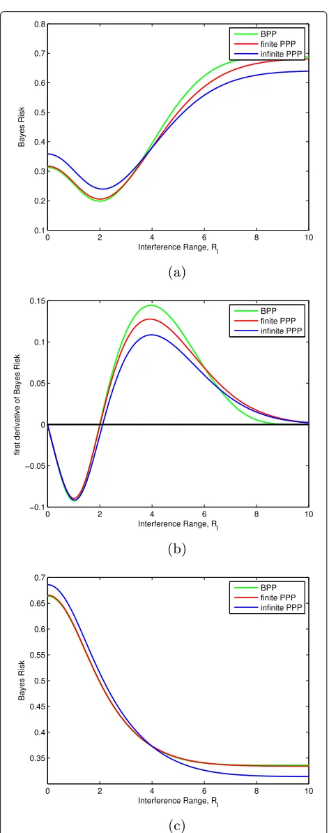
The Bayes risks and the first derivatives under BPP, finite PPP, and infinite PPP are shown in Fig1. In order to show the difference of the three point processes, we set the area to be a disk of radiusR=10. When the area is sufficiently large, the results of BPP and finite PPP converge to those of infinite PPP. The density of interference transmitter is
λ=2×10⁻². The path loss exponent isα=3. The SINR threshold isβ = 5. We first investigate the case without noise, where the power of background noise is set to be 0, and the SNR is infinite, i.e., SNR= +∞.
Figure 1a shows the Bayes risks decrease firstly then increase with the increment of the interference range. The minimum Bayes risks are achieved at the optimal interference range. From the numerical results, we know that there is a unique optimal interference range which can minimize the Bayes risk for BPP, finite PPP, and infi-nite PPP, respectively. For BPP, the optimal interference range isRBPPI =2.00. For finite PPP, the optimal interfer-ence range isRPPPI = 2.02. For infinite BPP, the optimal interference range is Rinf PPPI = 2.11. This indicates the BPP has the smallest optimal range, which allows more transmitters to be active simultaneously. Besides, with small interference range, the Bayes risk of BPP is almost the same as the Bayes risk of finite PPP, and obviously smaller than that of infinite PPP. This means, for finite net-works with small interference range, using the infinite PPP method will overestimate the Bayes risk.
As shown in Fig 1b, with the growth of interference range, the first derivatives turn from negative to posi-tive. For 0 < RI < 10, there is a unique zero point,
which acts as the optimal interference range, for the BPP, finite PPP, and infinite PPP, respectively. It can be found that the first derivative of the BPP is the first to reach the zero point, and follows the first derivative of the finite PPP, and the last is the first derivative of the infinite PPP.
When SNR is sufficiently largeSNR> log 2β , similar results can be achieved. For the case with large noise
SNR≤ log 2β , we set SNR=7 as an example in Fig1c. It is obvious that the Bayes risks are monotonously decreas-ing, and the optimal interference ranges for the mini-mum Bayes risks are at the maximini-mum network radiusR. This indicates that only the reference transmitter can be active, which is inefficiency for a practical network. Con-sequently, the Bayes methods cannot be directly applied to the network with heavy noise, and more effort should be taken in this aspect.
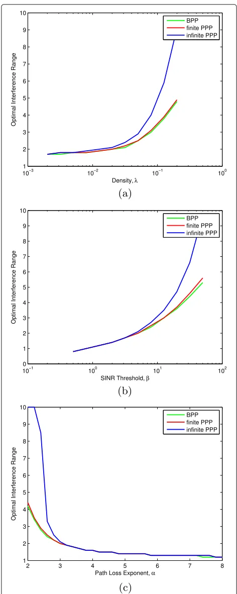
6.2 Parameters influence the optimal interference range Figure2shows the optimal interference range influenced by parameters(λ,β,α), under BPP, finite PPP, and infinite PPP. The area is a disk of radiusR = 10. The power of background noise is set to be 0, and the SNR is infinite, i.e., SNR= +∞.
Figure 2a shows the optimal interference ranges increase with the density λ growing from 2× 10⁻³ to 2× 10⁻¹. The settings of other parameters areα = 3 and β = 5. This is quite hard to understand. As the physical feasibility decreases withλ, in order to minimize the Bayes risks, the protocol feasibility must likewise be decreased by increasingRI orλ. Notice that, in order to
minimize the Bayes risks, only increasingλis not enough, and it must be additionally increased by expandingRI. It
is quite obvious that the optimal interference range of BPP and finite PPP are smaller than that of infinite PPP. As in infinite PPP, the network radius is infinite, which leads to more interference compared with BPP and finite PPP. In order to minimize the risk, a relatively larger interfer-ence range is needed for infinite PPP. Besides, the optimal interference range of BPP is slightly lower than that of finite PPP.
Figure 2b shows the optimal interference ranges increase with the SINR thresholdβ growing from 0.5 to 50. The settings of other parameters areλ=2×10⁻²and
α = 3. This is because the physical feasibility decreases with SINR thresholdβ, and the protocol model feasibil-ity must be decreased by increasingRI. Similar to Fig.2a,
the optimal interference range of BPP and finite PPP are smaller than that of infinite PPP, and the optimal inter-ference range of BPP is slightly lower than that of finite PPP.
Figure 2c shows the optimal interference ranges decrease with the path loss exponent α growing from 2 to 8. The settings of other parameters are λ = 2 × 10⁻² and β = 5. Bigger path loss exponent means higher power attenuation, which leads to lower interference and higher protocol feasibility. In order to minimize the Bayes risks, the protocol feasibility must likewise be increased by decreasing RI. Again,
the optimal interference range of BPP and finite PPP are smaller than that of infinite PPP, and the optimal interference range of BPP is slightly lower than that of finite PPP.
Those simulation results indicate the optimal interfer-ence range should be appropriately chosen according to the network parameters. The casual setting of the inter-ference range will raise the Bayes risk and depress the performance of wireless networks.
6.3 ROC and AUC compare
Figure3compares the ROC and AUC of BPP, finite PPP, and infinite PPP. The path loss exponent is α = 3. The SINR threshold is β =5 and SNR = +∞. Figure 3a shows the ROC curves travel from bottom-right to top-left, as the interference range RI grows. The network
Fig. 3ROC and AUC compare.aROC for BPP, finite PPP, and infinite PPP.bAUC for BPP, finite PPP, and infinite PPP
radius isR=10. The density of interference transmitter is
λ = 2×10⁻². The ROC of BPP is in the lowest place and close to the ROC of finite PPP. It is obvious that the ROC of both BPP and finite PPP is under that of infinite PPP, which means the BPP and finite PPP methods have a lower error rate than the infinite PPP method. That is to say, the BPP method and the finite PPP methods perform better in the finite networks. Figure3b shows the AUC of BPP, finite PPP, and infinite PPP vary with the different network radiuses. The network radiuses range from 10 to 200, and the density of interference transmitter is set to be
λ = 2×10⁻²,λ = 1×10⁻¹, andλ = 3×10⁻¹. From the simulation results, we know the AUC of BPP and finite PPP is smaller than the AUC of infinite PPP when the net-work radius is small. With a larger netnet-work radius, those AUCs are nearly the same. Those results indicate that the BPP method and the finite PPP method have better per-formance in small networks and have similar perper-formance to infinite PPP in large networks. Furthermore, whenλ= 1×10⁻¹andλ = 3×10⁻¹, there is an obvious advan-tage of the BPP method over the finite PPP method. That is to say, the BPP method performs better than the PPP methods in small networks with high node density. When
λ = 2 ×10⁻², the AUC of finite PPP and infinite PPP are nearly the same. This implies that the two PPP meth-ods have the same performance in wireless networks with large density.
7 Conclusion
In this paper, we provide methods to achieve the opti-mal interference range for minimum Bayes risk, under the assumptions of both binomial and Poisson wireless networks. For Poisson wireless networks, both finite and infinite networks are concerned. Following that, several numerical results are provided. Simulation results show that in the finite wireless network, the BPP method per-forms better than the PPP methods. The analytical and numerical results may assist in the more accurate and effective use of the protocol interference model.
In future work, it is of interest to relate the risk with what a user of networks may care, e.g., through-put, delay, and reliability. This may directly indicate the effect of interference range setting on the network per-formance. Additionally, networks with medium access control (MAC) protocol (e.g., ALOHA and CSMA), unsaturated traffic(e.g., spatio-temporal traffic), and more fading factors (e.g., Rician and Nakagami) need further studied.
Appendix Appendix A Proof of theorem 1
drBPP
In order to analyze the first derivative, the following two functions are defined.
The first derivative ofrBPPto interference rangeRIcan
be expressed as follows:
decreasing). The monotonicity of rBPP can be easily decided by analyzingf1−f2.
From (24), we know 1/f1 is monotonously increasing, andf1is monotonously decreasing. The limiting values are
lim
Forf2, the first derivative is
f2 = β+RαI R2+ (R)− (RI)−2
From (25), we knowf2is monotonously increasing, and the limiting values are lim
RI→0
In summary, f1 is decreasing from eζ
It is clear thatf1andf2have a unique intersection, which minimizes the Bayes risk, if and only if eζ < 2 , i.e.,
ζ < log 2. That is to say, when ζ < log 2, the opti-mal interference range is achieved at f1 = f2. Denote the pointf1 = f2 by RBPPI . When RI < RBPPI , f1 > f2,
drBPP
dRI < 0, and r
BPP is monotonously decreasing. When
RI > RBPPI ,f1 < f2, dr
BPP
dRI > 0, andr
BPP is monotonously
increasing. As a consequence, the minimum Bayes risk rBPPis achieved atRBPPI , which is the optimal interference range of BPP. Ifζ ≥ log 2,f1will always be bigger than
f2, and dr
BPP
dRI ≤ 0 is tenable for all RI ∈ [0,R]. Under this situation, the optimal interference range for minimum rBPPisR.
Appendix B Proof of theorem 2
ProofThe first derivative ofrPPP to interference range RIis RI. Similar to the AppendixA, we define the following two
functions to analyze the derivative.
The first derivative ofrPPPto interference rangeR RI. The monotonicity of rPPP can be easily decided by
analyzingf3−f4.
Forf3, the first derivative is
f3 = −αβ
RαI+1 <0 (29) From (29), we knowf3is monotonously decreasing, and the limiting values are lim
RI→0
Forf4, the first derivative is
f4 =exp{−c−λπ (RI)}
2λπβRI
β+RαI ≥0 (30)
From (30), we knowf4is monotonously increasing, and the limiting values are lim
RI→0
f4 = e−c and lim
RI→R f4 =
exp{−c−λπ (R)} =e−ζ.
In summary, f3 is decreasing from +∞ down to (β+Rα)/(2Rα) , and f4 is increasing from e−c up to
e−ζ . It is clear that f3 and f4 have a unique inter-section, which minimizes the Bayes risk, if and only if
ζ < log((2Rα)/(β+Rα)) .That is to say, when ζ <
PPP is monotonously increasing. As a
consequence, the minimum Bayes riskrPPPis achieved at RPPPI , which is the optimal interference range of PPP. If
ζ ≥log((2Rα)(β+Rα)),f3will always be bigger thanf4, anddrdRPPP
I ≤0 is tenable for allRI ∈[0,R] . Under this sit-uation, the optimal interference range for minimumrPPP isR.
Appendix C Proof of corollary 2
ProofWe show the coincidence of the Bayes risk and the optimal interference range in turn.
Bayes risk
For two dimension network, when the reference transmit-ter is at unit distance from the receiver and uniform cost
model are adopted, the Bayes risk in [30] is
rinfPPP = exp−2λπ2β2/αcsc(2π/α)/α
For two dimension network, when the reference transmit-ter is at unit distance from the receiver and uniform cost model are adopted, the optimal interference range in [30] is the unique solution to
1
This solution exists if and only if
ζ <log 2 (34)
This is achieved from [30] by lettingn=2,rT =1,rO=
RI,ζ =1/SNR,c01 =c10=1, andc00 =c11=0. Recall-ing (32), we can easily prove the right hand side of (33) coincides with that of (19). The equality of the left hand sides is obvious. The condition that optimal interference range exists (34) is the same as (20).
Abbreviations
AUC: Area under curve; BPP: Binomial point process; i.i.d.: Independent and identically distributed; PPP: Poisson point process; PRK: Physical-ratio-K; ROC: Receiver operating characteristic; SINR: Signal-to-interference-and-noise ratio; SNR: Average signal-to-noise ratio
Acknowledgements
Authors’ contributions
All authors contribute to the concept, design, and developments of the theory analysis and the simulation results in this manuscript. All authors read and approved the final manuscript.
Authors’ information
Min Ouyang received his B.S. degree in Communication Engineering from Jilin University, China, in 2014. He is currently working toward the Ph.D. degree in Communication Engineering in the same university by postgraduate recommendation. He has been devoted to researching on capacity analysis for wireless networks. His current research interests include capacity analysis and stochastic geometry modeling in wireless networks.
Wenxiao Shi received the B.S. degree in Communication Engineering from Changchun Institute of Posts and Telecommunications, China, in 1983; the M.S. degree in Electrical Engineering from Harbin Institute of Technology, China, in 1991; and the Ph.D. degree in Communication and Information Systems from Jilin University, China, in 2006. He is a Professor in the College of Communication Engineering, Jilin University, China, since 2000. His research interests include radio resource management, access control and load balance of heterogeneous wireless networks, wireless mesh networks, free-space optical communication, mobile edge computing, etc.
Funding
This work was supported in part by the National Science Foundation of Jilin Province of China (No.20180101045JC) and in part by the National Natural Science Foundation of China (No.61373124)
Availability of data and materials
Not applicable.
Competing interests
The authors declare that they have no competing interests.
Received: 11 June 2019 Accepted: 24 October 2019
References
1. P. Gupta, P. R. Kumar, The capacity of wireless networks. IEEE Trans. Inf. Theory.46(2), 388–404 (2000)
2. K. Shih, Y. Chen, C. Chang, A physical/virtual carrier-sense-based power control mac protocol for collision avoidance in wireless ad hoc networks. IEEE Trans. Parallel Distrib. Syst.22(2), 193–207 (2011)
3. W. Ren, Q. Zhao, A. Swami, Connectivity of heterogeneous wireless networks. IEEE Trans. Inf. Theory.57(7), 4315–4332 (2012)
4. A. Argyriou, Cross-layer and cooperative opportunistic network coding in wireless ad hoc networks. IEEE Trans. Veh. Commun.59(2), 803–812 (2010) 5. X. Li, P. Kong, K. Chua, Tcp performance in ieee 802.11-based ad hoc
networks with multiple wireless lossy links. IEEE. Trans. Mob. Comput.
6(12), 1329–1342 (2007)
6. J. Wang, W. Shi, K. Cui, F. Jin, Y. Li, Partially overlapped channel assignment for multi-channel multi-radio wireless mesh networks. EURASIP J. Wirel. Commun. Netw.25, 1–12 (2015)
7. Y. Ding, Y. Huang, G. Zeng, L. Xiao, Using partially overlapping channels to improve throughput in wireless mesh networks. IEEE. Trans. Mob. Comput.11(11), 1720–1733 (2012)
8. J. Wang, W. Shi, Y. Xu, F. Jin, Uniform description of interference and load based routing metric for wireless mesh networks. EURASIP J. Wirel. Commun. Netw.132, 1–11 (2014)
9. H. Ma, R. Vijayakumar, S. Roy, J. Zhu, Optimizing 802.11 wireless mesh networks based on physical carrier sensing. IEEE-ACM Trans. Netw.17(5), 1550–1563 (2009)
10. Y. Feng, M. Li, M. Wu, A weighted interference estimation scheme for interface switching wireless mesh networks. Wirel. Commun. Mob. Comput.9, 773–784 (2009)
11. R. Kapelko, On the maximum movement to the power of random sensors for coverage and interference. Pervasive Mob. Comput.51, 174–192 (2018)
12. G. Zhou, T. He, J. A. Stankovic, T. Abdelzaher, inIEEE INFOCOM 2005. The Conference on Computer Communications - 24th Annual Joint Conference of
the IEEE Computer and Communications Societies: 13-17 March 2005; Miami, FL, United States. Rid: radio interference detection in wireless sensor networks (IEEE, Miami, 2005), pp. 891–901.https://doi.org/10.1109/ INFCOM.2005.1498319
13. N. Lee, S. Bahk, inCOMSWARE 2007. Proceedings of the 2007 2nd International Conference on Communication System Software and Middleware and Workshops: 7-12 January 2007; Bangalore, India. Channel allocation considering the interference range in multi-cell ofdma downlink systems, (2007), pp. 1–6.https://doi.org/10.1109/comswa.2007. 382616
14. N. Lee, S. Bahk, inWCNC 2007. 2007 IEEE Wireless Communications and Networking Conference: 11-15 March 2007; Kowloon, China. Dynamic channel allocation using the interference range in multi-cell downlink systems, (2007), pp. 1716–1721.https://doi.org/10.1109/wcnc.2007.323 15. M. Zhou, H. Harada, P. Kong, J. S. Pathmasuntharama, inWCNC 2010.2010
IEEE Wireless Communications and Networking Conference: 18-21 April 2010; Sydney, NSW, Australia. Interference range analysis and scheduling among three-hop neighborhood in maritime wimax mesh networks, (2010), pp. 1–6.https://doi.org/10.1109/wcnc.2010.5506227
16. K. Lee, P. Mitchell, D. Grace, Energy efficient distributed reservation multiple access with adaptive switching requests for wireless networks. IEEE Trans. Wirel. Commun.13(1), 259–267 (2014)
17. C. Sum, M. A. Rahman, L. Lu, F. Kojima, H. Harada, inWCNC 2012. 2012 IEEE Wireless Communications and Networking Conference: 1-4 April 2010; Paris, France. On communication and interference range of IEEE 802.15.4g smart utility networks, (2012), pp. 1169–1174.https://doi.org/10.1109/ wcnc.2012.6213953
18. S. Xu, T. Saadawi, Does the ieee 802.11 mac protocol work well in multihop wireless ad hoc networks?. IEEE Commun. Mag.39(6), 130–137 (2001) 19. K. Xu, M. Gerla, S. Bae, inGLOBECOM’02. IEEE Global Telecommunications
Conference: 17-21 November 2002; Taipei, Taiwan, China. How effective is the ieee 802.11 rts/cts handshake in ad hoc networks, (2002), pp. 72–76. https://doi.org/10.1109/glocom.2002.1188044
20. S. Wang, V. Venkateswaran, X. Zhang, Fundamental analysis of full-duplex gains in wireless networks. IEEE-ACM Trans. Netw.25(3), 1401–1416 (2017) 21. J. YAO, W. Lou, C. Yang, K. Wu, Efficient interference-aware power control
for wireless networks. Comput. Netw.136, 68–79 (2018) 22. J. YAO, W. Lou, C. Yang, K. Wu, inICC 2017. 2017 IEEE International
Conference on Communications: 21-25 May 2017; Paris, France. Efficient interference-aware power control in wireless ad hoc networks, (2017), pp. 1–6.https://doi.org/10.1109/icc.2017.7997363
23. K. Park, J. Choi, J. C. Hou, Y. Hu, H. Lim, Optimal physical carrier sense in wireless networks. Ad Hoc Netw.9(1), 16–27 (2011)
24. Y. Shi, Y. T. Hou, J. Liu, S. Kompella, Bridging the gap between protocol and physical models for wireless networks. IEEE. Trans. Mob. Comput.
12(7), 1404–1416 (2013)
25. A. Hasan, J. G. Andrews, The guard zone in wireless ad hoc networks. IEEE Trans. Wirel. Commun.6(3), 897–906 (2007)
26. A. Iyer, C. Rosenberg, A. Karnik, What is the right model for wireless channel interference?. IEEE Trans. Wirel. Commun.8(5), 2662–2671 (2009) 27. H. Zhang, X. Che, X. Liu, X. Ju, Adaptive instantiation of the protocol
interference model in wireless networked sensing and control. ACM Trans. Sensor Netw.10(2), 1–48 (2014)
28. A. Hasan, A. Ali, Guard zone-based scheduling in ad hoc networks. Comput. Commun.56, 89–97 (2015)
29. J. Wildman, S. Weber, inWiOpt 2016. 14th International Symposium on Modeling and Optimization in Mobile, Ad Hoc, and Wireless Networks: 9-13 May 2016; Tempe, AZ, United States. Minimizing the bayes risk of the protocol interference model in wireless poisson networks, (2016), pp. 1–8. https://doi.org/10.1109/wiopt.2016.7492923
30. J. Wildman, S. Weber, On protocol and physical interference models in poisson wireless networks. IEEE Trans. Wirel. Commun.17(2), 808–821 (2018)
31. Y. Zhong, X. Ge, H. H. Yang, T. Han, Q. Li, Traffic matching in 5g ultra-dense networks. IEEE Commun. Mag.56(8), 100–105 (2018)
32. X. Liu, Closed-form coverage probability in cellular networks with poisson point process. IEEE Trans. Veh. Technol.68(8), 8206–8209 (2019) 33. M. Salehi, H. Tabassum, E. Hossain, Accuracy of distance-based ranking of
34. M. C. Valenti, D. Torrieri, S. Talarico, A direct approach to computing spatially averaged outage probability. IEEE Commun. Lett.18(7), 1103–1106 (2014)
35. P. Cardieri, Modeling interference in wireless ad hoc networks. IEEE Commun. Surveys Tuts.12(4), 551–572 (2010)
36. M. Barkat,Signal Detection and Estimation. (Artech House, London, 2005) 37. S. N. Chiu, D. Stoyan, W. S. Hendall, J. Mecke,Stochastic Geometry and Its
Applications. (John Wiley Sons Ltd, Chichester, 2013)
38. Y. Zhong, G. Wang, T. Han, M. Wu, X. Ge, Qoe and cost for wireless networks with mobility under spatio-temporal traffic. IEEE ACCESS.7(1), 47206–47220 (2019)
Publisher’s Note