Spatial time frequency distribution of cross term based direction of arrival estimation for weak non stationary signal

R E S E A R C H

Open Access

Spatial time-frequency distribution of cross

term-based direction-of-arrival estimation

for weak non-stationary signal

Shuai Shao

, Aijun Liu

, Changjun Yu

, Hongjuan Yang

, Yong Li

and Bo Li

Abstract

In the radar array signal processing direction of arrival (DOA), the estimation of weak non-stationary signal is an important and difficult problem when both strong and weak signals are coexisting particularly because the weak non-stationary signals are often submerged in noise. In this paper, we proposed a novelty method to estimate the direction of arrival (DOA) of weak non-stationary signal in scenario for strong non-stationary interference signals and Gaussian white noise. The method utilizes spatial time-frequency distribution (STFD) of cross terms rather than suppressing cross terms in time-frequency analysis. The STFD of cross terms are introduced as an alternative matrix, which is similar to data covariance matrix in multiple signal classification (MUSIC), for the DOA estimation of a weak non-stationary signal. The cross-term amplitude of the strong and weak signals is usually above the noise and is easier to use than the auto-term of the weak signal. In the cross term, the information of the weak signal is included, and the auto-term of these weak signals is difficult to extract directly. The ability to incorporate the STFD of cross terms empowers information about a weak non-stationary signal for DOA estimation, leading to improved signal estimates for direction finding. The method based on the STFD of cross terms for DOA estimation of the weak non-stationary signal is revealed to outperform the time-frequency MUSIC and traditional MUSIC algorithm by simulation, respectively. This method has the advantages of the time-frequency direction finding method and also deals with the situation of weak signals. When the strong and weak signals exist at the same time and the two angles are similar, the cross-terms can be used to perform DOA estimation on the weak signal.

Keywords:DOA estimation, Time-frequency analysis, Spatial time-frequency distribution (SFTD), Cross terms

1 Introduction

Among numerous non-stationary signals that arise in many radars [1] and communication [2,3], instantaneous frequency (IF) signals, for instance, linear frequency mod-ulated (LFM) signals, have obvious time-frequency charac-teristics which are continuous and decided the location. Similar to the time-frequency signatures, the spatial signa-ture of the signal source also includes significant informa-tion about the signal source [4]. It ensures signal source identification due to the respective angle position received from a receiver antenna array, which is the directions-of-arrival. The characterization of DOA is viewed as steering

vectors in which the source signal demonstrates a differ-ence of the signal phase over every sensor antennas when electromagnetic wave covers the receiver antenna array [5]. Time-frequency (T-F) analysis plays important roles in the DOA estimation of the non-stationary signal [6].

Time-frequency analysis enables to process non-stationary signals overlying in both frequency and time domains in which windowing- and filtrating-based means cannot separate the different signal source com-ponents [7, 8]. For analyzing the non-stationary signals, such as LFM signals, time-frequency signal representa-tions and analyses are necessary [9]. We engage in the class of signals where the instantaneous frequency par-ticularly or basically determines the time-frequency signatures of the signal source. A successful application of time-frequency distribution desires prior knowledge for the signal source in order that the most advisable

© The Author(s). 2019Open AccessThis article is distributed under the terms of the Creative Commons Attribution 4.0 International License (http://creativecommons.org/licenses/by/4.0/), which permits unrestricted use, distribution, and reproduction in any medium, provided you give appropriate credit to the original author(s) and the source, provide a link to the Creative Commons license, and indicate if changes were made.

* Correspondence:[email protected]

1

School of Information Science and Engineering, Harbin Institute of Technology (Weihai), Weihai, China

2_{Science and Technology on Communication Networks Laboratory,}

Shijiazhuang, China

distribution is preferred [10]. In this article, Wigner-Ville distribution (WVD) is considered as the time-frequency distribution representation since it provides the most energy concentration in time-frequency do-mains, displays the non-stationary properties of the

sig-nal, and satisfies the marginal conditions [11].

Combining the time-frequency and spatial characteristic is accomplished into a framework named STFDs in

time-frequency MUSIC (TF-MUSIC) [12]. This structure

applies the signal location characteristic and energy con-centration for increasing signal-to-noise ratio (SNR) and source signal identification before achieving the

high-resolution direction-of-arrival estimation [13]. The

framework desires the calculations of the WVD from the data obtained at each sensor, for instance, auto-terms of WVD and the cross terms of WVD between sensor antennas.

When the analyzed signal includes more than one signal source component, WVD performs signal auto-terms as positive magnitudes at their instantaneous frequency areas and the cross terms as oscillatory magnitudes along the geometrical middle point of

auto-terms [14]. The cross-term problem of the WVD was

first indicated in [15]. The suppression of cross terms is the core problem of bilinear time-frequency transform-ation. The references are abundant studies to suppress the cross terms and increase the time-frequency resolution. A method combined of the Hough transform (HT) and the Wigner-Ville distribution (WVD) performs cross term suppression [14,16]. Another study researched the blind source separation approach based on the use of time-frequency analysis to eliminate cross terms in WVD [17]. The main purpose of research in [18] is to accom-plish the high-resolution and the maximal cross-term contraction with the desirable diagonal or off-diagonal pe-culiarity of time-frequency distribution matrices in blind source separation applications. Researchers proposed a method named standardization of the pseud-quadratic

form to suppress the cross terms in [19]. In order to

suppress the cross term, Zuo et al. further propose a smoothed high-resolution time-frequency rate representa-tion (SHR-TFRR) via utilizing an FR window to the high-resolution-time frequency rate representation, which is expressed in the convolution form [20,21]. A pure idea is offered by Aiordachioaie and Popescu, as starting initial point to compose an approach to suppress the cross terms and to attain an exact image of WVD, including only the

auto-terms [22]. A new method is offered by Wu and Li

to suppress cross terms in the WVD of linear frequency modulation signals with multicomponent [23].

The existence of cross terms is difficult to be avoided. There are some researches in the references that take full use of cross terms in WVD in different research fields. Bird song syllable classification is realized using

cross terms of Wigner-Ville ambiguity function in [24]. The Wigner distribution achieves artifacts well known as cross terms that are contemplated and undesirable in some situations; nevertheless, it can be utilized to as-certain the existence of greatly little signal source terms, in this case, VLPs terms [25]. Using the ambigu-ity domain interpretation, Jeong and Williams explored the theory of the cross terms (or interferences) in

spec-trograms [26]. A blind source separation technology

applying both cross terms and auto-terms in the time-frequency distributions of the source signals was con-sidered by Belouchrani et al. in [27]. As an application, Fadaili et al. showed that the source separation can be accomplished via exploiting one of these algorithms to a set of spatial quadratic time-frequency distribution matrices corresponding merely to the named cross

terms and/or to the named auto-terms [28]. When the

cross term is considered from different perspectives, the cross term accurately reflects the relationship

be-tween multiple signal components [29]. When the

en-ergy difference between non-stationary signals is large, specifically in the situation of low signal-to-noise ratio, a weak non-stationary signal may be buried in the noise. At this point, the weak non-stationary signal is the desired signal. It is difficult or almost impossible to extract the auto-term of the weak non-stationary signal. The cross-term amplitude of strong and weak non-stationary signal did not decrease significantly. In gen-eral, the cross terms contain sufficient information of weak non-stationary signal for its DOA estimation. Therefore, in the case that both strong and weak non-stationary signals existing simultaneously, the cross terms of STFDs are used to obtain DOA of the desired weak non-stationary signal in this paper.

This paper includes some sections. Section 2 reviews

spatial time-frequency distribution in TF-MUSIC. In Section3, cross-term selection procedures of STFDs are introduced. The analytical results are used in this section in order to examine the proposed method performance. Several simulations are offered in Section 4. Section 5 gives conclusions.

2 Related works

In narrowband signal array processing, becausensource

signals access on a m-element uniform linear array, the received data formula

xð Þ ¼t yð Þ þt nð Þ ¼t Að Þθ dð Þ þt nð Þt ð1Þ

is frequently presumed, where the m×n spatial matrix

A(θ) = [a(θ1),a(θ2),…,a(θn)] implies the steering matrix. In the direction-of-arrival estimate situations, we expect

a distinct orientation. The analytical operation in this article does not rely upon any special matrixAstructure characteristic. Because of the synthesis of the source signals at every antenna, the parts of them× 1 data vec-tor x(t) are multi-component source signals; neverthe-less, every source signal di(t) of the source signal vector

d(t) is often a single signal component. n(t) is an addi-tive zero-mean white complex noise vector in which elements are presumed as temporal and spatial station-ary random processes which are independent from the source signals.

In (1), it is presumed that the quantitymof sensors is more than the quantitynof source signals. Furthermore, matrixAhas a column full rank because it involves that the steering vectors associated withndifferent directions of arrival have linear independence relationship. We fur-thermore presumed that the data covariance matrix

Rxx ¼E xð Þt xHð Þt

ð2Þ

is not singular and that the processing duration includes Nsnapshots (N>m), where superscript H implies conju-gate transpose, and E(·) implies the statistical expectation operator. From the above presumptions, the data correl-ation matrix is provided by

Rxx ¼E xð Þt xHð Þt

¼ARddAHþσ2I ð3Þ

whereRdd= E[d(t)dH(t)] is the signal correlation matrix,

σ2

is the noise power at every sensor antenna, andI im-plies the identity matrix. Let λ1>λ2>…>λn>λn+ column vectors of A and S constitute their subspace,

AHG=0.

In effect,Rxxis not known and could be approximated

via the applicable data snapshots x(i), i= 1, …, N. The approximated data covariance matrix is provided from

^

vectors of Rxx^ that are arranged according to a

descend-ing order of the corresponddescend-ing eigenvalues and make ^S

and G^ imply the matrices determined by the set of vec-tors f^sig and f^gig, severally. We retrospect that the

DOAs can be evaluated by the traditional MUSIC ap-proach via resolving thenvalues ofθfor which the sub-sequent spatial spectrum is performed by maximization operation [30]:

fMUð Þ ¼θ

1

aH_{ð Þθ G}^_G^H_{að Þθ} ð5Þ

wherea(θ) is the steering vector associated withθ.

We then survey the concept and fundamental peculi-arities of the STFDs. In this article, we straightforwardly examine a kind of Cohen’s class, specially, the Wigner-Ville distribution (WVD) as well as its characteristic. The discrete formula of WVD of a signal sourcex(t), via

an odd lengthLrectangular window, is given by

Dxx kt;kf

where * implies complex conjugate. The integral of the product of the conjugate of the signal reflects the energy distribution of the signal in the time and frequency di-mensions. Formula (6) reflects the details of the signal energy distribution. The spatial WVD matrix is attained via changingx(t) by the data snapshot vectorx(t)

uncorrelated noise and signal presumption and the zero-mean noise property, the mathematic expectation of the cross-term STFD matrices between the noise and signal vectors equal to zero, such as E[Dyn(kt,kf)] =0 and

where the signal source time-frequency distribution matrix

auto-terms and cross auto-terms in time-frequency distributions of the received data.

Formula (9) is comparable to the other formula that has been generally utilized for direction finding problems, in-volving the source signal covariance matrix to the data spatial covariance matrix. From the above production, the covariance matrices are reestablished via the STFD matri-ces. The reestablished formulas for traditional array signal processing could be used, and core problems for various situations of array processing, especially those addressing non-stationary signal situations, can be addressed by bilin-ear transformations. It is prominent that (9) suits for every point. For reducing the noise influence and ensure the col-umn full rank character for the involved matrix, many time-frequency points are used, contrary to a single one. Joint diagonalization [31] and the time-frequency averaging approach become the two key technologies that have been utilized for the objective [7,13]. In this article, we merely use averaging operation for many time-frequency points.

The time-frequency distribution transforms the one-dimensional time domain source signals into the two-dimensional time-frequency domain source signals. The time-frequency distribution characteristic of accumulat-ing the incomaccumulat-ing signal while widenaccumulat-ing the noise to the integrated time-frequency domain enhances the efficient SNR. Next, we calculate the signal subspace and noise subspace projection through a finite snapshot quantity of data. In the situation where the STFD matrices are av-eraged for the time-frequency signatures, we consider

those N–L+ 1 time-frequency distribution points. The

result is provided via

The unit-norm eigenvectors corresponding to ^λtf₁;…;

^ that the associated term is inferred from the matrix D^. Parallelly, for time-frequency MUSIC withn0source

sig-nals considered, the DOAs are confirmed via confirming

the n0 peaks of the spatial spectrum which are

deter-mined from the signals’time-frequency domain:

ftfMUð Þ ¼θ

1

aH_{ð Þθ G}^tf_G^tfH_{að Þθ} : ð12Þ

3 Method

The virtues of time-frequency-based DOA estimation approach may merely be realized when suitable

time-frequency points are considered in the STFD matri-ces. The key point of this kind of method is how to choose the suitable time-frequency points. The pur-pose of this paper is to estimate the DOA of weak non-stationary source signals based on cross terms of spatial time-frequency distribution in the presence of strong non-stationary signal interference. In the STFD framework, the source signal time-frequency charac-teristics should not be highly overlapping. The source STFD matrix is

signals. The following four types of time-frequency points are discussed. The first-type time-frequency points are associated with signal auto-terms merely. For those points, the source signal time-frequency distribution matrix has a rank-one diagonal mathem-atics structure. The second-type time-frequency points are associated with source signal cross-terms merely. For the points, the signal time-frequency distribution matrix is off-diagonal matrix. That is that the matrix is considered to be off-diagonal because their diagonal

elements equal to zeros. The third-type

time-frequency points are associated with both source sig-nal auto-terms and cross terms. For the points, the signal time-frequency distribution matrix has no obvi-ous algebraic specific structure which can be immedi-ately used. The source signal cross terms and source signal auto-terms are inexistence in the fourth time-frequency points.

The diagonal and off-diagonal mathematics structures of the first- and second-type T-F points are frequently destroyed when the source signals are mixed. The first-, second-, and third-type T-F points are significant to the DOA estimation problem. The fourth should be aban-doned because they do not have any effect in this situ-ation. In this paper, we exploit cross terms of spatial time-frequency distribution to perform DOA estimation of weak non-stationary signals when there are both strong and weak non-stationary signals.

Because of the fact that in the first-type time-frequency points, Ddd(kt,kf) have a high outstanding

algebraic structure which is a rank-one diagonal matrix, an outstanding mean to solve the direction-of-arrival estimation problem will become to utilize matrix decomposition technology, which is a trad-itional technology for DOA estimation. Yet, the

procedure of the automatic time-frequency point’s

Complicated time-frequency point selection technolo-gies will be usually needed, as studied in the following.

Under the above condition, the STFDs have the struc-ture as follows:

Consider an n×m matrix W, named a whitening

matrix, in order that WA implies a unitary matrix and

impliesU. It is

WA

ð ÞðWAÞH¼UUH¼I; ð15Þ

Pre- and post-multiplying Dxx(kt,kf) by W results in

the whitened matrix, defined as

Dxx kt;kf

where the second equation results from the W concept and (14). Distinctly, the whitening process results in a linear model in which a unitary mixed matrix is struc-tured. In a whitened situation, some technologies use trace invariance in the matrix for unitary transform, tak-ing it likely to judge the existence of signal cross terms. One technology [27] introduces that for the second-type T-F points, consider matrices that verify

trace Dxx kt;kf

where trace {·} implies matrix mathematics trace, ||·|| implies mathematics Frobenius norm, and ε is a user-determined positive small value. For a noise condition, the selection procedure of time-frequency points of peak power (the first- and second-type time-frequency points) may develop a severe problem when the source signals are nearly submerged in noise. This is achieved by aver-aging the STFDs of cross terms to solve this problem.

4 Results and discussion

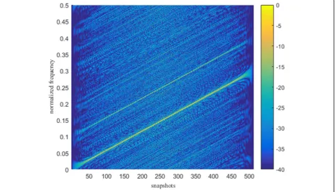
Assume an eight-sensor uniform linear array with a half wavelength separation between each element and an observation duration of 512 samples. The two linear fre-quency modulation signal components are transmitted from two source signals located at anglesθ1andθ2. The

initiated and finished normalized frequencies of the source signal from θ1= 30° are fs1= 0 and fe1= 0.3,

whereas the homologous second frequencies for another source from θ2= 40°are fs2= 0.2 and fe2= 0.5, severally.

WVD is utilized to calculate the time-frequency distribu-tion, and time-frequency averaging is utilized to build the noise subspace. The input SNR ofθ1is 5 dB, whereas

the incoming SNR of θ2 is −5 dB. Figure 1 shows the

time-frequency spectrum of two LFM signals. From

Fig. 1, the auto-term of the weak signal cannot be

obtained on the time-frequency spectrum because of the submergence in noise. However, the cross terms in time-frequency plane can observe the normalized frequencies of which is approximately from 0.1 to

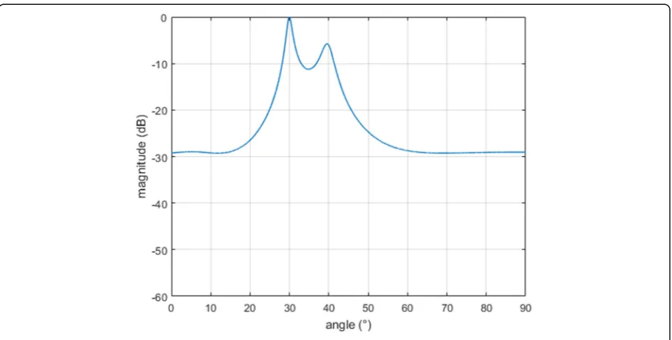
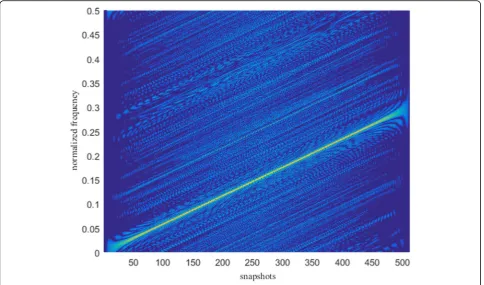
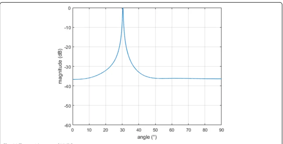
0.4. As shown in Fig. 2, the cross terms are

extracted by the method mentioned above for the DOA estimation of the weak non-stationary signal. The DOA of strong and weak signals is estimated by

cross terms in Fig. 3, which are approximately 30°

and 40°, respectively.

Fig. 3The estimated spatial spectrum

Fig. 5Auto-terms of weak signal

If the SNR difference of the strong and weak signals increases further, the DOA of the weak signal cannot be directly obtained from the cross terms. The input SNR of θ1is 10 dB, whereas the input SNR of θ2is −10 dB.

The cross term is utilized from another perspective. Firstly, the position of the auto-terms of the strong signal and cross terms in the time-frequency domain is estimated. Then the position of the auto-terms of the weak signal is fitted according to the two positions in

order to improve the SNR of the weak non-stationary signals. The spatial time-frequency distribution matrixes are extracted from the position of the weak signal for

the DOA estimation. Figure 4 shows the T-F-spectrum

of two linear frequency modulation signal components. Although the cross terms are no longer obvious on the time-frequency plane, they can also be extracted accord-ing to the characteristics of the matrix. In Fig. 5, the auto-terms of the weak non-stationary signal are fitted

Fig. 6The estimated spatial spectrum

by the method mentioned above for the DOA estima-tion. The DOA of the strong and weak signals is

simul-taneously estimated in Fig. 6, which are approximately

30° and 40°, respectively. The time-frequency-MUSIC technology is realized respectively for two sets of time-frequency points, each one from one source signal.

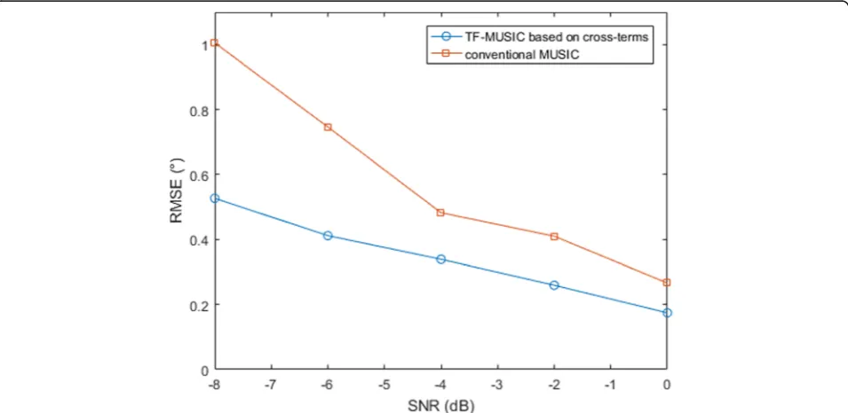
When the incoming SNR ofθ1is 5 dB, the input SNR of

θ2 is from−8 dB to 0 dB. The results were calculated via

averaging 100 Monte Carlo runs. Figure7shows the DOA

estimation root-mean-square error with SNR for traditional MUSIC and time-frequency-MUSIC based on cross-terms. The RMSE of TF-MUSIC based on cross terms is less than that of the conventional MUSIC overall. The advantages of TF-MUSIC based on cross terms in poor SNR conditions become obvious from the figure.

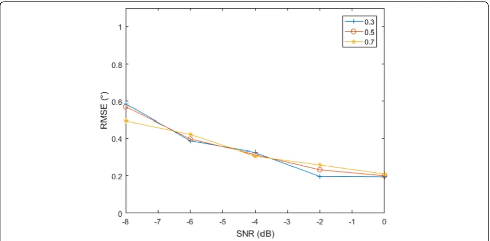
Next, the influence of snapshots on the algorithm is analyzed. With the other simulation conditions men-tioned above unchanged, the number of snapshot is 256,

Fig. 8The RMSE at different snapshots

512, and 1024, respectively. From Fig. 8, the increase in the number of snapshots reduces the RMSE of DOA es-timation. Then, the increase in that will also increase the calculation time. The impact of a small user-defined

positive scalar ε on RMSE is also simulated. With the

512 snapshots, ε is 0.3, 0.5, and 0.7, respectively. From

Fig.9, different values of the same order have little influ-ence on RMSE.

Figures10and11show the estimated spatial spectrum

of TF-MUSIC based on cross terms and the traditional MUSIC where the direction separation is close (θ1= 30°,

θ2= 33°). It is obvious that the source signals can be

Fig. 10The spatial spectra of TF-MUSIC

separated via the time-frequency-MUSIC based on cross terms whereas the conventional MUSIC fails. This is attributed to the combination of time-frequency analysis method and MUSIC algorithm. In the time-frequency MUSIC algorithm, for each signal energy distribution, the MUSIC algorithm is calcu-lated separately, and only a single signal is included in the data covariance matrix. Therefore, two curves are generated and the target with an angle ap-proaching can be distinguished.

5 Conclusions

When the desired weak non-stationary signal may be buried in noise, especially in the condition of low signal-to-noise ratio, it is difficult or almost impossible to ex-tract the auto-term of the weak non-stationary signal. However, the cross terms of the strong and weak non-stationary signal did not decrease significantly, which contain sufficient information of weak non-stationary signal for its DOA estimation. Therefore, in the case that both strong and weak non-stationary signals exist, mean-while, the cross terms of STFDs are used to obtain DOA of the desired weak non-stationary signal in this paper. The DOA estimation root-mean-square error of TF-MUSIC based on cross terms is less than that of conven-tional MUSIC. The DOA of two closely spaced signals is resolved by the TF-MUSIC based on cross terms.

Abbreviations

DOA:Direction of arrival; HT: Hough transform; IF: Instantaneous frequency; LFM: Linear frequency modulation; MUSIC: Multiple signal classification; RMSE: Root-mean-square error; SHR-TFRR: Smoothed high-resolution frequency rate representation; SNR: Signal-to-noise ratio; STFD: Spatial time-frequency distribution; T-F: Time-time-frequency; WVD: Wigner-Ville distribution

Acknowledgements

This work was supported in part by the National Key R&D Program of China under Grant No. 2017YFC1405202, in part by the National Natural Science Foundation of China under Grant No. 61571157 and Grant No. 61571159, in part by the Public Science and Technology Research Funds Projects of Ocean under Grant No. 201505002, in part by the Natural Science Foundation of Shandong Province under Grant No. ZR2018PF001, and in part by the Foundation of Science and Technology on Communication Networks Key Laboratory.

Authors_’contributions

SS and AL conceived and designed the experiments; SS and HY performed the experiments; BL contributed simulation tools; and SS and HY wrote the paper. All authors have read and approved the final manuscript.

Funding

National Key R&D Program of China under Grant No. 2017YFC1405202 is supporting the data acquisition devices and materials; National Natural Science Foundation of China under Grant No. 61571157 and Grant No. 61571159 are supporting the simulations; the Public Science and Technology Research Funds Projects of Ocean under Grant No. 201505002, the Natural Science Foundation of Shandong Province under Grant No. ZR2018PF001, and the Foundation of Science and Technology on Communication Networks Key Laboratory are supporting the data analyses.

Availability of data and materials

The datasets used and/or analyzed during the current study are available from the corresponding author on reasonable request.

Competing interests

The authors declare that they have no competing interests.

Author details

1_{School of Information Science and Engineering, Harbin Institute of}

Technology (Weihai), Weihai, China.2_{Science and Technology on}

Communication Networks Laboratory, Shijiazhuang, China.3_{The 54th}

Research Institute of China Electronics Technology Group Corporation, Shijiazhuang, China.

Received: 10 May 2019 Accepted: 11 September 2019

References

1. Y. Wei, Z. Zhang, T. Yang, inIET International Conference on Wireless IET. Radar signal processing based on a new cross-term reduced Wigner-Ville distribution (2014)

2. Z. Na, Y. Wang, X. Li, Subcarrier allocation based simultaneous wireless information and power transfer algorithm in 5G cooperative OFDM communication systems. Phys. Commun.29, 164–170 (2018)

3. Z. Na, Z. Pan, M. Xiong, et al., Turbo receiver channel estimation for GFDM-based cognitive radio networks. IEEE Access6, 9926–9935 (2018) 4. G. Gaunaurd, H. Strifors, Signal analysis by means of time-frequency

(Wigner-type) distributions-applications to sonar and radar echoes. Proc. IEEE84(9), 1231–1248 (1996)

5. Y. Lai, H. Zhou, Y. Zeng, et al., Quantifying and reducing the DOA estimation error resulting from antenna pattern deviation for direction-finding HF radar. Remote Sens.9(12), 1285 (2017)

6. L. Cohen,Time-frequency analysis(Prentice Hall, Englewood Cliffs, 1995) 7. A. Belouchrani, M. Amin, Blind source separation based on time-frequency

signal representations. IEEE Trans. Signal Process.46(11), 2888_–2897 (2002) 8. Y. Zhang, W. Ma, M. Amin, Subspace analysis of spatial time-frequency

distribution matrices. IEEE Trans. Signal Process.49(4), 747–759 (2001) 9. W. Mu, M. Amin, Y. Zhang, Bilinear signal synthesis in array processing. IEEE

Trans. Signal Process.51(1), 90–100 (2001)

10. A. Erdogan, T. Gulum, L. Durak-Ata, et al., FMCW signal detection and parameter extraction by cross Wigner–Hough transform. IEEE Trans. Aerosp. Electron. Syst.53(1), 334–344 (2017)

11. L. Cohen, Time-frequency distributions-a review. Proc. IEEE77(7), 941_–981 (1989)

12. A. Belouchrani, M. Amin, N. Thirion-Moreau, et al., Source separation and localization using time-frequency distributions: an overview. IEEE Signal Process. Mag.30(6), 97–107 (2013)

13. A. Belouchrani, M. Amin, Time-frequency MUSIC. IEEE Signal Process. Lett.

6(5), 109–110 (2002)

14. S. Barbarossa, A. Zanalda, inIEEE International Conference on Acoustics. A combined Wigner-Ville and Hough transform for cross-terms suppression and optimal detection and parameter estimation (1992)

15. W. Mark, Spectral analysis of the convolution and filtering of non-stationary stochastic processes. J. Sound Vib.11(1), 19–63 (1970)

16. A. Poyil, S. Meethal, inInternational Conference on Industrial Control & Electronics Engineering. Cross-term reduction using wigner hough transform and back estimation (2012)

17. J. Wu, J. Chen, P. Zhong, Time frequency-based blind source separation technique for elimination of cross-terms in Wigner distribution. Electron. Lett.39(5), 475 (2003)

18. J. Guo, X. Zeng, Z. She, Blind source separation based on high-resolution time–frequency distributions. Comput. Electr. Eng.38(1), 175–184 (2012) 19. Q. Li, T. Zhou, W. Wang, inIET International Conference on Wireless. New

method to eliminate cross-term in wigner distribution (2009) 20. L. Zuo, M. Li, Z. Liu, et al., A high resolution time-frequency rate

representation and the cross term suppression. IEEE Trans. Signal Process.

64(10), 2463–2474 (2016)

21. L. Zuo, M. Li, X. Xia, New smoothed time-frequency rate representations for suppressing cross terms. IEEE Trans. Signal Process.65(3), 733-747 (2017) 22. D. Aiordachioaie, T. Popescu, in2017 International Symposium on Signals,

Circuits and Systems (ISSCS). A method to detect and filter the cross terms in the Wigner-Ville distribution (2017), pp. 1–4

24. M. Sandsten, J. Brynolfsson, in2017 25th European Signal Processing Conference (EUSIPCO). Classification of bird song syllables using Wigner-Ville ambiguity function cross-terms (2017), pp. 1739–1743

25. M. Reyna-Carranza, L. Fierro, M. Bravo-Zanoguera, in2012 Pan American Health Care Exchanges.Wigner distribution’s cross terms characterization to detect patterns of ventricular late potentials (2012)

26. J. Jeong, W. Williams, Mechanism of the cross-terms in spectrograms. IEEE Trans. Signal Process.40(10), 2608–2613 (1992)

27. A. Belouchrani, K. Abed-Meraim, M. Amin, et al., inIEEE International Conference on Acoustics. Joint anti-diagonalization for blind source separation (2001), pp. 2789–2792

28. E. Fadaili, N. Moreau, E. Moreau, Nonorthogonal joint diagonalization/zero diagonalization for source separation based on time-frequency distributions. IEEE Trans. Signal Process.55(5), 1673_–1687 (2007)

29. A. Liu, F. Li, S. Chen, et al., in2015 Asia-Pacific Microwave Conference (APMC). DOA estimation based on cross terms of spatial time-frequency distribution matrices (2015)

30. R. Schmidt, Multiple emitter location and signal parameters estimation. IEEE Trans. Antennas Propag.34(3), 276–280 (1986)

31. G. Golub, C. Van Loan, Matrix computations. Math. Gaz.47(5 Series II), 392– 396 (1996)

Publisher’s Note