R E S E A R C H
Open Access
Adaptive link selection algorithms for
distributed estimation
Songcen Xu
1*, Rodrigo C. de Lamare
1,2and H. Vincent Poor
3Abstract
This paper presents adaptive link selection algorithms for distributed estimation and considers their application to wireless sensor networks and smart grids. In particular, exhaustive search-based least mean squares (LMS) / recursive least squares (RLS) link selection algorithms and sparsity-inspired LMS / RLS link selection algorithms that can exploit the topology of networks with poor-quality links are considered. The proposed link selection algorithms are then analyzed in terms of their stability, steady-state, and tracking performance and computational complexity. In comparison with the existing centralized or distributed estimation strategies, the key features of the proposed algorithms are as follows: (1) more accurate estimates and faster convergence speed can be obtained and (2) the network is equipped with the ability of link selection that can circumvent link failures and improve the estimation performance. The performance of the proposed algorithms for distributed estimation is illustrated via simulations in applications of wireless sensor networks and smart grids.
Keywords: Adaptive link selection; Distributed estimation; Wireless sensor networks; Smart grids
1 Introduction
Distributed signal processing algorithms have become a key approach for statistical inference in wireless networks and applications such as wireless sensor networks and smart grids [1–5]. It is well known that distributed pro-cessing techniques deal with the extraction of information from data collected at nodes that are distributed over a geographic area [1]. In this context, for each specific node, a set of neighbor nodes collect their local information and transmit the estimates to a specific node. Then, each spe-cific node combines the collected information together with its local estimate to generate an improved estimate.
1.1 Prior and related work
Several works in the literature have proposed strate-gies for distributed processing which include incremental [1, 6–8], diffusion [2, 9], sparsity-aware [3, 10], and consensus-based strategies [11]. With the incremental strategy, the processing follows a Hamiltonian cycle, i.e., the information flows through these nodes in one direc-tion, which means each node passes the information to its
*Correspondence: [email protected]
1Department of Electronics, University of York, YO10 5DD York, UK Full list of author information is available at the end of the article
adjacent node in a uniform direction. However, in order to determine an optimum cyclic path that covers all nodes (considering the noise, interference, path loss, and chan-nels between neighbor nodes), this method needs to solve an NP-hard problem. In addition, when any of the nodes fails, data communication through the cycle is interrupted and the distributed processing breaks down [1].
In distributed diffusion strategies [2, 10], the neighbors for each node are fixed and the combining coefficients are calculated after the network topology is deployed and starts its operation. One potential risk of this approach is that the estimation procedure may be affected by poorly performing links. More specifically, the fixed neighbors and the pre-calculated combining coefficients may not provide an optimized estimation performance for each specified node because there are links that are more severely affected by noise or fading. Moreover, when the number of neighbor nodes is large, each node requires a large bandwidth and transmit power. In [12, 13], the idea of partial diffusion was introduced for reducing communi-cations between neighbor nodes. Prior work on topology design and adjustment techniques includes the studies in [14–16] and [17], which are not dynamic in the sense that they cannot track changes in the network and mitigate the effects of poor links.
1.2 Contributions
The adaptive link selection algorithms for distributed esti-mation problems are proposed and studied in this chapter. Specifically, we develop adaptive link selection algorithms that can exploit the knowledge of poor links by selecting a subset of data from neighbor nodes. The first approach consists of exhaustive search-based least mean squares (LMS)/ recursive least squares (RLS) link selection (ES-LMS/ES-RLS) algorithms, whereas the second technique is based on sparsity-inspired LMS/RLS link selection (SI-LMS/SI-RLS) algorithms. With both approaches, dis-tributed processing can be divided into two steps. The first step is called the adaptation step, in which each node employs LMS or RLS to perform the adaptation through its local information. Following the adaptation step, each node will combine its collected estimates from its neigh-bors and local estimate, through the proposed adaptive link selection algorithms. The proposed algorithms result in improved estimation performance in terms of the mean square error (MSE) associated with the estimates. In con-trast to previously reported techniques, a key feature of the proposed algorithms is that the combination step involves only a subset of the data associated with the best performing links.
In the ES-LMS and ES-RLS algorithms, we consider all possible combinations for each node with its neigh-bors and choose the combination associated with the smallest MSE value. In the SI-LMS and SI-RLS algo-rithms, we incorporate a reweighted zero attraction (RZA) strategy into the adaptive link selection algorithms. The RZA approach is often employed in applications deal-ing with sparse systems in such a way that it shrinks the small values in the parameter vector to zero, which results in better convergence and steady-state perfor-mance. Unlike prior work with sparsity-aware algorithms [3, 18–20], the proposed SI-LMS and SI-RLS algorithms exploit the possible sparsity of the MSE values asso-ciated with each of the links in a different way. In contrast to existing methods that shrink the signal sam-ples to zero, SI-LMS and SI-RLS shrink to zero the links that have poor performance or high MSE values. By using the SI-LMS and SI-RLS algorithms, the data associated with unsatisfactory performance will be dis-carded, which means the effective network topology used in the estimation procedure will change as well. Although the physical topology is not changed by the proposed algorithms, the choice of the data coming from the neigh-bor nodes for each node is dynamic, leads to the change of combination weights, and results in improved per-formance. We also remark that the topology could be altered with the aid of the proposed algorithms and a feed-back channel which could inform the nodes whether they should be switched off or not. The proposed algorithms are considered for wireless sensor networks and also as a
tool for distributed state estimation that could be used in smart grids.
In summary, the main contributions of this chapter are the following:
• We present adaptive link selection algorithms for distributed estimation that are able to achieve significantly better performance than existing algorithms.
• We devise distributed LMS and RLS algorithms with link selection capabilities to perform distributed estimation.
• We analyze the MSE convergence and tracking performance of the proposed algorithms and their computational complexities, and we derive analytical formulas to predict their MSE performance.
• A simulation study of the proposed and existing distributed estimation algorithms is conducted along with applications in wireless sensor networks and smart grids.
This paper is organized as follows. Section 2 describes the system model and the problem statement. In Section 3, the proposed link selection algorithms are introduced. We analyze the proposed algorithms in terms of their stability, steady-state, and tracking performance and computational complexity in Section 4. The numeri-cal simulation results are provided in Section 5. Finally, we conclude the paper in Section 6.
Notation: We use boldface upper case letters to denote matrices and boldface lower case letters to denote vectors. We use(·)Tand(·)−1to denote the transpose and inverse operators, respectively, (·)H for conjugate transposition and(·)∗for complex conjugate.
2 System model and problem statement
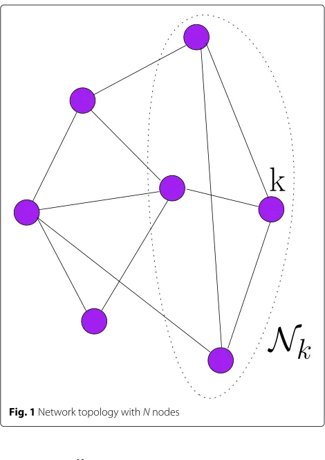
We consider a set of N nodes, which have limited
processing capabilities, distributed over a given geograph-ical area as depicted in Fig. 1. The nodes are connected and form a network, which is assumed to be partially connected because nodes can exchange information only with neighbors determined by the connectivity topology. We call a network with this property a partially connected network whereas a fully connected network means that data broadcast by a node can be captured by all other nodes in the network in one hop [21]. We can think of this network as a wireless network, but our analysis also applies to wired networks such as power grids. In our work, in order to perform link selection strategies, we assume that each node has at least two neighbors.
Fig. 1Network topology withNnodes
dk(i)=ωH0xk(i)+nk(i), i=1, 2,. . .,I, (1)
wherexk(i)is theM×1 random regression input signal vector andnk(i)denotes the Gaussian noise at each node with zero mean and varianceσn2,k. This linear model is able to capture or approximate well many input-output rela-tions for estimation purposes [22], and we assumeI>M. To compute an estimate ofω0in a distributed fashion, we need each node to minimize the MSE cost function [2]
Jk(ωk(i))=Edk(i)−ωHk(i)xk(i) 2
, (2)
whereEdenotes expectation and ωk(i)is the estimated vector generated by nodekat time instanti. Equation (3) is also the definition of the MSE, and the global network cost function could be described as
J(ω)= N
k=1
Edk(i)−ωHxk(i) 2
. (3)
To solve this problem, diffusion strategies have been proposed in [2, 9] and [23]. In these strategies, the esti-mate for each node is generated through a fixed combina-tion strategy given by
ωk(i)=
l∈Nk
cklψl(i), (4)
whereNk denotes the set of neighbors of nodek includ-ing nodekitself,ckl≥0 is the combining coefficient, and ψl(i)is the local estimate generated by nodelthrough its local information.
There are many ways to calculate the combining coeffi-cientcklwhich include the Hastings [24], the Metropolis [25], the Laplacian [26], and the nearest neighbor [27] rules. In this work, due to its simplicity and good per-formance, we adopt the Metropolis rule [25] given by
ckl = ⎧ ⎨ ⎩
1
max{|Nk|,|Nl|}, ifk=lare linked
1−
l∈Nk/k
ckl, fork=l. (5)
where |Nk| denotes the cardinality of Nk. The set of coefficientscklshould satisfy [2]
l∈Nk∀k
ckl=1. (6)
For the combination strategy mentioned in (4), the choice of neighbors for each node is fixed, which results in some problems and limitations, namely:
• Some nodes may face high levels of noise or
interference, which may lead to inaccurate estimates. • When the number of neighbors for each node is high,
large communication bandwidth and high transmit power are required.
• Some nodes may shut down or collapse due to network problems. As a result, local estimates to their neighbors may be affected.
Under such circumstances, a performance degradation is likely to occur when the network cannot discard the contribution of poorly performing links and their associ-ated data in the estimation procedure. In the next section, the proposed adaptive link selection algorithms are pre-sented, which equip a network with the ability to improve the estimation procedure. In the proposed scheme, each node is able to dynamically select the data coming from its neighbors in order to optimize the performance of distributed estimation techniques.
3 Proposed adaptive link selection algorithms
3.1 Exhaustive search–based LMS/RLS link selection The proposed ES-LMS and ES-RLS algorithms employ an exhaustive search to select the links that yield the best performance in terms of MSE. First, we describe how we define the adaptation step for these two strategies. In the ES-LMS algorithm, we employ the adaptation strategy given by
ψk(i)=ωk(i)+μkxk(i)
dk(i)−ωHk(i)xk(i) ∗, (7)
where μk is the step size for each node. In the ES-RLS algorithm, we employ the following steps for the adapta-tion:
whereλis the forgetting factor. Then, we let
Pk(i)=−k1(i) (9)
Following the adaptation step, we introduce the combi-nation step for both the ES-LMS and ES-RLS algorithms, based on an exhaustive search strategy. At first, we intro-duce a tentative set k using a combinatorial approach described by
k ∈2|Nk|\∅, (13)
where the setk is a nonempty set with 2|Nk| elements. After the tentative set k is defined, we write the cost function (2) for each node as
Jk(ψ(i))Edk(i)−ψH(i)xk(i)
is the local estimator andψl(i)is calculated through (7) or (11), depending on the algorithm, i.e., LMS or ES-RLS. With different choices of the setk, the combining coefficientscklwill be re-calculated through (5), to ensure condition (6) is satisfied.
Then, we introduce the error pattern for each node, which is defined as must solve the following optimization problem:
ˆ
k(i)=arg min k∈2Nk\∅|
ek(i)|. (17)
After all steps have been completed, the combination step in (4) is performed as described by
ωk(i+1)=
l∈k(i)
ckl(i)ψl(i). (18)
At this stage, the main steps of the ES-LMS and ES-RLS algorithms have been completed. The proposed ES-LMS and ES-RLS algorithms find the setk(i)that minimizes the error pattern in (16) and (17) and then use this set of nodes to obtainωk(i)through (18).
The ES-LMS/ES-RLS algorithms are briefly summa-rized as follows:
Step 1Each node performs the adaptation through its local information based on the LMS or RLS algorithm.
Step 2Each node finds the best setk(i), which satisfies (17).
Step 3 Each node combines the information obtained from its best set of neighbors through (18).
The details of the proposed ES-LMS and ES-RLS algo-rithms are shown in Algoalgo-rithms 1 and 2. When the ES-LMS and ES-RLS algorithms are implemented in net-works with a large number of small and low–power sensors, the computational complexity cost may become high, as the algorithm in (17) requires an exhaustive search and needs more computations to examine all the possible setsk(i)at each time instant.
Algorithm 1The ES-LMS Algorithm Initialize:ωk(1)=0, fork=1, 2,. . .,N
find all possible sets ofk
Algorithm 2The ES-RLS Algorithm Initialize:ωk(1)=0, fork=1, 2,. . .,N
−1
k (0)=δ−1I,δ=small positive constant For each time instanti=1, 2,. . .,I
For each nodek=1, 2,. . .,N −1
k (i)=λ−1−k1(i−1)
−λ−2−k1(i−1)xk(i)xHk(i)−1(i−1)
1+λ−1xH
k(i)−1(i−1)xk(i)
Pk(i)=−k1(i) kk(i)= λ
−1P k(i)xk(i) 1+λ−1xH
k(i)Pk(i)xk(i) ψk(i)=ωk(i)+k(i)
dk(i)−ωHk(i)xk(i) ∗ Pk(i+1)=λ−1Pk(i)−λ−1k(i)xHk(i)Pk(i) end
For each nodek=1, 2,. . .,N
find all possible sets ofk
ek(i)=dk(i)−
l∈k
ckl(i)ψl(i) H
xk(i)
k(i)=arg min k
|ek(i)| ωk(i+1)=
l∈k(i)
ckl(i)ψl(i)
end end
3.2 Sparsity–inspired LMS/RLS link selection
The ES-LMS/ES-RLS algorithms previously outlined need to examine all possible sets to find a solution at each time instant, which might result in high computa-tional complexity for large networks operating in time-varying scenarios. To solve the combinatorial problem with reduced complexity, we propose the SI-LMS and SI-RLS algorithms, which are as simple as standard diffu-sion LMS or RLS algorithms and are suitable for adaptive implementations and scenarios where the parameters to be estimated are slowly time-varying. The zero-attracting
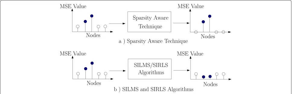
(ZA) strategy, RZA strategy, and zero-forcing (ZF) strat-egy are reported in [3] and [28] as for sparsity-aware techniques. These approaches are usually employed in applications dealing with sparse systems in scenarios where they shrink the small values in the parameter vec-tor to zero, which results in a better convergence rate and a steady-state performance. Unlike existing methods that shrink the signal samples to zero, the proposed SI-LMS and SI-RLS algorithms shrink to zero the links that have poor performance or high MSE values. To detail the novelty of the proposed sparsity-inspired LMS/RLS link selection algorithms, we illustrate the processing in Fig. 2. Figure 2a shows a standard type of sparsity-aware pro-cessing. We can see that, after being processed by a sparsity-aware algorithm, the nodes with small MSE val-ues will be shrunk to zero. In contrast, the proposed SI-LMS and SI-RLS algorithms will keep the nodes with lower MSE values and reduce the combining weight of the nodes with large MSE values as illustrated in Fig. 2b. When compared with the ES-type algorithms, the SI-LMS/RLS algorithms do not need to consider all possible combinations of nodes, which means that the SI-LMS/RLS algorithms have lower complexity. In the following, we will show how the proposed SI-LMS/SI– RLS algorithms are employed to realize the link selection strategy automatically.
In the adaptation step, we follow the same procedure in (7)–(11) as that of the ES-LMS and ES-RLS algorithms for the SI-LMS and SI-RLS algorithms, respectively. Then, we reformulate the combination step. First, we introduce the log-sum penalty into the combination step in (4). Dif-ferent penalty terms have been considered for this task. We have adopted a heuristic approach [3, 29] known as reweighted zero-attracting strategy into the combination step in (4) because this strategy has shown an excellent performance and is simple to implement. The log-sum penalty is defined as:
f1(ek(i))=
l∈Nk
log(1+ε|ekl(i)|), (19)
where the error ekl(i)(l ∈ Nk), which stands for the neighbor node l of node k including node k itself, is defined as
ekl(i)dk(i)−ψHl (i)xk(i) (20)
and ε is the shrinkage magnitude. Then, we introduce
the vector and matrix quantities required to describe the combination step. We first define a vectorckthat contains the combining coefficients for each neighbor of node k
including nodekitself as described by
ck [ckl] , l∈Nk. (21)
Then, we define a matrixk that includes all the esti-mated vectors, which are generated after the adaptation step of SI-LMS and of SI-RLS for each neighbor of nodek
including nodekitself as given by
k[ψl(i)] , l∈Nk. (22)
Note that the adaptation steps of SI-LMS and SI-RLS are identical to (7) and (11), respectively. An error vec-tor eˆk that contains all error values calculated through (20) for each neighbor of nodekincluding nodekitself is expressed by
ˆ
ek [ekl(i)] , l∈Nk. (23)
To devise the sparsity-inspired approach, we have modified the vectoreˆkin the following way:
1. The element with largest absolute value|ekl(i)|ineˆk will be kept as|ekl(i)|.
2. The element with smallest absolute value will be set to−|ekl(i)|. This process will ensure the node with smallest error pattern has a reward on its combining coefficient.
3. The remaining entries will be set to zero.
At this point, the combination step can be defined as [29]
is used to control the algorithm’s shrinkage intensity. We then calculate the partial derivative ofˆek[j]:
∂f1(eˆk,j)
withξminin the denominator of (25), where the parameter ξminstands for the minimum absolute value ofekl(i)inˆek. Then, (25) can be rewritten as
∂f1(eˆk,j) ∂eˆk,j ≈ε
sign(eˆk,j)
1+ε|ξmin|. (26)
At this stage, the log-sum penalty performs shrinkage and selects the set of estimates from the neighbor nodes with the best performance, at the combination step. The function sign(a)is defined as
sign(a)=
a/|a| a=0
0 a=0. (27)
Then, by inserting (26) into (24), the proposed combi-nation step is given by
ωk(i)=
corresponding node has been discarded from the com-bination step. In the following time instant, if this node still has the largest error, there will be no changes in the combining coefficients for this set of nodes.
To guarantee the stability, the parameterρis assumed to be sufficiently small and the penalty takes effect only on the element inekˆ for which the magnitude is comparable to 1/ε[3]. Moreover, there is little shrinkage exerted on the element ineˆk whose|ˆek[j]| 1/ε. The SI-LMS and SI-RLS algorithms perform link selection by the adjust-ment of the combining coefficients through (28). At this point, it should be emphasized that:
• The process in (28) satisfies condition (6), as the penalty and reward amounts of the combining coefficients are the same for the nodes with maximum and minimum error, respectively, and there are no changes for the rest nodes in the set. • When computing (28), there are no matrix–vector
is introduced. As described in (24), only thej th element ofck,eˆkandj th column ofkare used for calculation.
For the neighbor node with the largest MSE value, after the modifications ofeˆk, itsekl(i)value ineˆkwill be a posi-tive number which will lead to the termρεsign(ekˆ,j)
1+ε|ξmin|in (28)
being positive too. This means that the combining coeffi-cient for this node will be shrunk and the weight for this node to build ωk(i) will be shrunk too. In other words, when a node encounters high noise or interference levels, the corresponding MSE value might be large. As a result, we need to reduce the contribution of that node.
In contrast, for the neighbor node with the smallest MSE, as itsekl(i)value ineˆkwill be a negative number, the termρεsign(ekˆ,j)
1+ε|ξmin| in (28) will be negative too. As a result,
the weight for this node associated with the smallest MSE to buildωk(i)will be increased. For the remaining neigh-bor nodes, the entryekl(i)ineˆkis zero, which means the term ρεsign(ˆek,j)
1+ε|ξmin| in (28) is zero and there is no change
for the weights to build ωk(i). The main steps for the proposed SI-LMS and SI-RLS algorithms are listed as follows:
Step 1Each node carries out the adaptation through its local information based on the LMS or RLS algorithm.
Step 2Each node calculates the error pattern through (20).
Step 3Each node modifies the error vectorˆek.
Step 4 Each node combines the information obtained from its selected neighbors through (28).
Algorithm 3The SI-LMS and SI-RLS Algorithms
Initialize:ωk(−1)=0,k=1, 2,. . .,N
P(0)=δ−1I,δ=small positive constant
For each time instanti=1, 2,. . .,I
For each nodek=1, 2,. . .,N
The adaptation step for computingψk(i)
is exactly the same as the ES-LMS and ES-RLS for the SI-LMS and SI-RLS algorithms respectively end
Find the maximum and minimum absolute terms inek
Modifiedˆekasˆek=[0· · ·0,| ekl(i)|
The SI-LMS and SI-RLS algorithms are detailed in Algorithm 3. For the ES-LMS/ES-RLS and SI-LMS/SI-RLS algorithms, we design different combination steps and employ the same adaptation procedure, which means the proposed algorithms have the ability to equip any diffusion-type wireless networks operating with other than the LMS and RLS algorithms. This includes, for example, the diffusion conjugate gradient strategy [30]. Apart from using weights related to the node degree, other signal dependent approaches may also be considered, e.g., the parameter vectors could be weighted according to the signal-to-noise ratio (SNR) (or the noise variance) at each node within the neighborhood.
4 Analysis of the proposed algorithms
In this section, a statistical analysis of the proposed algo-rithms is developed, including a stability analysis and an MSE analysis of the steady-state and tracking perfor-mance. In addition, the computational complexity of the proposed algorithms is also detailed. Before we start the analysis, we make some assumptions that are common in the literature [22].
Assumption I: The weight-error vector εk(i) and the input signal vectorxk(i)are statistically independent, and the weight-error vector for nodekis defined as
εk(i)ωk(i)−ω0, (29)
where ω0 denotes the optimum Wiener solution of the
actual parameter vector to be estimated, and ωk(i) is the estimate produced by a proposed algorithm at time instanti.
Assumption II: The input signal vector xl(i) is drawn from a stochastic process, which is ergodic in the autocor-relation function [22].
Assumption III: TheM×1 vectorq(i)represents a sta-tionary sequence of independent zero mean vectors and positive definite autocorrelation matrixQ=Eq(i)qH(i) , which is independent ofxk(i),nk(i)andεl(i).
Assumption IV (Independence): All regressor input sig-nalsxk(i)are spatially and temporally independent. This assumption allows us to consider the input signal xk(i) independent ofωl(i),l∈Nk.
4.1 Stability analysis
To discuss the stability analysis of the proposed ES-LMS and SI-LMS algorithms, we first substitute (7) into (18) and obtain
By employing Assumption IV, we start with (31) for the ES-LMS algorithm and define the global vectors and matrices:
We also define anN×NmatrixCwhere the
combin-ing coefficients {ckl} correspond to the {l,k} entries of the
matrixCand theNM×NMmatrixCGwith a Kronecker
structure:
CG=C⊗IM (36)
where⊗denotes the Kronecker product.
By insertingel(i+1)=e0−l(i+1)−εHl (i)xl(i+1)into (31), the global version of (31) can then be written as
ε(i+1)=CTG[I−MD(i+1)]ε(i)+CGTMg(i+1), (37)
wheree0−l(i+1)is the estimation error produced by the Wiener filter for nodelas described by
e0−l(i+1)=dl(i)−ωH0xl(i). (38)
If we define
DE[D(i+1)] =diag{R1,. . .,RN}
(39)
and take the expectation of (37), we arrive at
E{ε(i+1)} =CGT[I−MD]E{ε(i)}. (40)
Before we proceed, let us defineX = I−MD. We say that a square matrixXis stable if it satisfiesXi→0 asi→ ∞. A known result in linear algebra states that a matrix is stable if, and only if, all its eigenvalues lie inside the unit circle. We need the following lemma to proceed [9].
Lemma 1.Let CG andX denote arbitrary NM×NM matrices, whereCG has real, non-negative entries, with columns adding up to one. Then, the matrixY =CGTXis stable for any choice ofCGif, and only if,Xis stable.
Proof. Assume thatX is stable, it is true that for every square matrixXand everyα >0, there exists a submulti-plicative matrix norm||·||τthat satisfies||X||τ ≤τ(X)+α,
Since CGT has non-negative entries with columns that add up to one, it is element-wise bounded by unity. This means its Frobenius norm is bounded as well and by the equivalence of norms, so is any norm, in particular ||CGTi||τ. As a result, we have
lim i→∞||Y
i||τ =0, (42)
In view ofLemma 1and (82), we need the matrixI−MD to be stable. As a result, it requiresI−μkRkto be stable for allk, which holds if the following condition is satisfied:
0< μk < 2 λmax(Rk)
(43)
whereλmax(Rk)is the largest eigenvalue of the correlation matrixRk. The difference between the ES-LMS and SI-LMS algorithms is the strategy to calculate the matrixC.
Lemma 1indicates that for any choice ofC, onlyXneeds to be stable. As a result, SI-LMS has the same convergence condition as in (43). Given the convergence conditions, the proposed ES-LMS/ES-RLS and SI-LMS/SI-RLS algo-rithms will adapt according to the network connectivity by choosing the group of nodes with the best available performance to construct their estimates.
4.2 MSE steady-state analysis
In this part of the analysis, we devise formulas to predict the excess MSE (EMSE) of the proposed algorithms. The error signal at nodekcan be expressed as
ek(i)=dk(i)−ωHk(i)xk(i)
=dk(i)−[ω0−εk(i)]Hxk(i) =dk(i)−ωH0xk(i)+εHk(i)xk(i) =e0−k+εkH(i)xk(i).
(44)
WithAssumption I, the MSE expression can be derived as
where tr(·)denotes the trace of a matrix andJmin−kis the
minimum mean square error (MMSE) for nodek[22]:
Jmin−k =σ2 correlation vector between the inputs and the measure-mentdk(i), andKk(i)=E
εk(i)εkH(i) is the weight-error
correlation matrix. From [22], the EMSE is defined as the difference between the mean square error at time instanti
and the minimum mean square error. Then, we can write Jex−k(i)=Jmse−k(i)−Jmin−k
=tr{Rk(i)Kk(i)}.
(47)
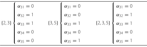
At each time instant, each node will generate data asso-ciated with network covariance matrices Ak with size N×N which reflect the network topology, according to the exhaustive search strategy. In the network covariance matricesAk, a value equal to 1 means nodeskandlare linked and a value 0 means nodeskandlare not linked.
For example, suppose a network has 5 nodes. For node 3, there are two neighbor nodes, namely, nodes 2 and 5. Through Eq. (13), the possible configurations of set3are {3, 2},{3, 5}, and{3, 2, 5}. Evaluating all the possible sets for3, the relevant covariance matricesA3with size 5×5 at time instantiare described in Fig. 3.
Then, the coefficientsαklare obtained according to the covariance matricesAk. In this example, the three sets of αklare respectively shown in Table 1.
The parameters ckl will then be calculated through Eq. (5) for different choices of matricesAkand coefficients αkl. Afterαkl andckl are calculated, the error pattern for each possiblek will be calculated through (16) and the set with the smallest error will be selected according to (17).
With the newly definedαkl, (49) can be rewritten as
εk(i+1)=
Fig. 3Covariance matricesA3for different sets of3
Table 1Coefficientsαklfor different sets of3
whereRl,q(i+1) = E
. To further simplify the analysis, we assume that the samples of the input signalxk(i)are uncorrelated, i.e.,Rk = σx2,kI with σx2,k being the variance. Using the
Fig. 4Covariance matrixA3upon convergence
We assume that the choice of covariance matrixAkfor
node k is fixed upon the proposed algorithms
conver-gence, as a result, the covariance matrixAk is determin-istic and does not vary. In the above example, we assume the choice ofA3is fixed as shown in Fig. 4.
Then the coefficientsαklwill also be fixed and given by ⎧
as well as the parametersckl that are computed using the Metropolis combining rule. As a result, the coefficientsαkl and the coefficientscklare deterministic and can be taken out from the expectation. The MSE is then given by
Jmse−k =Jmin−k+Mσx2,k
For the SI-LMS algorithm, we do not need to consider all possible combinations. This algorithm simply adjusts the combining coefficients for each node with its neighbors in
order to select the neighbor nodes that yield the smallest MSE values. Thus, we redefine the combining coefficients through (28)
ckl−new=ckl−ρε
sign(|ekl|)
1+ε|ξmin| (l∈Nk). (59) For each nodek, at time instanti, after it receives the estimates from all its neighbors, it calculates the error pat-tern ekl(i) for every estimate received through Eq. (20) and finds the nodes with the largest and smallest errors. An error vector eˆk is then defined through (23), which contains all error patternsekl(i)for nodek.
Then a procedure which is detailed after
Eq. (23) is carried out and modifies the error
vec-tor eˆk. For example, suppose node 5 has three
neighbor nodes, which are nodes 3, 6, and 8.
The error vector eˆ5 has the form described by
ˆ
e5= [e53,e55,e56,e58]= [0.023, 0.052,−0.0004,−0.012]. After the modification, the error vectoreˆ5will be edited aseˆ5 = [0, 0.052,−0.0004, 0]. The quantityhkl is then defined as
hkl =ρε sign(|ekl|)
1+ε|ξmin| (
l∈Nk), (60)
and the term ‘error pattern’eklin (60) is from the modified error vectoreˆk.
From [29], we employ the relation E[sign(ekl)]≈ sign(e0−k). According to Eqs. (1) and (38), when the pro-posed algorithm converges at nodekor the time instanti
goes to infinity, we assume that the errore0−kwill be equal to the noise variance at nodek. Then, the asymptotic value
hkl can be divided into three situations due to the rule of the SI-LMS algorithm:
0 for all the remaining nodes.
(61)
Under this situation, after the time instant i goes to infinity, the parametershklfor each neighbor node of node kcan be obtained through (61) and the quantityhklwill be deterministic and can be taken out from the expectation.
Finally, removing the random variablesαkl(i)and insert-ing (59) and (60) into (57), the asymptotic valuesKknfor the SI-LMS algorithm are obtained as in (62).
At this point, the theoretical results are deterministic, and the MSE for SI-LMS algorithm is given by
Jmse−k=Jmin−k+Mσx2,k M
n=1
Kkn(SI-LMS). (63)
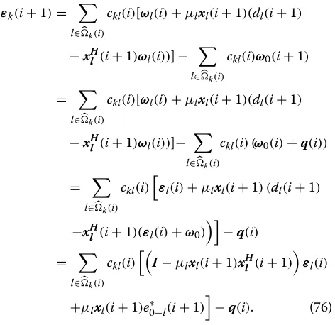
4.2.3 ES-RLS
For the proposed ES-RLS algorithm, we start from (11), after inserting (11) into (18), we have
ωk(i+1)=
l∈k(i)
ckl(i)ψl(i+1)
=
l∈k(i) ckl(i)
ωl(i)+kl(i+1)e∗l(i+1)
=
l∈k(i) ckl(i)
ωl(i)+kl(i+1)(dl(i+1)−xHl (i+1)ωl(i))
. (64)
Then, subtracting theω0from both sides of (48), we arrive at
εk(i+1)=
l∈k(i) ckl(i)
ωl(i)+kl(i+1)(dl(i+1)−xHl (i+1)ωl(i))
−
l∈k(i) ckl(i)ω0
=
l∈k(i) ckl(i)
εl(i)+kl(i+1)
dl(i+1)−xHl (i+1)(εl(i)+ω0)
=
l∈k(i) ckl(i)
I−kl(i+1)xHl (i+1)
εl(i)+kl(i+1)e∗0−l(i+1)
. (65)
Then, with the random variablesαkl(i), (65) can be rewritten as
εk(i+1)=
l∈Nk
αkl(i)ckl(i)
I−kl(i+1)xHl (i+1)
εl(i)+kl(i+1)e∗0−l(i+1)
. (66)
Sincekl(i+1)=−l 1(i+1)xl(i+1)[22], we can modify (66) as
εk(i+1)=
l∈Nk
αkl(i)ckl(i)
I−−l 1(i+1)xl(i+1)xHl (i+1)εl(i)+−l1(i+1)xl(i+1)e∗0−l(i+1)
. (67)
At this point, if we compare (67) with (51), we can find that the difference between (67) and (51) is that the−l 1(i+1) in (67) has replaced theμlin (51). From [22], we also have
E−1 l (i+1)
= 1
i−MR −1
As a result, we can arrive
Due to the structure of the above equations, the approximations and the quantities involved, we can decouple (70) into
Kkn(i+1)=
On the basis of (72), we have that whenitends to infinity, the MSE approaches the MMSE in theory [22].
4.2.4 SI-RLS
Jmse−k=Jmin−k+Mσx2,k M
n=1
Kkn(SI-RLS). (75)
In conclusion, according to (62) and (74), with the help of modified combining coefficients, for the proposed SI-type algorithms, the neighbor node with lowest MSE con-tributes the most to the combination, while the neighbor node with the highest MSE contributes the least. There-fore, the proposed SI-type algorithms perform better than the standard diffusion algorithms with fixed combining coefficients.
4.3 Tracking analysis
In this subsection, we assess the proposed ES-LMS/RLS and SI-LMS/RLS algorithms in a non-stationary environ-ment, in which the algorithms have to track the minimum point of the error performance surface [34, 35]. In the time-varying scenarios of interest, the optimum estimate is assumed to vary according to the modelω0(i+1) = βω0(i)+q(i), whereq(i)denotes a random perturbation [32] andβ = 1 in order to facilitate the analysis. This is typical in the context of tracking analysis of adaptive algorithms [22, 32, 36, 37].
4.3.1 ES-LMS
For the tracking analysis of the ES-LMS algorithm, we employAssumption IIIand start from (48). After subtract-ing theω0(i+1)from both sides of (48), we obtain
UsingAssumption III, we can arrive at
Jex−k(i+1)=tr{Rk(i+1)Kk(i+1)}+tr{Rk(i+1)Q}. (77)
The first part on the right side of (77) has already been obtained in the MSE steady-state analysis part in Section 4 B. The second part can be decomposed as
tr{Rk(i+1)Q} =tr
Exk(i+1)xHk(i+1)Eq(i)qH(i) =Mσx2,ktr{Q}.
(78)
The MSE is then obtained as
Jmse−k=Jmin−k+Mσx2,k
For the SI-LMS recursions, we follow the same procedure as for the ES-LMS algorithm and obtain
Jmse−k=Jmin−k+Mσx2,k
For the SI-RLS algorithm, we follow the same procedure as for the ES-LMS algorithm and arrive at
Jmse−k(i+1)=Jmin−k+Mσx2,k
We start from (75), and after a similar procedure to that of the SI-LMS algorithm, we have
Jmse−k(i+1)=Jmin−k+Mσx2,k In conclusion, for time-varying scenarios, there is only one additional term Mσx2,ktr{Q} in the MSE expression for all algorithms, and this additional term has the same value for all algorithms. As a result, the proposed SI-type algorithms still perform better than the standard diffusion algorithms with fixed combining coefficients, according to the conclusion obtained in the previous subsection.
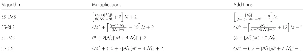
Table 2Computational complexity for the adaptation step per node per time instant
Adaptation method Multiplications Additions
LMS 2M+1 2M
Table 3Computational complexity for the combination step per node per time instant
Algorithms Multiplications Additions
ES–LMS/RLS M(t+1)t!(||NNk|−k|!t)! Mtt!(||NNk|−k|!t)!
SI–LMS/RLS (2M+4)|Nk| (M+2)|Nk|
4.4 Computational complexity
In the analysis of the computational cost of the algo-rithms studied, we assume complex-valued data and first analyze the adaptation step. For both ES-LMS/RLS and SI-LMS/RLS algorithms, the adaptation cost depends on the type of recursions (LMS or RLS) that each strategy employs. The details are shown in Table 2.
In the combination step, we analyze the computational complexity in Table 3. The overall complexity for each algorithm is summarized in Table 4. In the above three tables, t is the number of nodes chosen from|Nk| and
M is the length of the unknown vector ω0. The
pro-posed algorithms require extra computations as compared to the existing distributed LMS and RLS algorithms. This extra cost ranges from a small additional num-ber of operations for the SI-LMS/RLS algorithms to a more significant extra cost that depends on|Nk|for the ES-LMS/RLS algorithms.
5 Simulations
In this section, we investigate the performance of the proposed link selection strategies for distributed estima-tion in two scenarios: wireless sensor networks and smart grids. In these applications, we simulate the proposed link selection strategies in both static and time-varying sce-narios. We also show the analytical results for the MSE steady-state and tracking performances that we obtained in Section 4.
5.1 Diffusion wireless sensor networks
In this subsection, we compare the proposed ES-LMS/ES-RLS and SI-LMS/SI-ES-LMS/ES-RLS algorithms with the diffusion LMS algorithm [2], the diffusion RLS algorithm [38], and the single-link strategy [39] in terms of their MSE performance. A reduced-communication diffusion LMS algorithm with a performance comparable or worse to
the standard diffusion LMS algorithm, which has been reported in [40], may also be considered if a designer needs to reduce the required bandwidth.
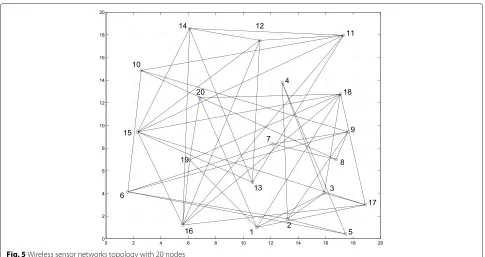
The network topology is illustrated in Fig. 5, and we
employ N = 20 nodes in the simulations. The
aver-age node degree of the wireless sensor network is 5. The length of the unknown parameter vectorω0isM = 10, and it is generated as a complex random vector. The input signal is generated asxk(i)=[xk(i) xk(i−1) . . . xk(i− M+1)] andxk(i)=uk(i)+αkxk(i−1), whereαkis a cor-relation coefficient anduk(i)is a white noise process with varianceσu2,k =1− |αk|2, to ensure the variance ofxk(i)is σ2
x,k =1. Thexk(0)is defined as a Gaussian random num-ber with zero mean and varianceσx2,k. The noise samples are modeled as circular Gaussian noise with zero mean and varianceσn2,k ∈[ 0.001, 0.01]. The step size for the
dif-fusion LMS ES-LMS and SI-LMS algorithms isμ = 0.2.
For the diffusion RLS algorithm, both ES-RLS and SI-RLS, the forgetting factorλis set to 0.97 andδis equal to 0.81. In the static scenario, the sparsity parameters of the
SI-LMS/SI-RLS algorithms are set to ρ = 4 ×10⁻³ and
ε=10. The Metropolis rule is used to calculate the com-bining coefficientsckl. The MSE and MMSE are defined as in (3) and (46), respectively. The results are averaged over 100 independent runs.
In Fig. 6, we can see that the ES-RLS has the best per-formance for both steady-state MSE and convergence rate and obtains a gain of about 8 dB over the standard diffu-sion RLS algorithm. The SI-RLS is worse than the ES–RLS but is still significantly better than the standard diffusion RLS algorithm by about 5 dB. Regarding the complexity and processing time, the SI-RLS is as simple as the stan-dard diffusion RLS algorithm, while the ES-RLS is more complex. The proposed ES-LMS and SI-LMS algorithms are superior to the standard diffusion LMS algorithm.
In the time-varying scenario, the sparsity parameters of the SI-LMS and SI-RLS algorithms are set toρ=6×10⁻³
and ε = 10. The unknown parameter vector ω0 varies
according to the first-order Markov vector process:
ω0(i+1)=βω0(i)+q(i), (83)
whereq(i)is an independent zero mean Gaussian vector process with varianceσq2=0.01 andβ=0.9998.
Table 4Computational complexity per node per time instant
Algorithm Multiplications Additions
ES-LMS t(!t(+|N1)k|−|Nk|t)!!+8M+2 (t−1)|!N(|Nk|!k|−t)!+8M
ES-RLS 4M2+(t+1)|Nk|!
t!(|Nk|−t)!+16
M+2 4M2+ |Nk|!
(t−1)!(|Nk|−t)!+12
M−1
SI-LMS (8+2|Nk|)M+4|Nk| +2 (8+ |Nk|)M+2|Nk|
SI-RLS 4M2+(16+2|N
Fig. 5Wireless sensor networks topology with 20 nodes
Figure 7 shows that, similarly to the static scenario, the ES-RLS has the best performance and obtains a 5 dB gain over the standard diffusion RLS algo-rithm. The SI-RLS is slightly worse than the ES-RLS but is still better than the standard diffusion RLS algorithm by about 3 dB. The proposed ES-LMS and SI-LMS algorithms have the same advantage over
the standard diffusion LMS algorithm in the time-varying scenario. Notice that in the scenario with large |Nk|, the proposed SI-type algorithms still have a bet-ter performance when compared with the standard techniques.
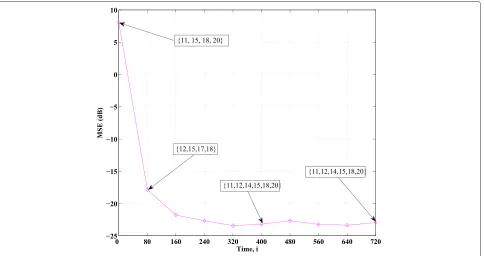
To illustrate the link selection for the ES-type algo-rithms, we provide Figs. 8 and 9. From these two figures,
Fig. 7Network MSE curves in a time-varying scenario
we can see that upon convergence, the proposed algo-rithms converge to a fixed selected set of linksk.
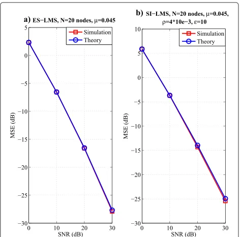
5.2 MSE analytical results
The aim of this section is to validate the analytical results obtained in Section 4. First, we verify the MSE steady-state performance. Specifically, we compare the analytical
results in (58), (63), (73) and (75) to the results obtained by simulations under different SNR values. The SNR indicates the input signal variance to noise variance ratio. We assess the MSE against the SNR, as shown in Figs. 10 and 11. For ES-RLS and SI-RLS algorithms, we use (73) and (75) to compute the MSE after convergence. The results show that the analytical curves coincide with those
Fig. 9Link selection state for node 16 with ES-LMS in a time-varying scenario
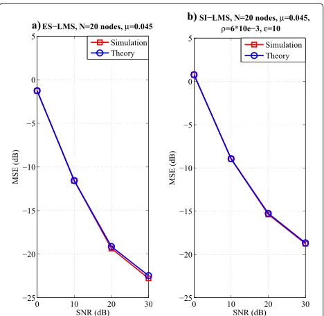
obtained by simulations, which indicates the validity of the analysis. We have assessed the proposed algorithms with SNR equal to 0, 10, 20, and 30 dB, respectively, with 20 nodes in the network. For the other parameters, we follow the same definitions used to obtain the network MSE curves in a static scenario. The details have been shown on the top of each subfigure in Figs. 10 and 11. The
Fig. 10 a–bMSE performance against SNR for ES-LMS and SI-LMS
theoretical curves for ES-LMS/RLS and SI-LMS/RLS are all close to the simulation curves.
The tracking analysis of the proposed algorithms in a time-varying scenario is discussed as follows. Here, we verify that the results in (79), (80), (81), and (82) of the subsection 4.3 can provide a means of estimating the MSE. We consider the same model as in (83), but with
Fig. 12 a–bMSE performance against SNR for ES-LMS and SI-LMS in a time-varying scenario
β set to 1. In the next examples, we employ N = 20
nodes in the network and the same parameters used to obtain the network MSE curves in a time-varying sce-nario. A comparison of the curves obtained by simula-tions and by the analytical formulas is shown in Figs. 12 and 13. From these curves, we can verify that the gap between the simulation and analysis results are extraor-dinary small under different SNR values. The details of
Fig. 13 a–bMSE performance against SNR for ES-RLS and SI-RLS in a time-varying scenario
the parameters are shown on the top of each subfigure in Figs. 12 and 13.
5.3 Smart Grids
The proposed algorithms provide a cost-effective tool that could be used for distributed state estimation in smart grid applications. In order to test the proposed algorithms in a possible smart grid scenario, we consider the IEEE 14-bus system [41], where 14 is the number of substations. At every time instanti, each busk,k = 1, 2,. . ., 14, takes a scalar measurementdk(i)according to
dk(i)=Xk(ω0(i))+nk(i), k=1, 2,. . ., 14, (84)
whereω0(i)is the state vector of the entire interconnected system andXk(ω0(i))is a nonlinear measurement func-tion of busk. The quantitynk(i)is the measurement error with mean equal to zero and which corresponds to busk.
Initially, we focus on the linearized DC state estimation problem. The state vector ω0(i) is taken as the voltage phase angle vectorω0for all busses. Therefore, the non-linear measurement model for state estimation (84) is approximated by
dk(i)=ω0Hxk(i)+nk(i), k=1, 2,. . ., 14, (85)
wherexk(i)is the measurement Jacobian vector for busk. Then, the aim of the distributed estimation algorithm is to compute an estimate ofω0, which can minimize the cost function given by
Jk(ωk(i))=E|dk(i)−ωHk(i)xk(i)|2. (86) We compare the proposed algorithms with the M-CSE algorithm [4], the single-link strategy [39], the standard diffusion RLS algorithm [38], and the standard diffusion LMS algorithm [2] in terms of MSE performance. The MSE comparison is used to determine the accuracy of
Fig. 15MSE performance curves for smart grids
the algorithms and compare the rate of convergence. We define the IEEE 14-bus system as in Fig. 14.
All busses are corrupted by additive white Gaussian noise with varianceσn2,k ∈[0.001, 0.01]. The step size for the standard diffusion LMS [2], the proposed ES-LMS, and SI-LMS algorithms is 0.15. The parameter vectorω0is set to an all-one vector. For the diffusion RLS, ES-RLS, and SI-RLS algorithms, the forgetting factorλis set to 0.945 andδis equal to 0.001. The sparsity parameters of the SI-LMS/RLS algorithms are set toρ=0.07 andε=10. The results are averaged over 100 independent runs. We simu-late the proposed algorithms for smart grids under a static scenario.
From Fig. 15, it can be seen that ES-RLS has the best performance and significantly outperforms the standard diffusion LMS [2] and theM–CSE [4] algorithms. The ES-LMS is slightly worse than the ES-RLS, which out-performs the remaining techniques. The SI-RLS is worse than the ES-LMS but is still better than SI-LMS, while the SI-LMS remains better than the diffusion RLS, LMS, and M-CSEalgorithms and the single-link strategy.
6 Conclusions
In this paper, we have proposed the ES-LMS/RLS and SI-LMS/RLS algorithms for distributed estimation in appli-cations such as wireless sensor networks and smart grids. We have compared the proposed algorithms with existing methods. We have also devised analytical expressions to predict their MSE steady-state performance and tracking behavior. Simulation experiments have been conducted
to verify the analytical results and illustrate that the pro-posed algorithms significantly outperform the existing strategies, in both static and time-varying scenarios, in examples of wireless sensor networks and smart grids.
Competing interests
The authors declare that they have no competing interests.
Acknowledgements
This research was supported in part by the US National Science Foundation under Grants CCF-1420575, CNS-1456793, and DMS-1118605.
Part of this work has been presented at the 2013 IEEE International Conference on Acoustics, Speech, and Signal Processing, Vancouver, Canada and 2013 IEEE International Workshop on Computational Advances in Multi-Sensor Adaptive Processing, Saint Martin.
The authors wish to thank the anonymous reviewers, whose comments and suggestions have greatly improved the presentation of these results.
Author details
1Department of Electronics, University of York, YO10 5DD York, UK.2CETUC,
PUC-Rio, Rio de Janeiro, Brazil.3Department of Electrical Engineering, Princeton University, 08544 Princeton NJ, USA.
Received: 26 May 2015 Accepted: 23 September 2015
References
1. CG Lopes, AH Sayed, Incremental adaptive strategies over distributed networks. IEEE Trans. Signal Process.48(8), 223–229 (2007) 2. CG Lopes, AH Sayed, Diffusion least-mean squares over adaptive
networks: Formulation and performance analysis. IEEE Trans. Signal Process.56(7), 3122–3136 (2008)
3. Y Chen, Y Gu, AO Hero, inProc. IEEE International Conference on Acoustics, Speech and Signal Processing. Sparse LMS for system identification, (2009), pp. 3125–3128
5. Y-H Huang, S Werner, J Huang, VG N. Kashyap, State estimation in electric power grids: meeting new challenges presented by the requirements of the future grid. IEEE Signal Process. Mag.29(5), 33–43 (2012)
6. D Bertsekas, A new class of incremental gradient methods for least squares problems. SIAM J. Optim.7(4), 913–926 (1997)
7. A Nedic, D Bertsekas, Incremental subgradient methods for nondifferentiable optimization. SIAM J. Optim.12(1), 109–138 (2001) 8. MG Rabbat, RD Nowak, Quantized incremental algorithms for distributed
optimization. IEEE J. Sel. Areas Commun.23(4), 798–808 (2005) 9. FS Cattivelli, AH Sayed, Diffusion LMS strategies for distributed estimation.
IEEE Trans. Signal Process.58, 1035–1048 (2010)
10. PD Lorenzo, S Barbarossa, AH Sayed, inProc. IEEE International Conference on Acoustics, Speech, and Signal Processing. Sparse diffusion LMS for distributed adaptive estimation, (2012), pp. 3281–3284
11. G Mateos, ID Schizas, GB Giannakis, Distributed Recursive Least-Squares for Consensus-Based In-Network Adaptive Estimation. IEEE Trans. Signal Process.57(11), 4583–4588 (2009)
12. R Arablouei, K Do ˇgançay, S Werner, Y-F Huang, Adaptive distributed estimation based on recursive least-squares and partial diffusion. IEEE Trans. Signal Process.62, 3510–3522 (2014)
13. R Arablouei, S Werner, Y-F Huang, K Do ˇgançay, Distributed least mean–square estimation with partial diffusion. IEEE Trans. Signal Process.
62, 472–484 (2014)
14. CG Lopes, AH Sayed, inProc. IEEE International Conference on Acoustics, Speech and Signal Processing. Diffusion adaptive networks with changing topologies (Las Vegas, 2008), pp. 3285–3288
15. B Fadlallah, J Principe, inProc. IEEE International Joint Conference on Neural Networks. Diffusion least-mean squares over adaptive networks with dynamic topologies, (2013), pp. 1–6
16. S-Y Tu, AH Sayed, On the influence of informed agents on learning and adaptation over networks. IEEE Trans. Signal Process.61, 1339–1356 (2013) 17. T Wimalajeewa, SK Jayaweera, Distributed node selection for sequential
estimation over noisy communication channels. IEEE Trans. Wirel. Commun.9(7), 2290–2301 (2010)
18. RC de Lamare, R Sampaio-Neto, Adaptive reduced-rank processing based on joint and iterative interpolation, decimation and filtering. IEEE Trans. Signal Process.57(7), 2503–2514 (2009)
19. RC de Lamare, PSR Diniz, Set-membership adaptive algorithms based on time-varying error bounds for CDMA interference suppression. IEEE Trans. Vehi. Techn.58(2), 644–654 (2009)
20. L Guo, YF Huang, Frequency-domain set-membership filtering and its applications. IEEE Trans. Signal Process.55(4), 1326–1338 (2007) 21. A Bertrand, M Moonen, Distributed adaptive node–specific signal
estimation in fully connected sensor networks–part II: simultaneous and asynchronous node updating. IEEE Trans. Signal Process.58(10), 5292–5306 (2010)
22. S Haykin,Adaptive Filter Theory, 4th edn. (Prentice Hall, Upper Saddle River, NJ, USA, 2002)
23. L Li, JA Chambers, inProc. IEEE/SP 15th Workshop on Statistical Signal Processing. Distributed adaptive estimation based on the APA algorithm over diffusion networks with changing topology, (2009), pp. 757–760 24. X Zhao, AH Sayed, Performance limits for distributed estimation over LMS
adaptive networks. IEEE Trans. Signal Process.60(10), 5107–5124 (2012) 25. L Xiao, S Boyd, Fast linear iterations for distributed averaging. Syst. Control
Lett.53(1), 65–78 (2004)
26. R Olfati-Saber, RM Murray, Consensus problems in networks of agents with switching topology and time-delays. IEEE Trans. Autom. Control.49, 1520–1533 (2004)
27. A Jadbabaie, J Lin, AS Morse, Coordination of groups of mobile autonomous agents using nearest neighbor rules. IEEE Trans. Autom. Control.48(6), 988–1001 (2003)
28. R Meng, RC de Lamare, VH Nascimento, inProc. Sensor Signal Processing for Defence. Sparsity-aware affine projection adaptive algorithms for system identification (London, UK, 2011)
29. Y Chen, Y Gu, A Hero, Regularized least-mean-square algorithms. Tech. Rep. AFOSR (2010)
30. S Xu, RC de Lamare, inProc. Sensor Signal Processing for Defence. Distributed conjugate gradient strategies for distributed estimation over sensor networks (London, UK, 2012)
31. F Cattivelli, AH Sayed, Diffusion strategies for distributed Kalman filtering and smoothing. IEEE Trans. Autom. Control.55(9), 2069–2084 (2010)
32. AH Sayed,Fundamentals of adaptive filtering. (John Wiley&Sons, Hoboken, NJ, USA, 2003)
33. T Kailath, AH Sayed, B Hassibi,Linear Estimation. (Prentice-Hall, Englewood Cliffs, NJ, USA, 2000)
34. RC de Lamare, PSR Diniz, Blind adaptive interference suppression based on set-membership constrained constant-modulus algorithms with dynamic bounds. IEEE Trans. Signal Process.61(5), 1288–1301 (2013) 35. Y Cai, RC de Lamare, Low-complexity variable step-size mechanism for
code-constrained constant modulus stochastic gradient algorithms applied to CDMA interference suppression. IEEE Trans. Signal Process.
57(1), 313–323 (2009)
36. B Widrow, SD Stearns,Adaptive signal processing. (Prentice-Hall, Englewood Cliffs, NJ, USA, 1985)
37. E Eweda, Comparison of RLS, LMS, and sign algorithms for tracking randomly time-varying channels. IEEE Trans. Signal Process.42, 2937–2944 (1994)
38. FS Cattivelli, CG Lopes, AH Sayed, Diffusion recursive least-squares for distributed estimation over adaptive networks. IEEE Trans. Signal Process.
56(5), 1865–1877 (2008)
39. X Zhao, AH Sayed, inProc. IEEE International Conference on Acoustics, Speech and Signal Processing. Single-link diffusion strategies over adaptive networks, (2012), pp. 3749–3752
40. R Arablouei, S Werner, K Do ˇgançanay, Y-F Huang, Analysis of a
reduced-communication diffusion LMS algorithm. Signal Processing.117, 355–361 (2015)
41. A Bose, Smart transmission grid applications and their supporting infrastructure. IEEE Trans. Smart Grid.1(1), 11–19 (2010)
Submit your manuscript to a
journal and benefi t from:
7Convenient online submission
7Rigorous peer review
7Immediate publication on acceptance
7Open access: articles freely available online
7High visibility within the fi eld
7Retaining the copyright to your article