On the calibration of a vectorial
4He
pumped magnetometer
O. Gravrand1, A. Khokhlov2,3, J. L. Le Mou¨el3, and J. M. L´eger1
1Laboratoire d’Electronique et de Technique d’Instrumentation, Commissariat `a l’´energie atomique, referred to later on as CEA/LETI Grenoble - 17 rue des martyrs - 38054 Grenoble cedex 9, France
2International Institute of Earthquake Prediction Theory and Mathematical Geophysics 79, b2, Warshavskoe shosse 113556 Moscow, Russia 3Institut de Physique du Globe de Paris, 4, Place Jussieu, 75252, Paris, France
(Received October 30, 2000; Revised April 17, 2001; Accepted May 28, 2001)
The prototype of a 4Hepumped vector magnetometer is presented. Large auxiliary coils systems used in
pre-viously developed apparatus to allow vector measurements from a scalar (atomic or nuclear resonance) sensor are replaced by a light triaxial modulation system associated with advanced techniques of signal processing. The performances of the helium scalar sensor are first briefly recalled; then the principle of the vector measurement, obtained by adding three (approximately) orthogonal modulations of different frequencies (all of the order of 10 Hz) is explained. Afterwards a second part of the paper is devoted to the calibration process, and a first estimate of the performances of the vector magnetometer is obtained. They confirm that this instrument could be a good candidate for an automatic absolute magnetic observatory: after the calibration process completion and a proper installation, it would provide by itself the absolute value of three orthogonal components of the field. In addition to that, the4Hevector magnetometer appears to be also promising for space applications.
1.
Introduction
The idea of designing a vector magnetometer based on an atomic or nuclear resonance sensor—delivering by itself only measurements of intensity of the magnetic field—by adding auxiliary equipment is not new. A pioneering re-alization was the automatic standard magnetic observatory (ASMO) of L. R. Alldredge (1960–1964) (Alldredge, 1960; Alldredge and Saldukas, 1964) built around a rubidium va-por self oscillating magnetometer. The auxiliary equipment consisted of two mutually perpendicular pairs of coils which controlled bias fields in a plane perpendicular to the mean magnetic field vector. Such an instrument was installed at Fredericksburg observatory.
Following it, several “absolute” vector magnetometers were built from a proton or atomic resonance sensor and a system of coils. Some of them were commercialized (such as the ELSEC), many were constructed by scientists work-ing in scientific institutions and magnetic observatories (as the big coils system of Kasmmer in Kakioka observatory). In fact, most of these magnetometers were used only for sporadic absolute measurements the way the classical induc-tometers and theodolites (with the Gauss-Lamont method to measure the horizontal component) used to be. Their perfor-mances, according to our experience, were reasonably good (except for the measurement of the component perpendic-ular to the geographic meridian). The introduction in the early 80’s of D.I. flux (D for declination, I for inclination, flux for fluxgate) theodolite, very easy to handle, coupled with a proton or atomic resonance scalar sensor, reduced the
Copy right c The Society of Geomagnetism and Earth, Planetary and Space Sciences (SGEPSS); The Seismological Society of Japan; The Volcanological Society of Japan; The Geodetic Society of Japan; The Japanese Society for Planetary Sciences.
interest for such systems.
In any case, the objective of an automatic observatory combining—according to the views of Alldredge—“the measurement of magnetic variations and absolute values”, has been abandoned almost everywhere. The main reason is that, without an independent absolute control, the systems made of a scalar sensor and a coils system are subject to im-portant drifts. And, as soon as regular independent absolute measurements are required, it is much more practical to use fluxgate (for example) variometers.
Nevertheless, the project of an automatic (standard) mag-netic observatory has conserved all its interest. The number of magnetic observatories operated at the Earth’s surface is dramatically insufficient, with furthermore a very poor geo-graphical distribution (which raises the question of sea bot-tom observatories). The availability of an aubot-tomatic obser-vatory would greatly help to improve the situation. Let us recall the performances that such an equipment should reach (adopting Intermagnet, Trigg and Coles (1999) claimed standards for classical observatories): provide the absolute values of three components of the magnetic field with an accuracy of the order of 1 nT, without independent abso-lute control (or more probably with a control by indepen-dent long spaced absolute measurements, for example once a year; no strict rule is to be given there).
The present helium pumped vector magnetometer chal-lenges such an objective. Its main originality is that it re-places complicated mechanical devices such as large coils systems with drift prone axes by a light triaxial modulation system associated with advanced techniques of signal pro-cessing. Furthermore, whereas ASMO was a pulsed mag-netometer, the helium magnetometer is a continuous
950 O. GRAVRANDet al.: ON THE CALIBRATION OF A VECTORIAL4HePUMPED MAGNETOMETER
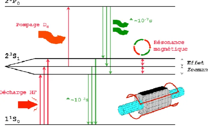
Fig. 1. 4Heenergy diagram.
ment, which allows a perfect control of the noise spectrum and prevents from aliasing problems.
Efforts to conceive and realize automatic magnetic obser-vatories (with the objective of requesting only long spaced absolute measurements) are unfortunately rather few. Let us quote the system presently developed at the Institut Royal m´et´eorologique in Belgium (Rasson, 1994) which consists of an automated DI flux theodolite intended indeed for mak-ing unattended measurements of the declination and inclina-tion in an observatory environment. Rasson’s magnetome-ter is also planned for sea-bottom observations. Let us quote also theIDsystem (delta I delta D) presently developed in Hungary, France and US, although its objective is more to allow interpolations between classical absolute measure-ments than to construct a genuine automatic observatory.
2.
Principle of the Helium Vector Magnetometer
The magnetometer which will be described in this paper, together with its calibration technique—which we will fo-cus on—intends to provide an absolute measurement of the intensity of the magnetic field together with its components along three stable axes simultaneously and at the same place. This type of sensor delivers redundant information in the sense that the calculated modulus obtained thanks to the vec-tor measurements can be compared with the direct intensity (scalar) measurement. The idea of this paper is to use this re-dundancy to estimate the calibration parameters needed for the vector measurement. This method has been applied for a long time to calibrate space magnetometers (Merayoet al., 2000); it will be used here in an original way.
2.1 The scalar helium pumped magnetometer.
Princi-ples of operation and description
Over the past few years, CEA/LETI has been involved in the development of an isotropic4Hepumped magnetometer
(Guttinet al., 1993).
Helium magnetometers are based on an electronic
mag-netic resonance whose effects are amplified by a laser pump-ing process. The first step is to excite a fraction of the he-lium atoms to the 23S
1metastable state by means of a high
frequency discharge. This energy level it split by the static magnetic field Ho into three Zeeman sublevels (Colegrove
and Schearer, 1961). The measurement of their energy sep-aration provides then a very convenient means to determine the earth field.
This is performed thanks to a magnetic resonance exper-iment. Hence, the second step is to induce transitions be-tween the sublevels in order to detect the resonance. If the applied radiofrequency field matches the Larmor frequency of the Zeeman sublevels, transitions between these sublevels occur and tend to equalize their populations. However, the resonance signal amplitude is very low since at thermal equi-librium the sublevels are almost equally populated and no significant change subsequently results from the resonance. So the third step is to modify the repartition of the atoms within the three sublevels (alignment or polarization of the metastable state). This is accomplished by optically pump-ing helium atoms with a tuned laser: atoms in the 23S
1
metastable state absorb the laser light with different prob-abilities for each sublevel and are thus selectively excited to the 23P
0 state (Fig. 1). From there, they undergo a
spon-taneous emission back to the metastable state. Thanks to this process, the resonance signal amplitude is enhanced by several orders of magnitude.
The resonance can be detected by monitoring the trans-mitted laser intensity: when the resonance condition is met, the polarization of the metastable state created as a result of the optical pumping process is reduced by the RF field so that the helium cell transparency decreases. The RF field frequency is then phase locked by an electronic loop to the Larmor frequency, resulting in a field/frequency transducer which can be used as a high sensitivity magnetometer.
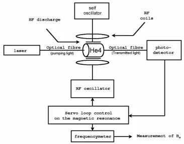
illus-Fig. 2. Architecture of the scalar4Hepumped magnetometer.
trated by Fig. 2. The apparatus has the following perfor-mances.
a) Very high sensitivity: of the order of 1 pT/√Hz. The r.m.s noise results from the integration of the noise density over the sensor bandwith (see below):
B (nTrms) = √B × B (nT/√Hz); takingB =
1 Hz, a 1 pT/√Hz noise density is equivalent to a 1 pT noise level.
b) Bandwidth: DC to 200–300 Hz.
c) Absolute accuracy: better than 100 pT. The absolute accuracy takes into account various phenomena such as thermal drift, uncertainties on the exact value of the metastable helium gyromagnetic ratio, measurement offsets induced by the sensor head materials. For com-parison, the NMR scalar magnetometers which have been developed by LETI for the Ørsted and Champ satellite missions were specified for an absolute accu-racy of±250 pT.
d) Range of measured field: [5μT, 100μT] with no signal to noise ratio variation.
2.2 Principle of the vector measurement
Thanks to the combination of characteristics a and b, it is possible to design a continuous vector magnetometer by adding three orthogonal modulationsβ1,β2,β3(1,2,3 refer to the axes of the triaxial coil system{e1,e2,e3}used to
gen-erate these modulations) to the geomagnetic fieldBseen by the sensing cell. Characteristics a and b are indeed
neces-sary to design a continuous vector magnetometer based on a scalar sensor. It is indeed requested to
i) use permanent modulations to avoid aliasing,
ii) make sure that the magnetometer adequately follows the magnetic field variations resulting from these mod-ulations; this constraint implies a high bandwith of the scalar sensor,
iii) use a very sensitive scalar magnetometer to obtain good vector measurements since these latter measurements are much less sensitive than the scalar ones (see expla-nation below formula (2)).
The scalar magnetometer measures the modulus of the re-sulting field:
|Btot| = B+
3
j=1
βjcos(ω jt)ej
(1)
whereωj are the modulation pulsations.
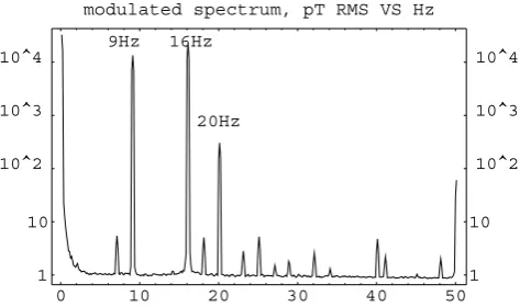
The vector measurement is obtained by processing the 32 bits numerical output of the scalar measurement (1). This scalar output contains several spectral components as can be seen on Fig. 3:
• a DC component
• principal harmonics atωj pulsations
952 O. GRAVRANDet al.: ON THE CALIBRATION OF A VECTORIAL4HePUMPED MAGNETOMETER modulated spectrum, pT RMS VS Hz
9Hz 16Hz
20Hz
Fig. 3. Spectral density of the signal obtained with the modulated scalar
4Hepumped magnetometer when the sensor is submitted to the three
modulations (modulationsωjat 9 Hz, 16 Hz and 20 Hz).
In the hypothesis of a slowly varying magnetic field B
(varying with time constants small with respect to the mod-ulation frequencies), and modmod-ulation amplitudes of the or-der of 10−3|B|, the DC component can be interpreted as a
measurement of the magnetic field modulus b = |B|(but see Subsection 2.3), and principal harmonicsh1,h2 andh3
(which denote the measured amplitudes) are proportional to the projections of the vectorB onto the 3 axes of modula-tion:
hj =β
j(B· e j)
b (2)
A first objective of the vector magnetometer is to retrieve
B· ej, (j = 1,2,3) from the scalar data b,hj. From the
above formula (2), this is possible once theβj are known.
Attention has to be paid to the fact that the projectionB· ej
will be deduced through a very high noise amplification fac-torb/β ∼= 103: a noise of 1 pT/√Hz onhj will be
inter-preted as a noise of 1 nT/√Hz on the projection. Therefore, very high precision and sensitivity are needed in the mea-surements of thehj’s. Moreover, ifβj fluctuates of say 10 ppm, this will be interpreted by the vector instrument as a 10 ppm fluctuation ofBj = B·ej. Modulation amplitudes must
therefore be well known and controlled in order to make ac-curate measurements. To avoid fluctuations, special care has been taken to realize the modulation coils set and the modu-lation current generator:
• High purity silica has been used for the coils supports, resulting in a mechanical stability of 5×10⁻⁷K−1
• A highly stable electronics has been designed (with a temperature dependence smaller than 10−6K−1)
In any case, the direct knowledge of the coils transfer functions and of the electrical current source characteristics does not provide theβjwith a sufficient accuracy: a calibra-tion is necessary.
ProjectionsB·ejon the sensor frame axes{e1,e2,e3}will
be then available. But again theej are only approximately
known. In order to take benefit of the 1 nT/√Hz noise on the vector measurement (see above), a precision of 10−5r ad
is required on the modulation directionsej determination,
which cannot be guaranteed by construction. A calibration process is once more necessary to determine theej with the
required precision. In fact, concerning the directional cali-bration in the present paper, we will limit ourselves to the accurate determination of the angles between the axes of the sensor frame (see Section 4).
It might be said that we are faced with the need of a “strain” calibration (theβj) and a directional calibration (the
ej). Before presenting in detail the calibration process, let
us note that the vector measurement delivered by such a sen-sor is free of offsets, which is an important advantage over fluxgate directional magnetometers (Nielsen et al., 1995), for which in fact three additional parameters must also be estimated during the calibration process.
2.3 Consequence of the modulations on the scalar
ab-solute measurement
The DC component of the output is taken as the mea-surement of the modulusb = |B|. Note nevertheless that any modulation not aligned with the static magnetic fieldB
induces an aliasing of the second order harmonics (whose amplitudes are notedh2j, 2j standing for the double of the
modulation frequency on the j axis) onto the continuous level DC; therefore, in fact:
DC=b−
In the case of a perfect triorthogonal coils set and identical modulation amplitudes (β1=β2=β3=β) along the three
axes, the aliasing term remains independent of the direction of the field. Moreover, its magnitude is very low in a 50μT magnetic field:
In practice, skewness in the axes and differences between the
βj’s may occur and thus may cause the aliasing to vary with
the direction ofB. However, the average value of this error is very small (25 pT) and its variations will be smaller by sev-eral orders of magnitude, and therefore negligible (remem-ber that the values ofβjhave to be stable up to 1 ppm·K−1).
Actually this aliasing is safely neglected in the calibration algorithm. But one must keep its existence in mind as it in-duces a systematic error (which can however be easily sys-tematically corrected if necessary), on the scalar absolute measurement.
3.
Description of the Calibration Problem
3.1 Notations
Let us consider the magnetic field vectorBdefined in the 3-dimensional real vector spaceR3equipped with a
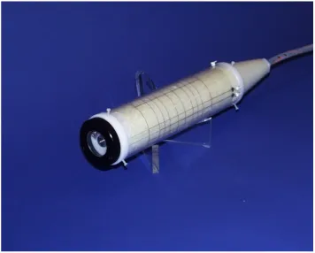
Fig. 4. Triaxial vector helium pumped sensor developed at LETI. (length 30 cm; diameter 6 cm)
for example the geophysical frame: horizontal North, hori-zontal East, downwards vertical).
We list the notations in use for measured and unknown quantities:
b = |B|is the measurement of the magnetic field modulus (neglecting the second order aliasing);
ejis the unit vector of the corresponding modulation
direc-tion (unknown);
βj denotes the modulation amplitude (unknown positive
value) along the corresponding direction; = ∗ is the matrix of modulation amplitudes (∗is for transpo-sition):
=
β1 0 0
0 β2 0 0 0 β3
(4)
Bj = B· e
j is the projection ofBon the directionej; we
denoteB the triplet(B1,B2,B3) of such projections
(unknown).
We shall use the subscript index for the sequence of mod-ulus measurementsbk, sequence of harmonics
hkj = β
jBj k
bk
(5)
and sequences of related quantitiesBk,B j
ketc. Thus we are
given the basic data set
bk,Hk
= bk,h1k,h2k,h3 k
,k =
1, . . .N. The matricial version of expression (5) is:
Bk=bk· Hk·−1 (6)
3.2 The problem
We aim first to recover from the data the unknown inter-nal parameters of the magnetometer—the modulation am-plitudesβjand the corresponding directionsej—. The
sec-ond problem is to recover the available information about the vectors Bk,k = 1, . . .N. Let us consider both these
problems in more details.
The complete description of the vector Bk (for a given
k) consists in its decomposition in the given cartesian frame {u1,u2,u3}or (which is equivalent) its decomposition in any
other frame for which the coordinates transformation to the {uj}is known. In fact, for a given data set
bk,h1 k,h
2 k,h
3 k
, even with known parametersβ1,β2andβ3, but without any
other additional measurements, there is no chance for the unit vectors e1, e2 ande3 to be absolutely recovered with
respect to the cartesian frame{u1,u2,u3}. This is because
we can always rotate rigidly the system made of the three modulation directions and vector B. This means that we have to look at most for the anglesekej (or scalar products
ek·ej =cos(ekej)) and for the corresponding linear
decom-position ofBin this frame. In other words, we only consider theinternal calibrationproblem.
3.3 Auxiliary formulas
3.3.1 The expression of components versus
projec-tions Let B1,B2,B3 be thecomponentsof the linear
de-compositionB =B1e
1+B2e2+B3e3of the vectorBin the
non-orthogonalsensor frameej. The three equations
link-ing the components B1 k, B
2 k and B
3
954 O. GRAVRANDet al.: ON THE CALIBRATION OF A VECTORIAL4HePUMPED MAGNETOMETER B2
k andB 3
k of the vectorB onto thenon-orthogonalframe
axes{e1,e2,e3}are
This may be expressed in a matrix form if we denoteA
the 3×3-matrix of the scalar productsek· ej =cos(ekej): the componentsBkjin the non-cartesian frame it is enough to know the projectionsBkjonto the axes of this frame and ma-trixA. LetCbe the matrix mapping the frame{u1,u2,u3}
Note thatAdepends only on departures ofej
-frame from orthogonality; this means—as said earlier—thatej
-frame can be recovered only within a solid rotation.
3.3.2 The expressions of the modulus Let us express
the relation between the modulus of vectorBk and its
pro-jections (onto the axes of the non-cartesian frame). Using Eqs. (8) and
|Bk|2= Bk·A· B∗k
we get
|Bk|2= Bk·A−1· B∗k (10)
whereB∗,B∗are for the transposed vectors.
3.4 The basic relation and the solution algorithm
From Eqs. (5) and (10) we get a system of linear equations for the entries of matrixG:
⎧
We may assume this system to be overdetermined (letN
be large enough) and solve it through the Singular Value Decomposition approach (Presset al., 1996).
Let us recall that A depends only on the departures of
ej
-frame from orthogonality. Therefore we can choose the mapping matrixC(in expressionA=CC∗) as follows:
C=
which comes down to consider the orthonormaluj
-frame such thate1coincides withu1,e2is in the(u1,u2)-plane and
makes angle α with u2, projections of e3 onto the (u1,u3)and(u2,u3)planes make anglesθ andγ withu3.
The absolute orientation ofuj
remains unknown as well as theej
ones. Thisuj frame can be called the
orthonor-mal frame of the sensor.
Now we can explicitly express the entries of C andfrom the entries of
G−1=A∗=CC∗∗
and finally determine uniquely the values ofα,θ,γ,β1,β2,
β3(details in Appendix A). This closes the internal
calibra-tion process.
3.5 Remarks
Before presenting an application, we will make some gen-eral comments and warnings.
I) As clear from Eqs. (11) we need only the
to determine the internal
cal-ibration parameters cos(ekej)andβj. However, to
re-cover the components of theBk, we need the complete
set of data.
II) Considering the linear system (11), it appears that the accuracy on the entries of the matrixGcannot be better than the accuracy on the
Hk
part of the initial data.
Taking into account that internal anglesekejandβjare
computed from these entries, we get an obvious limi-tation for the accuracy of the answer to the first part of the calibration problem.
III) SinceAcan be assumed not far from unit matrix, lin-ear relation (8) shows that the significant digits in deci-mal representations ofBandB =B1,B2,B3are the same. In contrast, as already pointed out in Subsection 2.2, relations (5) and/or (6) show that magnitude orders ofhjandBjare different due to the coefficientsb−1βj.
The number of significant digits in the answer forBj
havingb-value in pT—with eight significant digits and of the order of 5·107—, and assuming that we want
also the values ofB in pT, we need theh-values with at least eight significant digits. With six digits in data precision and calculations the vectorial magnetic field measurements accuracy can be at best 0.1 nT.
According to this observation, the algorithm must be tested against several possible accuracy levels in data and the amount of data involved.
We tested the algorithm using synthetic data sets of
20 or 40 records
bk,Hk
,assuming the precision of
Hk to be six significant digits. The resulting absolute
errors for the recoveredβj and recovered mutual
an-gles between the sensor axes appear to be independent of the values of the angles (the deformation). For 20 records theβj errors are less than 1.0·10−4nT, the er-rors on mutual angles are less than 2.5·10−6r ad (let us recall than theβj are of the order of 50 nT). The corresponding error bounds for 40 records are approx-imately 1.5-times smaller, i.e. 7.0·10−5and 1.5·10−6.
Taking into account that there are only six significant digits in the decimal representation ofhj,we can
con-clude that 40 records are enough to provide the suitable precision for the internal calibration.
4.
Processing Actual Data Delivered by the
Mag-netometer
When processing the data, we distinguish two types of errors that might occur in our measurementsbk,h1k,h tionalk) appear to be completely out of range.
II) Some noise is present in each measurement; we may treat it as an additional random summand with a small mean and a variance of the order of, say, 1 nT.
When the calibration process uses a relatively small amount of data, the resulting uncertainties in the final an-swer due to these two different types of errors are not of the same order. Note indeed that a few bad lines in the sense of type I present in the data may cause large effects since the actual calibration algorithm uses a linear scheme. In the first tests of the magnetometer, a number of type I lines were affecting the measurements. It is no longer the case. Never-theless we present in Appendix B the scheme (which could be of more general application) used to get rid of type I er-rors. This test is based on a simple statistical comparison of several independent calibrations.
In order to test the algorithm with respect to type II errors, a sequence of synthetic perfect measurements was prepared and then distorted by adding various levels of white noise. Tests on this simulated data showed that the algorithm is sta-ble with respect to errors of type II, namely that the result-ing uncertainty on the field components has the same order of magnitude as the noise level on theh measurements (in relative values). This looks natural since the calibration al-gorithm is based on two linear procedures: singular value decomposition and inversion of a matrix which is not far from the unit matrix.
5.
Preliminary Experimental Results
In order to validate the calibration procedure on experi-mental data, it is necessary to record a statistically relevant dataset (i.e. a data set corresponding to a large and homo-geneous enough distribution of directions of the B vector with respect to the sensor axes to recover accurately the an-gles between these axes) Indeed, for a given orientation, the quantity of information contained in the corresponding line of data may be quite different for the different directionsei.
Two ways can be used to get such a dataset. We can artifi-cially rotate the field around the sensor, or rotate the sensor itself in the geomagnetic field.
5.1 Rotating the magnetic field
Using an external coils system, it is possible to rotate the field seen by the sensing cell relatively to the modu-lation axes. As we just need to control approximately the field modulus and direction (we only use the measurements
bk,hkj of the helium sensor in this internal calibration pro-cess), such a device is easy to build. Starting from the knowledge of the mean value of the geomagnetic field, one cancels (still approximately) this field and adds the rotating one. The only constraint is that the direction of the result-ing field has to cover a large range of directions. Moreover this technique allows to build automatic procedures where the generation of the rotating field and its measurement are simultaneous and continuous. Unfortunately, this method presents serious drawbacks in our case. An extra noise of 5 pT/√Hz is indeed introduced by the external coils set (a stable current source is used; the field generated by the coils is of the same order as the geomagnetic field, a few tens of
μT). This noise in the frequency domain of the modulations results in a 103higher noise, i.e. 5 nT/√Hz, on the
compo-nents measurement, due to the respective values ofbandβ, as explained in Subsection 2.1. This therefore deteriorates seriously the performances of the vector magnetometer and, consequently, the effectiveness of the corresponding calibra-tion procedure.
5.2 Rotating the sensor
Data used in the following section have been obtained by rotating the sensor itself relatively to the geomagnetic field. The sensor output has been recorded with the magnetome-ter in a number of different orientations obtained by succes-sive rotations: first rotationsR(φ,1)around a vertical axis
1 (φ = 0,20,40, . . .340o), then around a vector2
in-clined by 20o from the vertical, followed by a third set of rotations around 3 coplanar with (1,2)and 20ofrom
2, and so on till9, 10oaway from the vertical. We use
then 180 orientations of the sensor, and make some 75 mea-surements in each of them. As a result, a data set of some 15000 data
bk,Hk
can be used for the calibration process which lasted approximately three hours.
A relevant and classical criterion to estimate the quality of the parameters reconstruction is the magnitude of the mod-ulus residual, that is to say the difference between the mea-sured modulusband the reconstructed modulusBrec using the vector measurements. A good estimate of the six
param-eters(βj, (ei,ej))is obtained when this difference is stable
956 O. GRAVRANDet al.: ON THE CALIBRATION OF A VECTORIAL4HePUMPED MAGNETOMETER
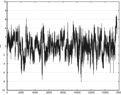
0 2000 4000 6000 8000 10000 12000 14000 16000 10
8 6 4 2 0 2 4 6 8 10
nT
Fig. 5. Experimental modulus residual (difference between the reconstructed modulus and the measured one) obtained when rotating the sensor in the earth magnetic field. In abscissae, the number of the measurement.
In order to appreciate the results, we have first to exam-ine the following question: suppose the algorithm has found the optimum solution, i.e. the right calibration parameters, what peak to peak residual will be seen on the modulus dif-ference? If the peak to peak value of the noiseνi on the
measurements Bi is small compared to the value ofb, the
residualr=Brec−bwill be:
r=Brec−b=
3
i=1
(Bi+νi)2−b∼ 3
i=1
Bi b ν
i (12)
(the noise onbis much smaller)
Considering νi as three identical centered white noises
(same varianceσ2
ν), the variance of the residual may be
writ-ten as the sum of the variances of the three distributions
νiBi/b:
σ2 r =
3
i=1
Bi
b
2 σ2
ν. (13)
Hence, the vector resolution being 1 nT/√Hz with a 1 Hz bandwidth (as discussed in Subsection 2.2), the RMS noise on the scalar residual will beσr ∼=1 nT. The peak to peak noise is six times this value:
(Brec−b)p−p∼=6 nT. (14)
Experimentally, the observed peak to peak value is close to 6 nT (see Fig. 5). Looking closer to Fig. 5, one can see in-deed that locally the peak to peak value is of the order of the calculated limit. Thus the parameter set obtained is not far from the optimum. However, a low frequency fluctuation re-mains on the scalar residual which reflects small fluctuations in the vector measurements. A tentative explanation of such variations is that bandwidth fluctuations affect the scalar he-lium pumped magnetometer so that transfer functions seen by the three modulations vary slightly with time. Further possible improvements can be imagined. First of all, those
bandwidth fluctuations could be reduced by working on the stability of the resonance excitation mechanism (laser or ra-dio frequency oscillator). The bandwidth itself could be en-larged (working on the electronics frequency together with a new operating point in terms of RF amplitude and light power) in such a way that the influence of the fluctuations at the modulation frequencies would be reduced. But the most efficient way of getting rid of this low frequency noise is to correct its effect by modeling the scalar bandwidth and then forcing the scalar residual to zero in order to estimate the scalar cutoff frequency.
The accuracy of the so obtained βi, α, θ, γ values has
been also estimated by drawing randomly 200 subsets of 1000 datab,h1,h2,h3quadruplets from the 16000 ones
available, and studying the dispersion of the corresponding 200 calibrations. Results are the following;
Departures from orthogonality are, in degrees:
α= −0.1479◦, θ=0.0015◦, γ =0.0026◦,
with an uncertainty of 4·10−4deg=7·10−6rad.
Modula-tion valuesβare of the order of 50 000 pT with an accuracy of .2 pT (compare with the 1.5·10−6rad and 7·10−5nT
val-ues of Subsection 3.5 for the case of synthetic data). These accuracies are close to the ones requested to obtain the Bi
components with six significant digits.
6.
Conclusion
In the introduction we presented the vector4Hepumped magnetometer as a possible candidate for an automatic abso-lute magnetic observatory. Results obtained up to now and presented here lead us to think that the corresponding re-quested performances—see Introduction—should likely be obtained. Efforts are still to be made, mainly to reduce the long bandwidth fluctuations which affect the scalar he-lium magnetometer. Tests of a possible compensation of these fluctuations (the best solution to mitigate them as said above) are currently performed, with encouraging results.
re-tained here appears efficient. Let us stress again that we solve the problem using a linear algorithm. This algorithm can be extended to the calibration of satellite magnetome-ters as the Ørsted one (made of three fluxgate sensors and one scalar RMN) (Olsenet al., 2000); apparently the linear-ity of the problem was not seen before. As already stressed, the data used in the calibration process allow an “internal” calibration: angles between the physical axes of the sensor are determined. Determining the exact orientation of these axes with respect to the geographical axes (OX-North, OY-East, OZ-downward vertical) should not be too difficult in a magnetic observatory where independent absolute mea-surements are available, but not trivial. Recall indeed that, contrarily to variometers operated in classical observatories, which measure only small relative variations of the field components, an absolute automatic magnetometer measures these full components, and consequently its axes must be known with a high accuracy. Of course, we have not ad-dressed here the problem of the stability of pillars.
Now, providing a new version of ASMO is not our only objective. The4Hevector magnetometer might also be
ad-vantageously used in space. Indeed, the resulting instru-ment has reasonable dimensions (size, weight and power consumption). Its main advantage is the replacement of the actual classical combination of a standard classical fluxgate vector magnetomer plus an absolute scalar magnetometer. The scalar and vector measurements are obtained continu-ously, simultaneously and at the same point, which might simplify the design of a satellite carrying this sensor, and the treatment of the resulting data. Thus, this vector helium pumped magnetometer seems very well suited for the needs of a satellite instrument.
Acknowledgments. First author was supported by CNES and CEA (Th`ese CTCI). Second author was partly supported by grant INTAS/CNES 97-1048.
Appendix A. Recovering
and
AWe consider the compositionCof the stretching matrix
=
The last step of the internal calibration problem consists in recovering anglesα,θ, γ and coefficientsλ11,λ22, λ33
from the (already known – see Subsection 3.4) entries of the matrixG−1 =(CC∗∗). The entries of the 3×3 matrix
So, after computing the entries of the matrix G−1, we straightforwardly get unique (positive) values of λ11, λ22, λ33and sinα. Taking into account thatα < π2 we find cosα
and then (after substitution and simplification) get the fol-lowing elementary system of equations:
⎧
are known. It has the explicit solution ⎧
Forθ, γ < π2 this provides an unique solution. The simple numerical algorithm for calibration is clear from above.
Appendix B. Case of a Few Bad Lines in the Data
The dataset is made of N vectors (bk,h1k, h2k, h3k), and
we may assume that m N indices k out of N
cali-958 O. GRAVRANDet al.: ON THE CALIBRATION OF A VECTORIAL4HePUMPED MAGNETOMETER
Then 0 < p < 1 forn +m N. Fix n and consider
l <
N n
calibrations corresponding to random subsets
{k1, . . .kn} ⊂ {1, . . .N}. Then (from the binomial
distri-bution) the probability P that there are at least twoproper
(i.e. free of error data) calibrations is given by
P =P(l,p)=1−(1−p)l−l·p(1−p)l−1.
Ifm N is small and N large enough, one can easily find the corresponding values fornandlensuring a proba-bility P statistically significant. Then in a statistical sense we will have at least two proper (and therefore close to each other, up to a given precision) calibrations. Taking into ac-count thatnon-proper(i.e. based on data including bad lines) calibrations will present strong deviations from each other and from the true calibration, we have only to find two close enough answers out ofl.
References
Alldredge, L. R., A proposed automatic standard magnetic observatory,J. Geophys. Res.,65, N11, 3777–3786, 1960.
Alldredge, L. R. and I. Saldukas, An automatic standard magnetic observa-tory,J. Geophys. Res.,69, N10, 1963–1970, 1964.
Colegrove, F. D. and L. D. Schearer, Optical pumping of helium in the3S1
metastable statePhysical Review,119, 680–690, 1961.
Guttin, C., J.-M. L´eger, and F. Stoeckel, Realization of an isotropic scalar magnetometer using optically pumped helium 4,Journal de Physique III,4, 655–659, 1993.
Merayo, M. G., P. Brauer, F. Primdhal, J. R. Petersen, and O. V. Nielsen, Scalar calibation of vector magnetometer,Meas. Sci. Technol.,11, 120– 132, 2000.
Nielsen, O. V., J. R. Petersen, F. Primdhal, P. Brauer, B. Hernando, A. Fern´andez, M. G. Merayo, and P. Ripka, Development, construction and analysis of the Orsted fluxgate magnetometer,Meas. Sci. Technol.,6, 1099–1115, 1995.
Olsen, N., L. Toffner-Clauden, T. Risbo, P. Brauer, J. Merayo, F. Primd-hal, and T. Sabaka, In-Flight calibration methods used for the Oersted mission, inESA SP on Space Magnetometer Calibration, 2000. Press, C., S. Teukolsky, W. Vetterling, and B. Flannery, Numerical
Recipes in C. Second edition, Cambridge University Press, Cambridge, 1996.
Rasson, J. L., Proceedings of the VIth Workshop on Geomagnetic Obser-vatory Instruments Data Acquisition and Processing, publication scien-tifique et technique n 003, Institut Royal M´et´eorologique de Belgique, Avenue Circulaire 3, B-1180 Bruxelles.
Trigg, D. F. and R. L. Coles, Intermagnet, technical reference manual, 1999.