M-Estimators of Roughness and Scale
for
G
A
0
-Modelled SAR Imagery
Oscar H. Bustos
Facultad de Matemática, Astronomía y Física, Universidad Nacional de Córdoba, Ciudad Universitaria, 5000 Córdoba, Argentina Email: [email protected]
María Magdalena Lucini
Facultad de Matemática, Astronomía y Física, Universidad Nacional de Córdoba, Ciudad Universitaria, 5000 Córdoba, Argentina Email: [email protected]
Alejandro C. Frery
Centro de Informática, Universidade Federal de Pernambuco, CP 7851, 50732-970 Recife - PE, Brasil Email: [email protected]
Received 31 July 2001 and in revised form 10 October 2001
TheG0
Adistribution is assumed as the universal model for multilook amplitude SAR imagery data under the multiplicative model. This distribution has two unknown parameters related to the roughness and the scale of the signal, that can be used in image analysis and processing. It can be seen that maximum likelihood and moment estimators for its parameters can be influenced by small percentages of “outliers”; hence, it is of outmost importance to find robust estimators for these parameters. One of the best-known classes of robust techniques is that of M-estimators, which are an extension of the maximum likelihood estimation method. In this work we derive the M-estimators for the parameters of theG0
Adistribution, and compare them with maximum likelihood estimators with a Monte-Carlo experience. It is checked that this robust technique is superior to the classical approach under the presence of corner reflectors, a common source of contamination in SAR images. Numerical issues are addressed, and a practical example is provided.
Keywords and phrases:inference, likelihood, M-estimators, Monte-Carlo method, multiplicative model, speckle, synthetic aper-ture radar, robustness.
1. INTRODUCTION
The statistical modeling of synthetic aperture radar (SAR) imagery has provided some of the best tools for the processing and understanding of this kind of data. Among the statistical approaches the most successful is the multiplicative model.
This model offers a set of distributions that, with a few parameters, are able to characterize most of SAR data. This model is presented, for instance, in [1], and extended in [2].
This extension is a general and tractable set of distribu-tions within the multiplicative model, used to describe every kind of SAR return. It was then called a universal model, and its properties are studied in [3, 4, 5].
In this paper, the problem of estimating the parameters of this extension, namely of theG0
Adistribution, is studied for the single look (the noisiest) situation. Two typical estima-tion situaestima-tions arise in image processing and analysis, namely large and small samples, being the latter considered in this work. The small samples problem arises in, for instance,
im-age filtering where with a few observations within a window a new value is computed.
Statistical inference with small samples is subjected to many problems, mainly bias, large variance, and sensitivity to deviations from the hypothesized model. This last issue is also a problem when dealing with large samples.
Robustness is a quite desirable property for estimators, since it allows their use even in situations where the quality of the input data is not perfect [6, 7, 8]. Most image processing and analysis procedures (filtering, classification, segmenta-tion, etc.) use spatial data. Even experienced users are unable to guarantee that all the input data are free of spurious values and/or structures.
Figure1: Man-made corner reflectors on a SAR image.
unreliable. Figure 1 shows man-made corner reflectors, the white spot regularly placed horizontally along the middle of the image, possibly buildings, on a SAR image where crops predominate.
This paper presents classical estimators, namely those based on sample moments and the maximum likelihood ones, and derives robust M-estimators for the single lookG0
Amodel. Once these estimators are derived, several situations are com-pared by means of a Monte-Carlo experience. These estima-tors are then applied to SAR imagery, and it is shown that the robust approach exhibits a good performance even in the presence of corner reflectors.
M-estimators have been mainly used for symmetric data, being [7, 8] two very relevant exceptions. In this application they are computed, implemented, and assessed for speckled imagery that, as will be seen in the next section, follow laws whose densities can be highly asymmetric. Since speckle noise also appears in ultrasound B-scan, sonar and laser images, the procedures here presented have potential application in all these techniques.
2. NOTATION AND MODEL DEFINITION
In the following,1Awill denote the indicator function of the setA, that is,
A(α, γ)distribution is characterized by the following probability density function:
fx, (α, γ)= −2αx
γ(1+(x2/γ))1−α1(0,+∞)(x), −α, γ, x >0. (2) Multilook, intensity, and complex versions of this distribution can be seen in [2]. The polarimetric (multivariate) extension of theG0distribution is presented in [9].
The parameterαin (2) describes the roughness of the target, being small values (sayα <−15) usually associated to homogeneous targets, like pasture, values ranging in the [−15,−5]interval usually observed in heterogeneous clutter, like forests, and big values (−5< α <0for instance) com-monly seen when extremely heterogeneous areas, as urban spots, are imaged. Theγparameter is related to the scale, in the sense that if ZA is aG0
A(α,1)-distributed random
vari-able thenZ= √γZobeys aG0
A(α, γ)law and, therefore, it is related to the brightness of the scene. Both parameters are es-sential when characterizing targets, and in image processing techniques involving statistical modeling.
the score function of theG0
A(α, γ)distribution is given by
sx, (α, γ)=
The cumulative distribution function of such random vari-able is given by
This will be used to compute an estimator based on order statistics. In [5] a relation between a more general version of theG0
A(α, γ)law and Snedekor’sFdistribution is shown to allow writing (5) as a function of the cumulative distribution function of the latter.
The moments of aG0
A(α, γ)distribution are given by
EXk=
This distribution can be derived as the square root of the ratio of two independent random variables: one obey-ing a unitary-mean exponential distribution (which conveys the speckle noise in one look) and one following a Γ(α, γ) distribution, related to the unobserved ground truth, the backscatter. Densities of theG0
A(α, γ)distribution are shown in Figure 2, for α ∈ {−1,−3,−9}and the scale parameter
Following Barndorff-Nielsen and Blæsild [10], it is in-teresting to see these densities as log probability functions, particularly because theG0
Alaw is closely related to the class of hyperbolic distributions [11]. Figure 3 shows the densities of the G0
0.0
Figure 2: Densities of the G0
A(α, γα) distribution, with α ∈
Figure3: Densities of theG0
A(−2.5,7.0686/π )(solid line) and the
N(1,4(1.1781−π /4)/π )(dashes) distributions in semilogarith-mic scale, with mean value in dash-dot.
chosen, using (6), so that these distributions have equal mean and variance. The different decays of their tails in the loga-rithmic plot are evident: the former behaves logaloga-rithmically, while the latter decays quadratically. This behavior ensures the ability of theG0
Adistribution to model data with extreme variability.
3. INFERENCE FOR THEG0
AMODEL
It can be seen that the maximum likelihood estimators ofα andγ based in X1, . . . , XN, represented here byαˆML,N and
ˆ
γML,N, respectively, are given by
ˆ that the half and first order moments estimators ofαandγ based onX1, . . . , XN, denoted here byαˆMOM,Nand byγˆMOM,N, respectively, are given by the solution of
m1/2,N=γˆMOM1/4 ,N
Moment estimation is extensively used in remote sens-ing applications [2], mainly because it is inexpensive from the computational point of view and analytically tractable in most situations. In the presence of corner reflectors, though, severe numerical instabilities were observed.
A comparison among different estimators for rough-ness parameter of theG0
Adistribution was performed in [4] through a Monte-Carlo experience. No contamination was considered, and the αˆML estimator was the best one in
al-most all cases with respect to the mean square error (mse) and the closeness to the true value (bias) criteria, assuming γis known. No analytical comparison is possible, due to the complexity of the estimators.
In previous works (see [12], for instance) it is shown that moment and maximum likelihood estimators have many op-timal properties when the observations, x1, . . . , xN are the outcome from independent, identically distributed random variables, with common density f (·, (α, γ)). Among these properties, maximum likelihood estimators are asymptoti-cally unbiased, that is, if X1, . . . , XN is a sequence of inde-pendent, identically distributed random variables with com-mon density f (·, (α, γ)) then, whenN → ∞, it holds that
ˆ
Since the routines that compute both ML- and M-estimators require initial guesses, the unstable (and, therefore, unacceptable) behavior of moment estimators demanded the use of another technique. A procedure based on analogy using order statistics and moments [13], defined in the following forα <−1, was used.
IfXisG0
A(α, γ)distributed the median of the scaled ran-dom variableY =X/E(X)can be computed using (5)
Q2= 2 √
π
α
1/2−1 Γ(−α)
Γ(−α−1/2). (11)
This scaled median does not depend onγ, soαˆcan be esti-mated using the sample medianq2(y), wherey =(xi/¯x)i, using standard numerical tools. An estimate of γ using the first-order moment can then be computed as
ˆ
γ=π4m12,N
Γ(−α)ˆ
Γ(−αˆ−1/2) 2
. (12)
This estimator ofαderived from (11) and the one computed forγthrough (12) will be calledmixed estimatorfor(α, γ), and denoted(αˆMIX,γˆMIX).
In the following, ML- and M-estimators will be assessed in two situations: the pure model, when no contamination is present, and cases where outliers simulating a corner reflector enter the data.
The contamination model here considered is defined as a sequence of independent, identically distributed ran-dom variables X1, . . . , XN with common distribution func-tionF (·, (α, γ), , z)given by
Fx, (α, γ), , z=(1−)Fx, (α, γ)+δz(x), (13)
where δz(x) = 1[z,+∞)(x), with za “very big” value with respect to most of the values typically assumed by a random variable with distributionG0
A(α, γ). Equation (13) describes a contamination that occurs at random with probability, that is, in average N out of N samples will be “very big” values (corner reflectors), while N−N samples will obey theG0
A(α, γ)distribution (the background). The flexibility of theG0
A(α, γ)distribution will allow the modeling of any kind of background, namely crops, forests, and urban areas. The contamination valuezwill be chosen as a factor of the mean value of the underlying distributionG0
A(α, γ). Other contamination hypothesis may include different distributions for the departure of the model, and/or spatial dependence among observations.
In order to quantitatively assess the sensitivity of ML-estimators in our case, using the strong law of large numbers on (8) and assumingγ=1, it is immediate that
lim
N→∞αˆML,N(z)= −
EF (·,(α,γ),ε,z)ln1+X2
−1
= − 1
εln(1+z2)−(1−ε)(1/α).
(14)
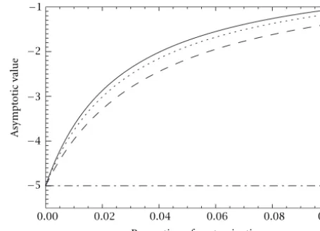
Figure 4 shows, for α = −5, this limit as a function of ε, the proportion of outliers in the sample, for several values of
0.00
−5
−4
−3
−2
−1
0.02 0.04 0.06 0.08 0.10
Proportion of contamination
A
sy
m
pt
otic
value
Figure4: Asymptotic value ofαˆML, under the contaminated model
withα= −5, as a function of the proportion of contamination
and outlier values−45(solid line),−30(dots), and−15(dashes).
the outlier z. Three values ofzare shown forε∈[0,0.1]. It can be seen that a sample that suffers from a small con-tamination of ε =0.02leads to the wrong conclusion that extremely heterogeneous targets are under observation, since the estimated value will be around−3whilst the true value is−5(corresponding to an heterogeneous target). The big-ger the contamination the worse this behavior. This influence on the ML-estimator is noticed regardless the value of zin the chosen range. This result justifies a careful analysis of the performance of estimators for a single representative value of the contaminationz, and for several values ofε, as presented in Section 5.
4. M-ESTIMATORS
These estimators offer a useful alternative when small propor-tions of values may be far from the bulk of data. A good survey on these estimators and their use in practical situations can be seen in [7]. The difficulty in our case arises due to the fact that the underlying distribution is asymmetric. Inspired in the work by Marazzi and Ruffieux [8], that robustified maxi-mum likelihood estimators for the parameters of the gamma distribution with success, we will compute M-estimators for the parameters of theG0
A(α, γ)distribution.
One has to devise ways to prevent a large influence of outliers in the likelihood equations. M-estimators propose the use of ψfunctions that truncate the score of influential observations in the likelihood equations.
Letb1andb2be two real positive numbers. We will call M-estimators of parametersα andγ based on the sample X1, . . . , XN, the statisticsαˆM,N, andγˆM,Nsuch that
N
k=1
ψb1
s1Xk,αˆM,N,γˆM,N−c1αˆM,N,γˆM,N, b1=0,
N
k=1
ψb2(s2(Xk,
ˆ
αM,N,γˆM,N−c2αˆM,N,γˆM,N, b2=0,
wheres1ands2are given in (4), andψb1andψb2are
ψbi(x)=
−bi ifx≤bi,
x if −bi< x < bi,
bi ifx≥bi,
(16)
withx∈ Randi=1,2. Note that making these functions the identity and c1 = c2 ≡0, equations (15) reduce to the familiar system of likelihood equations. Figure 5 illustrates the ψ6(x) function, where its effect on the data becomes clear: it truncates the score of those values above and below its threshold. In this manner, this function prevents abnormal (too small and too big) data having excessive influence on the estimates.
The functionsci:Θ×(0,+∞)→Rin (15) are defined in such way that(αˆM,N,γˆM,N)Nis a sequence of asymptotically unbiased estimators of(α, γ), that is,
ψb1
s1x, (α, γ)−c1α, γ, b1fx, (α, γ)dx=0,
ψb2
s2(x, (α, γ)
−c2
α, γ, b2
fx, (α, γ)dx=0, (17) for any(α, γ)∈Θ,b1>0andb2>0. The computation of these functions is presented in Appendices A and B.
−10 −5 0 5 10
10
5
−5
−10
Figure5: Theψ6function used to define M-estimators.
The valuesb1andb2, called “tuning parameters” are cho-sen in such a way that the efficiency of the M-estimators is not unacceptably poor with respect to the maximum likelihood ones. Thus, we will chooseb1andb2such that
VαˆML
VαˆM e1,
VγˆML
VγˆM e2, (18)
whereVdenotes variance, with0.9≤ei≤0.975for exam-ple. This restriction imposes that the variance of the robust estimators will not surpass those of the maximum likelihood ones in more than a certain factor. The computation of these parameters is done in Appendix C.
In order to assess the finite sample behavior of the pro-posed estimators consider the situation whereNobservations from independent identically distributedG0
A(α, γ)random
−8
−6
−4
−2 0
5 10 15
Contamination Value
ML
an
d
M
E
st
im
ators
Figure6: Maximum likelihood (continuous line) and M-(dotted line) estimators for the estimation of αand γin a sample with
N=77pure observations andM=4contaminated values.
variables are contaminated byLobservations taking the value z. The contaminated samplez=(z1, . . . , zN, z, . . . , z ), where
the brackets denote theN+Loutliers, will be used to esti-mate αandγ. Depending on the true parameters, on the contamination (the valuez and the number of outliersL) and on the sample sizeN, it is expected that any non-robust estimator will be mislead by the departure from the hypoth-esized model. Figure 6 shows the maximum likelihood and M-estimators for the situation whereN=77pure observa-tions andL=4equal contaminated values are used. It can be seen that the former suffers from both the departure from the true model and from numerical instabilities (the peak around the value10). It is noticeable that the robust estima-tor remains closer to the true value (the dash-dot line) than the other in the presence of contamination. The bigger the value of the contamination the further maximum likelihood will go from the true value, while the M-estimator will render the same estimate. The same behavior was observed for the estimators of γ. The values employed forN,L,αandzare representative of the kind of problem at hand: filtering im-ages over a heterogeneous area (α= −3) with9×9windows (N+L=81) where some observations (L=4) are due to a corner reflector (zvarying and taking large values).
5. RESULTS
A Monte-Carlo experience was performed to compare maxi-mum likelihood (ML) and M-estimators (M), since analytical comparisons are unfeasible.G0
value1, that is,γ=γα=4(Γ(−α)/Γ(−α−1/2))2/π. We studied four models that will be identified as Models 1, 2, 3, and 4: Model 1 (the “ pure” model) consisting of sam-ples of theF (·, (α, γα))distribution; Model 2 consisting of samples taken from theF (·, (α, γα), , z)distribution with
=0.01andz=15, Model 3 is a collection of samples ob-tained from theF (·, (α, γα), , z)distribution with=0.05 andz=15, while Model 4 is a collection of samples obtained from theF (·, (α, γα), , z)distribution with = 0.10and
z = 15. In this manner, the pure situation and three levels of contamination are examined. The contamination valuez is held fixed, as discussed in Section 3, as fifteen times the expected value of the underlying model which is big enough to describe corner reflectors.
In each of these models we deal with three situations, namely with: Situation 1 (α= −1.0), Situation 2 (α= −3), and Situation 3 (α= −6). These situations cover representa-tive targets in practice: extreme heterogeneity, heterogeneity and homogeneity.
In order to determine the number of replications an em-pirical precision criterion was used. One hundred replications (1≤r ≤ R =100) with samples of sizeN = 9×9=81 were performed. One estimator forαis computed for each replication r, say α(r )ˆ . The final number of replications R =R+ , ≥ 1integer, is the smallest number of sam-ples that allows forming an asymptotic confidence interval at the 95% level on the mean of the R estimators, that is, 2×1.96sR/
√
R <0.5wheresRis the standard deviation of the sample{α(ˆ 1), . . . ,α(R)ˆ }. This is computed for every es-timator forαand every estimator forγ in every model and every situation. The biggest number of replications R (the worst case) is then used. This procedure led toR =101in every model and every situation.
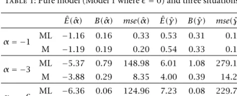
The following tables show the results obtained in this study for each situation: for every model the sample mean of the estimator over theRreplicationsE(ζ)ˆ =R−1R
r=1ζ(r ), the mean square errormse=E(ζˆ −θ)2=V (ζ)ˆ +(E(ζ)ˆ −θ)2, and the absolute relative biasB(ζ)=θ−1|E(ζ)ˆ −θ|, where
θ is the true value of the parameter andζis the estimator under study.
In all the tables it can be seen that M-estimators are almost as good as ML-estimators when there is no contamination, while in the presence of outliers M-estimators exhibit smaller absolute relative bias and smaller mean squared error. Asαis smaller (the observed region is more homogeneous),
estima-Table1: Pure model (Model 1 where=0) and three situations. ˆ
E(α)ˆ B(α)ˆ mse(α)ˆ E(ˆγ)ˆ B(γ)ˆ mse(γ)ˆ
α= −1 ML −1.16 0.16 0.33 0.53 0.31 0.16
M −1.19 0.19 0.20 0.54 0.33 0.11
α= −3 ML −5.37 0.79 148.98 6.01 1.08 279.11 M −3.88 0.29 8.35 4.00 0.39 14.25
α= −6 ML −6.36 0.06 124.96 7.23 0.08 229.72 M −6.25 0.04 69.13 7.08 0.06 122.36
Table2: Model 2 (=0.01) and three situations.
ˆ
E(α)ˆ B(α)ˆ mse(α)ˆ E(ˆγ)ˆ B(γ)ˆ mse(γ)ˆ
α= −1 ML −0.97 0.03 0.22 0.41 0.01 0.08
M −1.01 0.01 0.15 0.49 0.20 0.08
α= −3 ML −2.96 0.01 25.07 2.72 0.05 46.06
M −3.10 0.03 3.28 3.17 0.10 5.65
α= −6 ML −2.76 0.54 16.10 2.89 0.57 22.32
M −4.28 0.28 7.41 4.77 0.29 9.43
Table3: Model 3 (=0.05) and three situations.
ˆ
E(α)ˆ B(α)ˆ mse(α)ˆ E(ˆγ)ˆ B(γ)ˆ mse(γ)ˆ
α= −1 ML −0.68 0.32 0.12 0.27 0.33 0.03
M −0.86 0.14 0.12 0.39 0.04 0.08
α= −3 ML −0.89 0.70 4.45 0.70 0.76 4.87
M −2.01 0.33 1.46 2.13 0.26 1.60
α= −6 ML −0.93 0.84 25.51 0.81 0.88 34.84
M −2.51 0.58 12.67 2.96 0.56 15.31
Table4: Model 4 (=0.10) and three situations. ˆ
E(α)ˆ B(α)ˆ mse(α)ˆ E(ˆγ)ˆ B(γ)ˆ mse(γ)ˆ
α= −1 ML −0.61 0.39 0.16 0.25 0.38 0.08
M −0.71 0.29 0.13 0.33 0.18 0.04
α= −3 ML −0.69 0.77 5.34 0.52 0.82 5.60
M −1.39 0.54 2.80 1.56 0.46 2.24
α= −6 ML −0.71 0.88 27.88 0.58 0.91 37.08
M −1.70 0.72 18.85 2.15 0.68 21.20
tion becomes less reliable. This is probably due to the shape of the likelihood function, that becomes flat and, therefore, is hard to find its maximum location. The bigger the proportion of contamination the worse the behavior of both estimators, but M-estimators remain consistently closer to the true value than ML-estimators, as expected.
As an application, the image shown in Figure 7 is ana-lyzed. Windows of size9×9are used to estimate the back-ground parameters over a trajectory that spans from the up-per left corner to the lower right corner. This trajectory passes through the three corner reflectors of the image, which are clearly seen as white spots.
posi-Figure7: Image with three corner reflectors over a heterogeneous background.
−10
−8
−6
−4
−2 0
10 20 30 40
Position
Estimat
ors
Figure8: Estimatedαusing9×9windows: ML (solid line) and M-(dashes) estimators.
tions (the gaps in the solid line). Similar results were observed estimating the scale parameterγ.
6. CONCLUSIONS AND FUTURE WORK
There are numerical problems with the computation of these estimators for certain parameters. For small samples there is often no solution, being this situation more critical for small values ofα, that is, for homogeneous areas. This issue will be further investigated in future works.
As it can be seen from the tables, in the pure model (Model 1), the behavior of the robust estimators is as good as the maximum likelihood ones, as it is expected. In the
contaminated situations (Models 2 and 3), we can see that estimation by moments or maximum likelihood methods is poor.
It is relevant to notice that under a very small contami-nation or a very small deviation from the model the behavior of the classical estimators is not reliable.
This work will continue computing the M-estimators for the multilook case, that is, for the n >1situation and for polarimetric (multivariate) data. An alternative approach us-ing alpha-stable distributions [14] is also possible, but at the expense of loosing the interpretability of the parameters that stem from the multiplicative model.
APPENDICES
A. COMPUTATION OFc1
Let α < 0. The problem consists of findingc1(α,1) that satisfiesI1(α, c1, b)=0, whereI1(α, c, b)=
∞
0 ψb((1/α)+ ln(1+u)−c)((−α)/(1+u)1−α)duis the equation that has to be solved in order to define the M-estimators for theG0 A distribution (equations (15)).
Lemma A.1. Letα <0, then
(1)Ifexp(2αb) > bα+1then there existsc0, with−b+
α−1< c
0< b+α−1that satisfiesI1(α, c0, b)=0. In this case
c0isαc0=exp(αb+αc0−1).
(2)Ifexp(2αb) < bα+1then there existsc0, withc0≥
b+α−1that satisfiesI
1(α, c0, b)=0, and it is given byc0=
α−1(ln(−α)+ln(b)−ln(e−αb−eαb)+1).
Proof. The function G(c) = I1(α, c, b) is a continuous monotone decreasing function, then
lim
c→−∞G(c)=b, clim→∞G(c)= −b. (A.1)
Therefore, there exitsc0that satisfiesG(c0)=I1(α, c0, b)= 0. Denoting A= A(α, c) = exp(−b−(1/α)+c)−1and B=B(α, c)=exp(b−α−1+c)−1, thenA < Band one can write
ψb
1
α+ln(1+u)−c
=
−b ifu < A,
1
α+ln(1+u)−c ifA < u < B,
b ifu > B.
(A.2)
Ifc <−b+α−1, thenB <0, and thenI
1(α, c, b)=b. So, there is noc0<−b+α−1satisfyingI1(α, c0, b)=0. If
−b+α−1≤c < b+α−1, thenA <0< Band, therefore,
I1(α, c, b)=exp
(αb+αc−1)
α −c. (A.3)
AsI1(α,−b+α−1, b)=b >0, thenc0>−b+α−1, and
I1
α,−b+ 1 α, b
= 1
α
If I1(α,−b+(1/α), b) < 0, then there exits −b+α−1 <
B. COMPUTATION OFc2
Let α < 0 andγ > 0. As for the computation of c1, the problem of finding the functionc2consists of findingc2=
c2(α, γ, b2)that satisfies than in the computation of c1 due to the presence of the parameterγ.
Lemma B.1. Letα <0andγ >0. In order to find the function c2that satisfies(B.1)one has to consider the following cases:
(1) if1−α−2γb2>0then by the solutionc2that makes equation (B.6) zero.
I2(α, γ, c, b2)= −((−γb2−α−c)/(1−α))1−α−c. Taking
c = −α−γb2, thenI2(α, γ,−α−γb2, b2)= α+γb2. As
I2(α, γ,−α−γb2, b2) < 0if γb2 < −α, one can say that
c2satisfying equation (B.1) is given by the solution ofc2=
−((−γb2−α−c2)/(1−α))1−α.
But, ifγb2≥ −α, one can take−γb2−α < c≤γb2− 1. In this case one has that I2(α, γ, c, b2) = −c, therefore
I2(α, γ, γb2−1, b2)=1−γb2. Thus, if1< γb2one can say that the solution of equation (B.1) isc2=0.
Ifγb2≤1, then one takesc > γb2−1, leading to
I2
α, γ, c, b2
=
γb
2−α−c 1−α
1−α
−γb2. (B.8)
Hence,c2=γb2−α−(γb2)1/(1−α)(1−α)is the solution of (B.1).
C. COMPUTATION OF TUNING PARAMETERS
The definition of efficient M-estimators requires finding tun-ing parametersb1andb2ensuring that the relative asymp-totic variance (with respect to the variance of maximum likelihood estimators) satisfies V (αˆML)/V (αˆM) e1 and
V (γˆML)/V (γˆM) e2 with, for instance,0.9≤ ei ≤ 0.975.
V (αˆML), V (γˆML) and V (αˆM), V (γˆM) are the diagonal
el-ements of the asymptotic covariance matrix of the ML-and M-estimators of parameters αandγ, here denoted by V ((α,ˆ γ)ˆ ML)andV ((α,ˆ γ)ˆ M), respectively.
C.1. Computation ofV ((α, γ)ML)
We denote
V(α, γ)ML=Ms, F (α, γ)−1J(α, γ)Ms, F (α, γ)−T,
(C.1) where F (α, γ) is the cumulative distribution function of a random variable having G0A(α, γ,1) distribution, s =
s(x, (α, γ))is the vector of score functions,
J(α, γ)=
sx, (α, γ)sx, (α, γ)TdFx, (α, γ) (C.2)
is the Fisher information matrix, and
Ms, F (α, γ)= − ∂ ∂(α, γ)s
x, (α, γ)dFx, (α, γ).
(C.3) It can be seen that
J(α, γ)=
α−2 γ(1−α)−1 γ(1−α)−1 −α(2−α)γ2−1
, (C.4)
and that
Ms, F (α, γ)=J(α, γ)
=
α−2 γ(1−α)−1 γ(1−α)−1 −α(2−α)γ2−1
.
(C.5)
Therefore, replacing matrix (C.4) and the inverse of ma-trix (C.5) in equation (C.1), we have
V(α, γ)ML
=
α2(1−α)2 γα(1−α)(2−α) γα(1−α)(2−α) −α−1γ2(1−α)2(2−α)
.
(C.6)
C.2. Computation ofV ((α, γ)M)
We define
V(α, γ)M=MΨ, F (α, γ)−1Q(α, γ)MΨ, F (α, γ)−T,
(C.7) where
Ψ=Ψx;(α, γ)= ψb1
s1(x;(α, γ)−c1α, γ, b1)
ψb2s2(x;(α, γ)−c2α, γ, b2
,
MΨ, F (α, γ)= −∂α∂ Ψx, (α, γ)dFx, (α, γ),
Q(α, γ)=
Ψx, (α, γ)Ψx, (α, γ)TdFx, (α, γ).
(C.8) The matricesMandQare computed taking into account all the cases that define the functionsci,i=1,2, and solving explicitly the integrals.
ACKNOWLEDGEMENT
The authors are grateful to Conicor, SeCyT, CNPq, and Vitae for the partial support of this research.
REFERENCES
[1] C. Oliver and S. Quegan, Understanding Synthetic Aperture Radar Images, Artech House, Boston, 1998.
[2] A. C. Frery, H.-J. Müller, C. C. F. Yanasse, and S. J. S. Sant’Anna, “A model for extremely heterogeneous clutter,”IEEE Transac-tions on Geoscience and Remote Sensing, vol. 35, pp. 648–659, 1997.
[3] J. Jacobo-Berlles, M. Mejail, and A. C. Frery, “The GA0 distri-bution as the true model for SAR images,” inSimpósio Brasileiro de Computação Gráfica e Processamento de Imagens, SBC, IEEE, Campinas, SP, Brazil, 1999.
[4] M. Mejail, J. Jacobo-Berlles, A. C. Frery, and O. H. Bustos, “Parametric roughness estimation in amplitude SAR images under the multiplicative model,”Revista de Teledetección, vol. 13, pp. 37–49, 2000.
[5] M. E. Mejail, A. C. Frery, J. Jacobo-Berlles, and O. H. Bus-tos, “Approximation of distributions for SAR images: Pro-posal, evaluation and practical consequences,”Latin American Applied Research, vol. 31, pp. 83–92, 2001.
[6] O. H. Bustos, “Robust statistics in SAR image processing,” inProceedings of the First Latino-American Seminar on Radar Remote Sensing: Image Processing Techniques, pp. 81–89, ESA, Paris, 1996.
[7] F. R. Hampel, E. M. Ronchetti, P. J. Rousseeuw, and W. A. Stahel, Robust Statistics: The Approach Based on Influence Functions, Wiley, New York, 1986.
and Computer Intensive Methods, R. Helmut, Ed., vol. 109 of Lecture Notes in Statistics, Springer-Verlag, Berlin, 1996. [9] A. C. Frery, A. H. Correia, C. D. Rennó, C. C. Freitas, J.
Jacobo-Berlles, M. E. Mejail, and K. L. P. Vasconcellos, “Models for synthetic aperture radar image analysis,”Resenhas (IME-USP), vol. 4, no. 1, pp. 45–77, 1999.
[10] O. E. Barndorff-Nielsen and P. Blæsild, “Hyperbolic distribu-tions and ramificadistribu-tions: Contribudistribu-tions to theory and applica-tions,” inStatistical distributions in scientific work, C. Taillie and B. A. Baldessari, Eds., pp. 19–44, Reidel, Dordrecht, 1981. [11] A. C. Frery, C. C. F. Yanasse, and S. J. S. Sant’Anna, “Alter-native distributions for the multiplicative model in SAR im-ages,” inQuantitative remote sensing for science and applications, IGARSS’95 Proc., pp. 169–171, IEEE, Florence, July 1995. [12] P. K. Sen and J. M. Singer, Large Sample Methods in Statistics:
An Introduction with Applications, Chapman and Hall, London, 1993.
[13] C. F. Manski, Analog Estimation Methods in Economet-rics, vol. 39 of Monographs on Statistics and Applied Prob-ability, Chapman & Hall, New York, 1988, available at http://elsa.berkeley.edu/books/analog.html.
[14] C. L. Nikias and M. Shao, Signal Processing with Alpha-Stable Distributions and Applications, Wiley, New York, 1995.
Oscar H. Bustosreceived the B.S. degree in Mathematics from the Universidad Na-cional de Córdoba, Argentina, in 1970 and the Ph.D. in Mathematics from the Univer-sidad Nacional de San Luis, Argentina, in 1978. He is Professor at the Universidad Na-cional de Córdoba (Mathematics, Physics and Astronomy Institute) and his research areas include mathematical and statistical
models for image processing, robustness in statistics and stochastic simulation.
María Magdalena Lucinireceived the B.S. degree in Mathematics from the Univer-sidad Nacional de Córdoba (Mathematics, Physics and Astronomy Institute) in 1996. She is currently pursuing the Ph.D program in Mathematics at the same university. Her research interests are statistical signal pro-cessing with emphasis in robust statistics, estimation and filtering theory and
appli-cations in signal and image processing for imaging under severe noise.
Alejandro C. Freryreceived the degree in Electronic Engineering from the Universi-dad de Mendoza, Argentina, in 1987. His MSc degree was in Applied Mathematics (Statistics) from the Instituto de Matemática Pura e Aplicada (IMPA, Rio de Janeiro, Brazil, 1990) and his Ph.D. was in Applied Computing from the Instituto Nacional de Pesquisas Espaciais (INPE, São José dos