R E S E A R C H
Open Access
Distributed Gram-Schmidt
orthogonalization with simultaneous elements
refinement
Ondrej Sluˇciak
1, Hana Straková
2, Markus Rupp
1*and Wilfried Gansterer
2Abstract
We present a novel distributed QR factorization algorithm for orthogonalizing a set of vectors in a decentralized wireless sensor network. The algorithm is based on the classical Gram-Schmidt orthogonalization with all projections and inner products reformulated in a recursive manner. In contrast to existing distributed orthogonalization
algorithms, all elements of the resulting matricesQandRare computed simultaneously and refined iteratively after each transmission. Thus, the algorithm allows a trade-off between run time and accuracy. Moreover, the number of transmitted messages is considerably smaller in comparison to state-of-the-art algorithms. We thoroughly study its numerical properties and performance from various aspects. We also investigate the algorithm’s robustness to link failures and provide a comparison with existing distributed QR factorization algorithms in terms of communication cost and memory requirements.
Keywords: Distributed processing, Gram-Schmidt orthogonalization, QR factorization
1 Introduction
Orthogonalizing a set of vectors is a well-known prob-lem in linear algebra. Representing the set of vectors by a matrix A ∈ Rn×m, with n ≥ m, several orthogo-nalization methods are possible. One example is the so-calledreduced QR factorization(matrix decomposition),
A = QR, with a matrixQ ∈ Rn×m having orthonor-mal columns, and an upper triangular matrixR∈Rm×m
containing the coefficients of the basis transformation [1]. In the signal processing area, QR factorization is used widely in many applications, e. g., when solving linear least squares problems or decorrelation [2–4]. In adap-tive filtering, a decorrelation method is typically used as a pre-step for increasing the learning rate of the adaptive algorithm [5], ([6], p. 351), ([7], p. 700).
From an algorithmic point of view, there are many methods for computing QR factorization with different numerical properties. A standard approach is the
Gram-Schmidt orthogonalization algorithm, which computes a
set of orthonormal vectors spanning the same space as the
*Correspondence: [email protected]
1TU Wien, Institute of Telecommunications, Gusshausstrasse 25/E389, 1040 Vienna, Austria
Full list of author information is available at the end of the article
given set of vectors. Other methods include Householder reflections or Givens rotations, which are not considered in this paper.
Optimization of QR factorization algorithms for a spe-cific target hardware has been addressed in the literature several times (e.g., [8, 9]). Parallel algorithms for com-puting QR factorization, which are applicable for reliable systems with fixed, regular, and globally known topology, have been investigated extensively (e.g., [10–13]).
Besides parallel algorithms, there are two other poten-tial approaches for computation across a distributed net-work. In the standard—centralized—approach, the data are collected from all nodes and the computation is per-formed at a fusion center. Another approach is to consider distributed algorithms for fully decentralized networks without any fusion center where all nodes have the same functionality and each of them communicates only with its neighbors. Such an approach is typical for sensor-actuator networks or autonomous swarms of robotic net-works [14]. Nevertheless, the investigation ofdistributed
QR factorization algorithms designed for loosely cou-pled distributed systems with independently operating distributed memory nodes and with possibly unreliable communication links has only started recently [3, 15, 16].
In the following, we focus on algorithms for such decen-tralized networks.
1.1 Motivation
The main goal of this paper is to present a novel dis-tributed QR factorization algorithm—DS-CGS—which is based on the classical Gram-Schmidt orthogonalization. The algorithm does not require any fusion center and assumes only local communication between neighboring nodes without any global knowledge about the topol-ogy. In contrast to existing distributed approaches, the DS-CGS algorithm computes the approximations of all elements of the new orthonormal basis simultaneously
and as the algorithm proceeds, the values at all nodes are refined iteratively, approximating the exact values of
QandR. Therefore, it can deliver an estimate of the full matrix resultat any moment of the computation. As we will show, this approach is, among others, superior to existing methods in terms of the number of transmitted messages in the network.
In Section 2, we briefly recall the concept of a consensus algorithm which we use later in the distributed orthogo-nalization algorithm. In Section 3, we review the basics of the QR decomposition and existing distributed methods. In Section 4, we describe the proposed distributed Gram-Schmidt orthogonalization algorithm with simultaneous refinements of all elements (DS-CGS). We experimentally compare DS-CGS with other distributed approaches in Section 5 where we also investigate the properties of DS-CGS from many different viewpoints. Section 6 concludes the paper.
1.2 Notation and terminology
In what follows, we usekas the node index,Nk denotes the set of neighbors of nodek,N denotes the (known) number of nodes in the network,E the set of edges (links) of the network,dkthekth node degree (dk = |Nk|),d¯ the average node degree of the network, andta discrete time (iteration) index.
We will describe the behavior of the distributed algo-rithm from a network (global) point of view with the corresponding vector/matrix notation. For example, the (column) vector of all ones denoted by1, corresponds to all nodes having value 1. In general, we denote the num-ber of rows of a matrix bynand the number of columns bym. Element-wise division of two vectors is denoted as
z= xy ≡ xi
yi,∀i, element-wise multiplication of two vectors
asz=x◦y≡xiyi,∀iand of two matrices asZ=X◦Y. The operationXYis defined as follows: Having two matrices
X= (x1,x2,. . .,xm)andY= (y1,y2,. . .,ym), the
result-creating a big matrix containing combinations of column
vectors:Z∈Rn×m22−m. This later corresponds in our algo-rithm to the off-diagonal elements of the matrixR. Also note that all variables with the “hat” symbol, e.g.,uˆ(t) rep-resent variables that are computed locally at nodes, while variables with the “tilde” symbol, e.g.,u˜(t), are updated based on the information from neighbors.
2 Average consensus algorithm
We model a wireless sensor network (WSN) by syn-chronously working nodes which broadcast their data into their neighborhood within a radiusρ(so-called geometric topology). The WSN is considered to be static, connected, and with error-free transmissions (except for Section 5.4 ahead). Although the practicality of synchronicity can be argued [17, 18], we note that it is not an unrealizable assumption [19].
In the following, we briefly review the classical con-sensus algorithm for computing the average of values distributed in a network. Note that the algorithm can be easily adapted to computing asumby multiplying the final average value (arithmetic mean) by the total number of nodesN.
The distributed average consensus algorithm computes an estimate of the globalaverageof distributed initial data
x(0)at each nodekof a WSN. In every iterationt, each node updates its estimate using the weighted data received from its neighbors, i.e.,
xk(t)=[W]kkxk(t−1)+
k∈Nk
[W]kkxk(t−1)
or from a global (network) point of view
x(t)=Wx(t−1). (1)
The selection of theweight matrixW, representing the connections in a strongly connected network, crucially influences the convergence of the average consensus algo-rithm [20–22]. The main condition for the algoalgo-rithm to converge is that the largest eigenvalue ofWis equal to 1, i.e.,λmax=1, with multiplicity one, and that each row of Wsums up to 1. It can then be directly shown [20] that the valuexk(t)at each node converges to a common global value, e.g., average of the initial values.
If not stated otherwise, we use the so-called Metropolis weights [22] for matrixW, i.e.,
[W]ij=
3 QR factorization
As mentioned in Section 1, there exist many algorithms for computing the QR factorization with different proper-ties [1, 23]. In this paper we utilize the QR decomposition based on theclassical Gram-Schmidt orthogonalization method (in2space).
3.1 Centralized classical Gram-Schmidt orthogonalization Given matrixA= (a1,a2,. . .,am)∈ Rn×m,n≥m, clas-sical Gram-Schmidt orthogonalization (CGS) computes a matrixQ ∈ Rn×m with orthonormal columns and an
It is known that the algorithm is numerically sensitive depending on the singular values (condition number) of matrix Aas well as it can produce vectors qi far from orthogonal when the matrixAis close to being rank defi-cient even in a floating-point precision [23]. Numerical stability can be improved by other methods, e.g., modified Gram-Schmidt method, Householder transformations, or Givens rotations [1, 23].
3.2 Existing distributed methods
Assuming that each nodekstores its local valuesu2k and
qkak, it is then straightforward to redefine the CGS in a distributed way, suitable for a WSN, by following the def-inition of the2norm, i.e.,u22 = u21+u22+ · · · +u2n
(cf. (4)), and inner products, q,a =q1a1+q2a2+ · · · + qnan (cf. (5)). The summations can then be computed using any distributed aggregation algorithm, e.g., average consensus [20]1(see Section 2), and asynchronous gossip-ing algorithms [24], usgossip-ing only communication with the neighbors.
Nevertheless, to our knowledge, all existing distributed algorithms for orthogonalizing a set of vectors are based on the gossip-basedpush-sum algorithm[16, 24]. Specif-ically in [3], authors used a distributed CGS based on
gossiping for solving a distributed least squares prob-lem and in [15], a gossip-based distributed algorithm
formodifiedGram-Schmidt orthogonalization (MGS) was
designed and analyzed. The authors also provided a quan-titative comparison to existing parallel algorithms for QR factorization. A slight modification of the latter algorithm was introduced in [25], which we use for comparison in this paper. We denote the two Gossip-based distributed Gram-Schmidt orthogonalization algorithms as G-CGS [3] and G-MGS [25], respectively.
Since the classical Gram-Schmidt orthogonalization computes each column of the matrixQfrom the previ-ous column recursively, i.e., to know vectorq2, we need to compute the norm ofu2which depends on vectorq1, the existing distributed algorithms always need to wait for convergence of one column before proceeding with the next column. This may be a big disadvantage in WSNs as it requires a lot of transmissions. Also, if the algorithm fails at some moment, e.g., due to transmission errors, the matricesQandRare incomplete and unusable for further application.
In contrast, the distributed algorithm proposed in this paper overcomes these disadvantages and computes approximations of all elements of the matrices Q and
Rsimultaneously. All the norms and inner products are refined iteratively which leads to a significant decrease of transmitted messages, and also the algorithm brings an intermediate approximation of the whole matricesQand
Rat any time instance.
4 Distributed classical Gram-Schmidt with simultaneous elements refinement
As mentioned in Section 3.2, the Gram-Schmidt orthog-onalization method can be computed in a distributed way using any distributed aggregation algorithm. We refer to CGS based on the average consensus (see Section 2) as AC-CGS. AC-CGS as well as G-CGS [3] and G-MGS [25] have the following substantial drawback.
In all Gram-Schmidt orthogonalization methods, the computation of the norms ui and the inner prod-ucts qj,ai, qj,qj, occurring in the matrices Qand R, depends on the norms and inner products computed from the previous columns of the input matrixA. Therefore, each nodekmustwaituntil the estimates of the previous norms uj (j < i) have achieved an acceptable accu-racy before processing the next normui(a “cascading” approach; see [15]). The same holds also for computing the inner products. We here present a novel approach overcoming this drawback.
Rewriting Eqs. (4) and (5) by a recursion, we obtain
whereu˜i(t)is the approximation of 1/Nui221at timet
Similarly to the state-of-the-art methods (see Section 3.2), we further assume that the matrices
A ∈ Rn×m andQ ∈ Rn×m are distributed over the network row-wise, meaning that each node stores at least one row of the matrixAand corresponding rows of the matrix Qand each node stores the whole matrix R. In casen > N, more rows must be stored at the node and each node must sum the data locally before broadcasting to neighbors. Obviously, the data distribution over the network influences the speed of convergence of the algo-rithm, as can be seen also in the simulations ahead (see Section 5).
From aglobal(network) point of view, the algorithm is defined in Algorithm 1.
Proof of convergence of DS-CGS.For the first column,
vector i = 1, uˆ1(t) = a1, and thus the convergence results of the average consensus, see Section 2, apply, i.e., ast → ∞, the nodes will monotonically reach the common values, i.e., u˜1(t) = 1/Na1221and thus also,
Furthermore, for all columns i > 1, all the ele-ments depend only on the first column (i = 1), e.g.,
to u2 (Eq. (5)) and similarly will do all norms and inner products (Eqs. (4) and (5)) of matrixQandR.
Intuitively, we can see that as u˜1(t) converges to its steady state, all other variables converge, with some “delay,” to their steady states as well. We may say that as the first column converges, it “drags” other elements to their
Algorithm 1: DISTRIBUTEDGRAM-SCHMIDT ORTHOGONALIZ ATION WITHSIMULTANEOUS REFINEMEN T(DS–CGS)
• Input matrixA=(a1,a2,. . .,am)∈Rn×mwith n≥mis distributed row-wise acrossN nodes. If n>N, some nodes store more than one row. Each node computes the rows ofQcorresponding to the stored rows ofAand an estimate of the whole matrix R. indices:k= 1, 2,. . .,N(nodes);i=1, 2,. . .,m
(a) Compute locally at each nodek
pi(t)=ij=−11
Note that instead of knowing the number of nodes N and using it as a normalization con-stant, we could transmit an additional weight vector ω(t) ∈ RN×1, i.e., (0)(t) = ω(t) and respectively) affects only3 the orthonormality (columns remain orthogonal but not normalized) of the columns of the matrix Q(t), and in case only orthogonality is suffi-cient, as in [26], we can omit this constant. We can, thus, overcome the necessity of knowing the number of the nodes or reduce the number of transmitted data in the network, respectively.
4.1 Relation to dynamic consensus algorithm
The dynamic consensus algorithm is a distributed algo-rithm which is able to track the average of a time-varying input signal. There exist many variations of the algorithm, e.g., [27–33]. Comparing the proposed DS-CGS algorithm with a dynamic consensus algorithm from [30, 32], we observe an interesting resemblance.
Formulating DS-CGS from a global point of view, i.e.,
X(t)=W[X(t−1)+ S(t)] ,
we observe that it is a variant of the dynamic consen-sus algorithm with an “input signal” S(t). However, the “input signal” S(t) in our case is very complicated as it depends onX(t−1)andS(t−1)and cannot be consid-ered as an independent signal as it is usually considconsid-ered in dynamic consensus algorithms. Therefore, it is difficult to analyze the properties of this input signal and convergence conditions of DS-CGS based on the dynamic consensus algorithm. It is also beyond the scope and focus of this paper to analyze this algorithm in general. Nevertheless, some analysis of this type of dynamic consensus algo-rithm, for a general input signal, together with the bounds on convergence speed, has been conducted in [34].
5 Performance of DS-CGS
In our simulations, we consider a connected WSN with
N=30 nodes. We explore the behavior of DS-CGS for var-ious topologies:fully connected(each node is connected to every other node), regular (each node has the same degreed), andgeometric(each (randomly deployed) node is connected to all nodes within some radiusρ—a WSN model). If not stated otherwise, the randomly generated input matrixA∈ R300×100has uniformly distributed ele-ments from the interval [ 0, 1] and a low condition number
κ(A) = 35.7. In Section 5.3.2, we, however, investi-gate the influence of various input matrices with different condition numbers on the algorithm’s performance.
Also, except for the Sections 5.3.1 and 5.4, for the consensus weight matrix we use the metropolis weights (Eq. (2)).
The confidence intervals were computed from the sev-eral instantiations using a bootstrap method [35].
5.1 Orthogonality and factorization error
As performance metrics in the simulations, we use the following: —which measures the accuracy of the QR factorization at nodek,
• Orthogonality error—I−Q(t)Q(t)2—which measures the orthogonality of the matrixQ(t)(see step 2 of the algorithm).
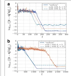
Note that both errors are calculated from the network (global) perspective and as depicted, they are not known locally at the nodes, since only R(k)(t) is local at each node, whereas Q(t) is distributed row-wise across the nodes (Qk(t)). From now on, we simplify the notation by dropping the index t inQ(t) andR(k)(t). The simu-lation results for a geometric topology with an average node degree d¯ = 8.533 are depicted in Fig. 1. Since both errors behave almost identically (compare Fig. 1a, b) and since each node k can compute a local factor-ization errorAk−QkR(k)2/Ak2from its local data, we conjecture that such local error evaluation can be used also as a local stopping criterion in practice. Note that this fact was used in [26] for estimating a network size.
Note that the error at the beginning stage in Fig. 1 is caused by the disagreement and not converged norms and inner products across the nodes, i.e., the values of
˜
U(t),Q˜(t),P˜(1)(t), andP˜(2)(t). We also observe that the error floor4 is highly influenced by the network topol-ogy, weights of matrixW, and condition number of input matrixA. We investigate these properties in Section 5.3.
5.2 Initial data distribution
If n > N, some nodes store more than one row of A. Thus, before doing distributed summation (broadcasting to neighbors), every node has to locally sum the values of its local rows.
Fig. 1Example of orthogonality (a) and factorization error (b) for each node k for a geometric topology withd=8.533.N=30,k=1, 2,. . ., 30
rows are stored in the node with the highest degree, the rest in the remaining 29 nodes.
We observe that not only the initial distribution of the data influences the convergence behavior but also the topology of the underlying network. In the case of a reg-ular topology (Fig. 2a), the influence of the distribution is small and relatively weak in terms of convergence time but stronger in terms of the final accuracy achieved. We rec-ognize that the difference between the nodes comes only from the variance of the values in input matrixA. On the other hand, in case of a highly irregular geometric topol-ogy (see Fig. 2b), where the node with most neighbors stores most of the data, the algorithm converges much faster than in the case when most of the data are stored in a node with only few neighbors.
We further observe that in the “uniform” case, the algorithm behaves slightly differently for different distri-butions of the rows (although still having ten rows in each node). In Fig. 3, we show results for six different placements of the data across the nodes for three dif-ferent topologies, where we depict the mean value and the corresponding confidence intervals of the simulated orthogonality error. As we can observe, in case of the fully connected topology, the data distribution is of no impor-tance, since all the nodes exchange data in every step with all other nodes. In case of the geometric topology,
Fig. 2Convergence for networks with different topology and initial data distribution: either all nodes store the same amount of data (“uniform”) or most of the data is stored in one node (with minimum or maximum degree) (a- Regular topology withd=5;b- Geometric topology withd=5). In case of the regular topology (a), the nodesi,j
are picked randomly
however, the convergence of the algorithm is influenced by the distribution of data, even if every node contains the same number of rows (ten rows in each node). This can be recognized by bigger confidence intervals of the orthog-onality error. Nevertheless, the speed of convergence for all cases is bigger than the case when most data is stored in the “sparsest” node (cf. Fig. 2b). In case of the regu-lar topology, the difference is small only due to numerical accuracy of the mixing parameters.
Fig. 3“Uniform” distribution for different topologies. (Boldface lineis the mean value across six different uniform data distributions.Shaded
5.3 Numerical sensitivity
As mentioned in Section 3.1, the classical Gram-Schmidt orthogonalization possesses some undesirable numerical properties [1, 23]. In comparison to centralized algo-rithms, numerical stability of DS-CGS is furthermore influenced by the precision of the mixing weight matrix
W, the network topology, and properties of input matrixA, i.e., its condition number (see Fig. 5 ahead) and the distribution of the numbers in the rows of the matrix (see Figs. 2 and 3). In this section, we provide simulation results showing these dependencies.
5.3.1 Weights
As mentioned in Section 2, matrixWcan be selected in many ways. Mainly, the selection of the weights influences the speed of convergence. Unlike previous simulations, where we used the metropolis weights (see Eq. (2)), here we selected constant weights for matrixW[20], i.e.,
[W]ij= ⎧ ⎪ ⎨ ⎪ ⎩ c
N if(i,j)∈E, 1−Ncdi ifi=j, 0 otherwise,
(8)
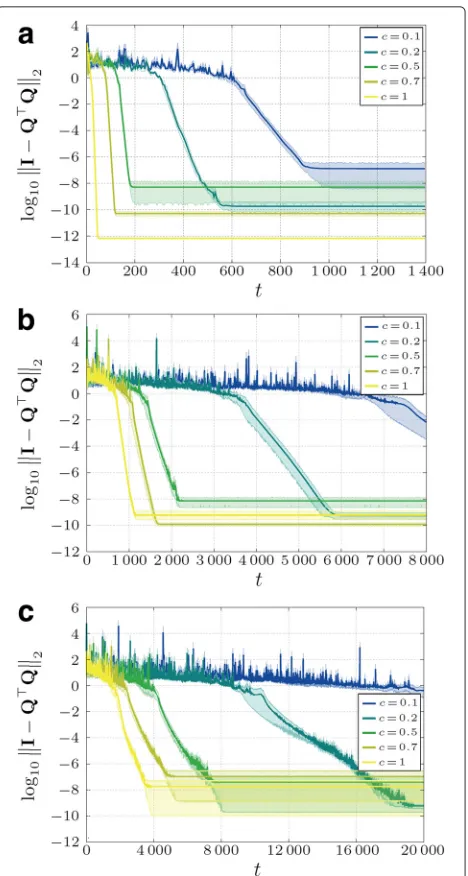
wherec∈ (0, 1]. Such weights, in general, lead to slower convergence. However, we can also see in Fig. 4 that the weights influence not only the speed of convergence but also the numerical accuracy of the algorithm (different error floors).
5.3.2 Condition numbers
It is well known that the classical Gram-Schmidt orthog-onalization is numerically unstable [23]. In cases when input matrix A is ill-conditioned (high condition num-ber) or rank-deficient (matrix contains linear dependent columns), the computed vectorsQcan be far from orthog-onal even when computed with high precision.
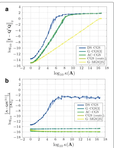
In this section, we study the influence of the con-dition number of input matrix A on the accuracy of the orthogonality. The condition number is defined with respect to inversion as the ratio of the largest and small-est singular value. In comparison to classical (centralized) Gram-Schmidt orthogonalization, we observe (Fig. 5a) that the DS-CGS algorithm behaves similarly, although it reaches neither the accuracy of AC-CGS nor of the cen-tralized algorithm (even in the fully connected network). We observe in all of the simulations that the orthogonality error in the first phase can reach very high values (due to divisions by numbers close to zero), which may influence the numerical accuracy in the final phase.
We further observe that the algorithm requires matrixA
to be very well-conditioned even for the fully connected network. Unlike other methods, the factorization error in case of DS-CGS has the same characteristics as the orthogonality error and is also influenced by the condition number of the input matrix, see Fig. 5b. Although, as we
Fig. 4Influence of different constant weightsc(Eq. (8)) on the algorithm’s accuracy and convergence speed for three different topologies (a- Fully connected topology;b- Regular topology;
c- Geometric topology) averaged over ten different input matrices (a–c). (Shaded areasare 95 % confidence intervals)
noted in Section 5.1, orthogonality and factorization error of DS-CGS behave almost identically, the dependence of condition numberκ(A)on the factorization error would need a further investigation.
Figure 5 also shows that G-MGS is the most robust method in comparison to the others. This is caused by the usage of the modified Gram-Schmidt orthogonalization instead of the classical one.
5.3.3 Mixing precision
Fig. 5Impact of the condition numberκ(A)of matrixAon the orthogonality (a) and factorization error (b). Averaged over ten matrices for each condition number. Fully connected network. (Both axesare in logarithmic scale.Shaded areasare 95 % confidence intervals)
we simulate the case of a geometric topology with the Metropolis weights model, where the weights are of given precision—characterized by the number of variable deci-mal digits (4, 8, 16, 32, “Infinite”).5
If we compare Fig. 6 with Fig. 7, we find that the numer-ical precision of the mixing weights have bigger influence in cases when the input matrix is worse conditioned. In Figs. 8 and 9, we can see the difference between
Fig. 6Influence of the numerical precision of the mixing weights on the orthogonality error of DS-CGS. Geometric topology, matrixAwith low condition number (κ(A)=1.04)
Fig. 7Influence of the numerical precision of the mixing weights on the orthogonality error of DS-CGS. Geometric topology, matrixAwith higher condition number (κ(A)=76.33)
orthogonality errors for various precisions. We observe that for the matrixAwith higher condition number, the higher mixing precision has bigger impact on the result.
As we find in Fig. 6, the error floor moves with the mix-ing precision. However, we must note that even for the “infinite” mixing precision the orthogonality error stalls at an accuracy (∼10−12) lower than the used machine precision—taking into account also the conversion to dou-ble precision. From the simulations, we conclude that this is caused by high numerical dynamic range in the first phases of the algorithm as well as by the errors created by the misagreement among the nodes during the transient phase of the algorithm.
5.4 Robustness to link failures
In case of distributed algorithms, it is of big importance that the algorithm is robust against network failures. Typ-ical failures in WSN are message losses or link failures, which occur due to many reasons, e.g., channel fad-ing, congestions, message collisions, moving nodes, or dynamic topology.
We model link failures as a temporary drop-out of a bidirectional connection between two nodes, meaning
Fig. 8Difference in the orthogonality errorlog10I−QQ(2vpa−i)
Fig. 9Difference in the orthogonality errorlog10I−QQ(2vpa−16)
− I−QQ(2Inf)for the case of 16 decimal digits versus “infinite” precision (converted to double). Note that in comparison to Fig. 8, the difference between “infinite” and more than 16 digits is below the machine precision (exact same results)
that no message can be transmitted between the nodes. In every time step, we randomly remove some per-centage of links in the network. As a weight model, we picked the constant weights model, Eq. (8), due to its property that every node can compute at each time step the weights locally based only on the num-ber of received messages (di). Thus, no global knowl-edge is required. However, the nodes must still work synchronously.6
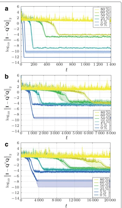
From Fig. 10, we conclude that the algorithm is very robust and even if we drop in every time step, a big percentage (up to 60 %) of the links, the algorithm still achieves some accuracy (at least 10−2; Fig. 10c).
It is worth noting that moving nodes and dynamic net-work topology can be modeled in the same way. We therefore argue that the algorithm is robust also to such scenarios (assuming that synchronicity is guaranteed).
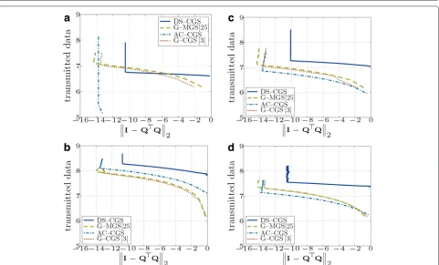
5.5 Performance comparison with existing algorithms We compare our new DS-CGS algorithm with AC-CGS, G-AC-CGS, and G-MGS introduced in Section 3.2. Although all approaches have iterative aspects, the cost per iteration strongly differs for each algorithm. Thus, instead of providing a comparison in terms of number of iterations to converge, we compare the communi-cation cost needed for achieving a certain accuracy of the result. We investigate the total number of messages sent as well as the total amount of data (real numbers) exchanged.
Simulation results for various topologies are shown in Figs. 11 and 12. The gossip-based approaches exchange, in general, less data (Fig. 12), but since their message size is much smaller than in DS-CGS, the total number of messages sent is higher (Fig. 11).
Because the message size of AC-CGS is even smaller than in the gossip-based approaches, it sends the high-est number of messages. Since the energy consumption in
Fig. 10Robustness to link failures for different percentages of failed links at every time step (a- Fully connected;b- Regular topology;c -Geometric topology). Constant weight model withc=1, i.e., the fastest option (see Fig. 4). (Shaded areasare 95 % confidence intervals)
a WSN is mostly influenced by the number of transmis-sions [36, 37], it is better to transmit as few messages as possible (with any payload size); therefore, DS-CGS is the most suitable method for a WSN scenario. However, we notice that in many cases, DS-CGS does not achieve the same final accuracy of the result as the other methods.
Note that in fully connected networks, AC-CGS deliv-ers a highly accurate result from the beginning, because within the first iterations, all nodes exchange the required information with all other nodes.
Fig. 11Total number of transmitted messages in the network vs. orthogonality error (both axesare inlogarithmicscale log10) (a- Fully connected topology;b- Geometric topology withd=8.53;c- Geometric topology withd=24.46;d- Regular topology withd=5)
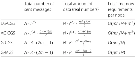
Table 1Comparison of various distributed QR factorization algorithms
Total number of Total amount of Local memory sent messages data (real numbers) requirements
per node
I(d)denotes the number of iterations of “dynamic” consensus,I(s)the number of
iterations of “static” consensus,Rthe number of rounds per push-sum,Nthe number of nodes,mthe number of columns of the input matrix
number of iterationsI(s)andI(d)required for convergence in “static” and “dynamic” consensus-based algorithms or the number of roundsRneeded for convergence of push-sum in the gossip-based approaches. For example, in a fully connected network R = O(logN) [24], I(s) =
1. Thus, AC-CGS requires O(m2N) messages sent as well as data exchanged, whereas gossip-based approaches need O(mNlogN) messages and O(m2NlogN) data. Note that G-CGS and G-MGS have theoretically iden-tical communication cost; however, G-MGS is numer-ically more stable (see Fig. 5) and achieves a higher final accuracy (see Figs. 11 and 12). In case of DS-CGS and a fully connected network, we can interpret DS-CGS in the worst case as m consequent static con-sensus algorithms (one for each column); thus, I(d) = O(m), and the number of transmitted messages isO(mN)
and dataO(m3N). Nevertheless, theoretical convergence bounds of DS-CGS (on I(d)) remain an open research question.
6 Conclusions
We presented a novel distributed algorithm for comput-ing QR decomposition and provided an analysis of its properties. In contrast to existing methods, which com-pute the columns of the resulting matrixQconsecutively, our method iteratively refines all elements at once. Thus, in any moment, the algorithm can deliver an estimate of both matrices Q and R. The algorithm dramatically outperforms known distributed orthogonalization algo-rithms in terms of transmitted messages, which makes it suitable for energy-constrained WSNs. Based on our empirical observation, we argue that the evaluation of the local factorization error at each node might lead to a suitable stopping criterion for the algorithm. We also provided a thorough study of its numerical properties, analyzing the influence of the precision of the mixing weights and condition numbers of the input matrix. We furthermore analyzed the robustness of the algorithm to link failures and showed that the algorithm is capable to
reach a certain accuracy even for a high percentage of link failures.
The biggest drawback of the algorithm is the neces-sity to have synchronously working nodes. This leads to poor robustness when the messages are sent (or lost) asyn-chronously. As we showed, since the algorithm originates from the classical Gram-Schmidt orthogonalization, also the numerical sensitivity of the algorithm is a big issue and needs to be addressed in the future. The optimization of the weights and design of algorithm in such way that it avoids a big dynamic numerical range, especially in the first phases, is also of interest.
An alternative approach, not considered here, which could be worth of future research, would be to find a distributed algorithm as an optimization problem, e.g., mins.t.QQ=IA− QR. In literature, there exist many
distributed optimization methods, e.g., [38, 39], which could lead to even superior algorithms, with even faster convergence and smaller error floors.
Last but not least, theoretical bounds of DS-CGS for the convergence time and rate remain an open issue. A first application of the algorithm has already been proposed in [26]. Also, since the proposed algorithm is not restricted to the usage in wireless sensor networks only, a transfer of the proposed algorithm onto so-called network-on-chip platforms [40] could possibly lead to further new interesting and practical applications as well.
Endnotes
3Not considering numerical properties.
4Error level at which the algorithm stalls at given computational precision.
5The simulations were performed in Matlab R2011b 64-bit using the Symbolic Math Toolbox with variable precision arithmetic. “Infinite” precision denotes weights represented as an exact ratio of two numbers. The depicted result after “infinite” precision multiplication was converted to double precision.
6If there is a link, nodes see each other and
immediately exchange messages. From a mathematical point of view, this implies that weight matrixWwill be doubly stochastic [1] in every time step.
Appendix: local algorithm
1. Initialization (t=0). Nodei stores the following
(b) Store the local part of the resulting matrixQ and the whole matrixR, i.e.,
(c) Aggregate the following data into one message:
ψ(1)
(d) Broadcast the message containing the vectors neighbors and update the own local data
The authors declare that they have no competing interests.
Acknowledgements
This work was supported by the Austrian Science Fund (FWF) under project grants S10608-N13 and S10611-N13 within the National Research Network SISE. Preliminary parts of this work were previously published at the 46th Asilomar Conf. Sig., Syst., Comp., Pacific Grove, CA, USA, Nov. 2012 [32].
Author details
1TU Wien, Institute of Telecommunications, Gusshausstrasse 25/E389, 1040 Vienna, Austria.2University of Vienna, Faculty of Computer Science, Theory and Applications of Algorithms, Währingerstrasse 29, 1090 Vienna, Austria.
Received: 28 May 2015 Accepted: 10 February 2016
References
1. GH Golub, CF Van Loan,Matrix Computations, 3rd Ed. (Johns Hopkins Univ. Press, Baltimore, USA, 1996)
2. JM Lees, RS Crosson, inSpatial Statistics and Imaging, ed. by A Possolo. Bayesian ART versus conjugate gradient methods in tomographic seismic imaging: an application at Mount St. Helens, Washington, vol. 20 (IMS Lecture Noted-Monograph Series, Hayward, CA, 1991), pp. 186–208 3. C Dumard, E Riegler, inInt. Conf. on Telecom. ICT ’09. Distributed sphere
decoding (IEEE, Marrakech, 2009), pp. 172–177
4. G Tauböck, M Hampejs, P Svac, G Matz, F Hlawatsch, K Gröchenig, Low-complexity ICI/ISI equalization in doubly dispersive multicarrier systems using a decision-feedback LSQR algorithm. IEEE Trans. Signal Process.59(5), 2432–2436 (2011)
5. E Hänsler, G Schmidt,Acoustic Echo and Noise Control. (Wiley, Chichester, New York, Brisabne, Toronto, Singapore, 2004)
6. PSR Diniz,Adaptive Filtering—Algorithms and Practical Implementation. (Springer, US, 2008)
7. AH Sayed,Adaptation, Learning, and Optimization over Networks, vol. 7. (Foundations and Trends in Machine Learning, Boston-Delft, 2014) 8. K-J Cho, Y-N Xu, J-G Chung, inIEEE Workshop on Signal Processing Systems.
Hardware efficient QR decomposition for GDFE (IEEE, Shanghai, China, 2007), pp. 412–417
9. X Wang, M Leeser, A truly two-dimensional systolic array FPGA implementation of QR decomposition. ACM Trans. Embed. Comput. Syst. 9(1), 3–1317 (2009)
10. A Buttari, J Langou, J Kurzak, J Dongarra, inProc. of the 7th International Conference on Parallel Processing and Applied Mathematics. Parallel tiled QR factorization for multicore architectures (Springer, Berlin, Heidelberg, 2008), pp. 639–648
11. J Demmel, L Grigori, MF Hoemmen, J Langou, Communication-optimal parallel and sequential QR and LU factorizations (2008). Technical report, no. UCB/EECS-2008-89, EECS Department, University of California, Berkeley 12. F Song, H Ltaief, B Hadri, J Dongarra, inInternational Conference for High
Performance Computing, Networking, Storage and Analysis. Scalable tile communication-avoiding QR factorization on multicore cluster systems (IEEE Computer Society, Washington, DC, USA, 2010), pp. 1–11 13. M Shabany, D Patel, PG Gulak, A low-latency low-power
QR-decomposition ASIC implementation in 0.13μm CMOS. IEEE Trans. Circ. Syst. I.60(2), 327–340 (2013)
14. A Nayak, I Stojmenovi´c,Wireless Sensor and Actuator Networks: Algorithms and Protocols for Scalable Coordination and Data Communication. (Wiley, Hoboken, NJ, 2010)
15. H Straková, WN Gansterer, T Zemen, inProc. of the 9th International Conference on Parallel Processing and Applied Mathematics, Part I. Lecture Notes in Computer Science. Distributed QR factorization based on randomized algorithms, vol. 7203 (Springer Berlin Heidelberg, Berlin, Heidelberg, 2012), pp. 235–244
17. O Sluˇciak, M Rupp, inProc. of the 36th IEEE International Conference on Acoustics, Speech and Signal Processing (ICASSP). Reaching consensus in asynchronous WSNs: algebraic approach, (Prague, 2011), pp. 3300–3303. Chap. Acoustics, Speech and Signal Processing (ICASSP), 2011 18. O Sluˇciak, M Rupp, inProc. of Statistical Sig. Proc. Workshop (SSP). Almost
sure convergence of consensus algorithms by relaxed projection mappings (IEEE, Ann Arbor, MI, USA, 2012), pp. 632–635
19. F Sivrikaya, B Yener, Time synchronization in sensor networks: a survey. IEEE Netw. Mag. Special Issues Ad Hoc Netw. Data Commun. Topol. Control.18(4), 45–50 (2004)
20. R Olfati-Saber, JA Fax, RM Murray, Consensus and cooperation in networked multi-agent systems. Proc. IEEE.95(1), 215–233 (2007) 21. L Xiao, S Boyd, Fast linear iterations for distributed averaging. Syst. Control
Lett.53, 65–78 (2004)
22. L Xiao, S Boyd, S Lall, inProc. ACM/IEEE IPSN–05. A scheme for robust distributed sensor fusion based on average consensus (IEEE, Los Angeles, USA, 2005), pp. 63–70
23. LN Trefethen, D Bau III,Numerical Linear Algebra. (SIAM: Society for Industrial and Applied Mathematics, Philadelphia, 1997), p. 373 24. D Kempe, A Dobra, J Gehrke, inFoundations of Computer Science, 2003.
Proceedings. 44th Annual IEEE Symposium on. Gossip-based computation of aggregate information, (2003), pp. 482–491. ISSN:0272-5428, doi:10.1109/SFCS.2003.1238221
25. H Straková, WN Gansterer, in21st Euromicro Int. Conf. on Parallel, Distributed, and Network-Based Processing (PDP). A distributed eigensolver for loosely coupled networks (IEEE, Belfast, UK, 2013), pp. 51–57 26. O Sluˇciak, M Rupp, Network size estimation using distributed
orthogonalization. IEEE Sig. Proc. Lett.20(4), 347–350 (2013) 27. P Braca, S Marano, V Matta, inProc. Int. Conf. Inf. Fusion (FUSION 2008).
Running consensus in wireless sensor networks (IEEE, Cologne, Germany, 2008), pp. 152–157
28. W Ren, inProc. of the 2007 American Control Conference. Consensus seeking in multi-vehicle systems with a time-varying reference state (IEEE, New York, NY, 2007), pp. 717–722
29. V Schwarz, C Novak, G Matz, inProc. 43rd Asilomar Conf. on Sig., Syst., Comp. Broadcast-based dynamic consensus propagation in wireless sensor networks (IEEE, Pacific Grove, CA, 2009), pp. 255–259 30. M Zhu, S Martínez, Discrete-time dynamic average consensus.
Automatica.46(2), 322–329 (2010)
31. O Sluˇciak, O Hlinka, M Rupp, F Hlawatsch, PM Djuri´c, inRec. of the 45th Asilomar Conf. on Signals, Systems, and Computers. Sequential likelihood consensus and its application to distributed particle filtering with reduced communications and latency (IEEE, Pacific Grove, CA, 2011), pp. 1766–1770
32. O Sluˇciak, H Straková, M Rupp, WN Gansterer, inRec. of the 46th Asilomar Conf. on Signals, Systems, and Computers. Distributed Gram-Schmidt orthogonalization based on dynamic consensus (IEEE, Pacific Grove, CA, 2012), pp. 1207–1211
33. P Braca, S Marano, V Matta, AH Sayed, inProc. of the 39th IEEE International Conference on Acoustics, Speech and Signal Processing (ICASSP). Large deviations analysis of adaptive distributed detection (IEEE, Florence, Italy, 2014), pp. 6153–6157
34. O Sluˇciak, Convergence analysis of distributed consensus algorithms (2013). PhD thesis, TU Vienna
35. B Efron, RJ Tibshirani,An Introduction to the Bootstrap. (Chapman & Hall/CRC Monographs on Statistics & Applied Probability 57, London, UK, 1994)
36. P Rost, G Fettweis, inGLOBECOM Workshops, 2010 IEEE. On the
transmission-computation-energy tradeoff in wireless and fixed networks (IEEE, Miami, FL, 2010), pp. 1394–1399
37. R Shorey, A Ananda, MC Chan, WT Ooi,Mobile, Wireless, and Sensor Networks: Technology, Applications, and Future Directions. (Wiley, Hoboken, NJ, 2006)
38. B Johansson, On distributed optimization in networked systems (2008). PhD thesis, KTH, Stockholm
39. I Matei, JS Baras, Performance evaluation of the consensus-based distributed subgradient method under random communication topologies. IEEE J. Sel. Top. Signal Process.5(4), 754–771 (2011) 40. L Benini, GD Micheli, Networks on chips: a new SoC paradigm. IEEE
Comput.35(1), 70–78 (2002)
Submit your manuscript to a
journal and benefi t from:
7Convenient online submission
7Rigorous peer review
7Immediate publication on acceptance
7Open access: articles freely available online
7High visibility within the fi eld
7Retaining the copyright to your article