R E S E A R C H
Open Access
Robust and adaptive diffusion-based
classification in distributed networks
Patricia Binder
*, Michael Muma and Abdelhak M. Zoubir
Abstract
Distributed adaptive signal processing and communication networking are rapidly advancing research areas which enable new and powerful signal processing tasks, e.g., distributed speech enhancement in adverse environments. An emerging new paradigm is that of multiple devices cooperating in multiple tasks (MDMT). This is different from the classical wireless sensor network (WSN) setup, in which multiple devices perform one single joint task. A crucial first step in order to achieve a benefit, e.g., a better node-specific audio signal enhancement, is the common unique labeling of all relevant sources that are observed by the network. This challenging research question can be addressed by designing adaptive data clustering and classification rules based on a set of noisy unlabeled sensor observations. In this paper, two robust and adaptive distributed hybrid classification algorithms are introduced. They consist of a local clustering phase that uses a small part of the data with a subsequent, fully distributed on-line classification phase. The classification is performed by means of distance-based similarity measures. In order to deal with the presence of outliers, the distances are estimated robustly. An extensive simulation-based performance analysis is provided for the proposed algorithms. The distributed hybrid classification approaches are compared to a benchmark algorithm where the error rates are evaluated in dependence of different WSN parameters. Communication cost and computation time are compared for all algorithms under test. Since both proposed approaches use robust estimators, they are, to a certain degree, insensitive to outliers. Furthermore, they are designed in a way that they are applicable to on-line classification problems.
Keywords: Adaptive distributed classification, Clustering, Labeling, Robust, Outlier, Multi device multi task (MDMT)
1 Introduction
Recent advances in distributed adaptive signal process-ing and communication networkprocess-ing are currently enablprocess-ing novel paradigms for signal and parameter estimation. Based on the principles of adaptive filtering theory [1], a network of devices with node-specific interests adaptively optimizes its behavior, e.g., to jointly solve a decentral-ized least mean squares problem [2–6]. Under this new paradigm, multiple devices cooperate in multiple tasks (MDMT). This is different from the classical wireless sen-sor network setup, in which multiple devices perform one single joint task [2].
The MDMT paradigm can be beneficial, e.g., for speech enhancement in adverse environments [7]. Consider, for example, distributed audio signal enhancement in a public
*Correspondence: [email protected]
Signal Processing Group, Technische Universität Darmstadt, 64283 Darmstadt, Germany
area, such as an airport, a train-station, etc. By cooperat-ing with each other, various devices (e.g., smart-phones, hearing aids, tablets) benefit in enhancing their node-specific audio source of interest, given a received mixture of interfering sound sources [2, 8], e.g., by suppressing noise and interfering sound sources that are not of interest to the user.
Note that in such scenarios, the devices must operate under stringent power and communication constraints and the transmission of observations to a fusion cen-ter (FC) is, in many cases, infeasible or undesired. A crucial first step in order to achieve a benefit, e.g., a bet-ter node-specific audio signal enhancement, is the com-mon unique labeling of all relevant speech sources that are observed by the network [8]. Also in other MDMT signal-enhancement tasks, such as image enhancement, it is of practical importance to answer the question: who observes what? [9].
This challenging research question can be tackled by designing adaptive data clustering and classification rules where each sensor collects a set of unlabeled observa-tions that are drawn from a known number of classes. In particular, object or speaker labeling can be solved by in-network adaptive classification algorithms where a minimum amount of information is exchanged among single-hop neighbors. Various methods have been pro-posed that deal with distributed data clustering and classification, e.g., [8–24]. In the last few years, sev-eral distributed adaptive strategies, such as incremental, consensus, and diffusion least mean squares algorithms have been developed [25]. In [17], a distributed K-Means (DKM) algorithm that uses the consensus strategy was proposed.
In this paper, we provide an adaptive and robust hybrid diffusion-based approach which extends our previously published algorithm [21] by a robust distance measure that improves the classification/labeling per-formance, especially if the covariances of the clusters differ significantly. Robust methods become necessary whenever the distribution of the extracted features is heavy tailed or contains outliers [26, 27] due to errors in the feature estimation step. A scenario contain-ing a high amount of outliers, as depicted in Fig. 1, complicates the classification considerably. In such a scenario, we propose to base the classification/labeling on robust adaptive centroid estimation and data clustering.
Contributions: Two robust in-network distributed classification algorithms, i.e., the RDiff K-Med and the CE RDiff K-Med, are proposed. It is shown that the perfor-mance of the first algorithm can be approached by the sec-ond algorithm with a considerably lower between-sensor communication cost. Unlike the DKM, which serves as a benchmark, the proposed algorithms are adaptive, instead
−4 −2
0 2
4 6
−5 0 5 10 −4 −2 0 2 4 6 8 10
x y
z
Fig. 1Three data clusters containing outlying feature vectors
of working with a batch of data. They are thus applica-ble to real-time classification proapplica-blems. Furthermore, they are robust against outliers in the feature vectors and can handle non-stationary features. An extensive simulation-based performance analysis is provided that investigates the error rates in dependence of different WSN parame-ters, and also considers communication cost and compu-tation time.
Organization:Section 2 provides the problem formula-tion, Section 3 provides a brief introduction to the topic of robust estimation of class centroid and covariance. Section 4 is dedicated to the proposal and description of two robust diffusion-based classification algorithms, while Section 5 provides an extensive Monte-Carlo simu-lation study. Section 6 concludes the paper and provides future research directions.
2 Problem formulation and data model
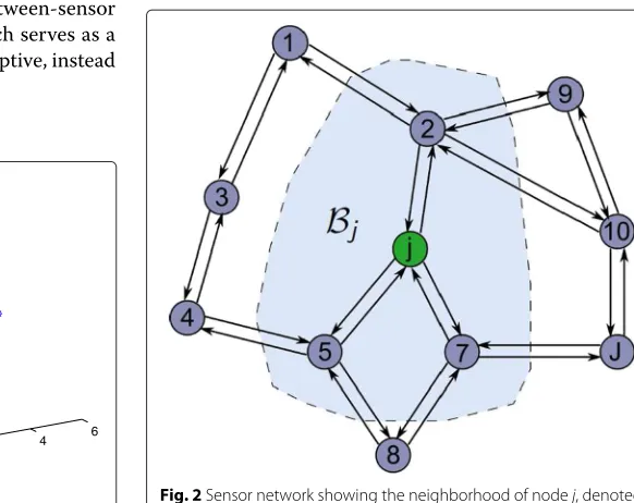
Consider a network with J nodes distributed over some geographic region (see Fig. 2). Two nodes are con-nected if they are able to communicate directly with each other. The set of nodes connected to node j ∈ 1,. . .,J =: J is called the neighborhood of node j and is denoted by Bj ⊆ J. The communication links
between the nodes are symmetric and a node is always connected to itself. The number of nodes connected to node j is called the degree of node j and is denoted by|Bj|.
This paper is concerned with adaptive data cluster-ing and classification/labelcluster-ing when each sensor collects
a set of unlabeled observations that are drawn from a known number of classes. This task should be accom-plished in a decentralized manner by communicating only within directly connected neighborhoodsBj, instead
of transmitting all observations to a master node or FC. Each observation is assumed to belong to a cer-tain class Ck with k ∈ 1,. . .,K with k denoting the
label of the given class. The total number of classes K is assumed to be known, or estimated a priori. Each class is described by a number of application depen-dent descriptive statistics (features). The feature estima-tion process is an applicaestima-tion-specific research area of its own (see, e.g., [8, 9]) and is not considered in this article, where we seek for generic adaptive robust clus-tering and classification methods. In the following, it is assumed that the feature extraction has already been performed, so that the uncertainty of the feature estima-tion within each class can be modeled by a probability distribution, e.g., the Gaussian. Further, we account for estimation errors in the feature extraction process that we consider as outliers, thus arriving at the following observation model for feature vectors at time instant n,n=1,. . .,N:
djkn=wk+ejkn+ojn. (1)
Here,wkdenotes the class centroid,ejknrepresents the
class-specific uncertainty term with covariance matrix jk, ojn denotes the outlier term which models
distur-bances of an unspecified density and djkn,wk,ejkn ∈
Rq. e
jkn is assumed to be temporally and spatially
independent, i.e.,
E{e∗jnelm} =σe2,j·δjl·δnm (2)
with j,l = 1,. . .,J, n,m = 1,. . .,N and δ denot-ing the Kronecker delta function. ejkn is assumed to
be zero mean. For reasons of clarity, we drop the index k in the observation vectors and refer to them asdjn.
The aim of this paper is thus to enable every node j to assign each observation to a cluster k based on an estimated feature djn. The classification/labeling should
be real-time capable so that a new observation can be assigned on-line without the necessity of all recorded observations being available. Furthermore, outliers in Eq. (1) should not have a huge effect on the labeling performance. This will be achieved by using robust tech-niques to estimate the class centroids and covariances, as well as robust distance measures, as described in the next section.
3 Robust estimation of class centroid and
covariance
The presence of even a small amount of outliers in a data set can have a high impact on classical estimators like the sample mean vector and sample covariance matrix. Though these estimators are optimal under the Gaus-sian noise assumption, they are extremely sensitive to uncharacteristic observations in the data [26]. For this purpose, robust estimators have been developed which are, to a certain degree, resistant towards outliers in the data.
In the following, a short overview of the con-cept of M-estimation for the multivariate case is pre-sented, as required by our methods. For a more detailed treatment of the fundamental concepts, see, e.g., [26, 28].
The hybrid classification approach developed in this paper involves estimating the mean and covariance for vector-valued data djn = (d1jn,d2jn,. . .,dqjn)T with
djn ∈ Rq, where q is the dimension of the feature
space.
In the univariate case, it is possible to define the robust estimates of location and dispersion separately. In the multivariate case, In order to obtain equivariant estimates, it is of advantage to estimate location and dispersion simultaneously [28].
The multivariate Gaussian density is
fD(d;w,)=
the form (3). M-estimates of the cluster centroids and covariance matrices are defined as solutions of the general system equations
where the functions φ1 and φ2 may be chosen
differ-ently. Uniqueness of solutions of (4) and (5) requires that gDφ2(gD)is a nondecreasing function ofgD[28].
A common choice areHuber’s functions[29] with
ρ(d)=
d2jn , if |djn|≤chub
2chub|djn| −chub2 , if |djn|>chub
and
φ1,2(d)= ∂ρ( d)
∂d (7)
withchubdenoting the Huber’s tuning constant. The
func-tion ρ(d) from Eq. (6) shows quadratic behavior in the central region while increasing linearly to infinity. Outliers are therefore assigned less weight than data close to the model. Note that all maximum likelihood estimators are also M-estimators.
4 Proposed methods
In this section, two new robust in-network distributed classification algorithms are presented that extend our previously published algorithm [21] by a robust distance measure that improves the classification/labeling perfor-mance, especially if the covariances of the clusters differ significantly.
Since we have no training data available for the classifi-cation process, the general idea of the methods is to split the classification/labeling procedure into two main steps: in alocal clustering phaseeach node calculates a prelimi-nary estimate of the cluster characteristics (i.e., centroids and covariances) of each cluster using a small number of feature vectors. These preliminary estimates serve as an initialization for the subsequent global classification phase. Here, based on these estimates, a new feature is classified using a robust distance measure. The aim is to improve the local classification result by a combina-tion of local processing and communicacombina-tion between the agents.
An advantage of this procedure is that this hybrid approach turns into a mere classification algorithm when the cluster characteristics are known before-hand. In this case, the local clustering phase is not needed.
The methods are based on the diffusion LMS strategy that was introduced in [30]. In this way, the classifica-tion is adaptive and can handle streaming data coming from a distributed sensor network. Since the communi-cation cost between the nodes should be kept as low as possible, the second approach is designed with reduced in-network communication. A robust design makes sure that the proposed algorithms are, to a certain degree, resistant towards outliers in the feature vectors. In the following, the two proposed approaches are described in detail.
4.1 Robust distance-based K-medians
clustering/classification over adaptive diffusion networks (RDiff K-Med)
The first proposed hybrid classification methodology is the “Robust Distance-Based Clustering/Classification
Algorithm over Adaptive Diffusion Networks” (RDiff K-Med). It begins with a local initialization phase where each nodejcollects a number ofNtobservations and performs
K-medians clustering on these observations. In this way, each node locally partitions its firstNtobservationsDjn=
{djn,n = 1,. . .,Nt}intoksetsCk so that the1-distance
within each cluster is minimized:
arg min
Each center is the component-wise median of the points of each cluster. The features assigned to each classCkare
stored in an initial feature matrix S0jk. Based on all ele-ments in S0jk, local intermediate estimates of the cluster centroidψ0jkand covariance matrix0jkare determined. In the following, the calculation steps are presented in detail. First, as robust local initial estimate of the cluster center, compute the column-wise median ofS0jk
ˆ
ψ0jkis thus obtained by computing the median separately
for each spatial direction of all elements inS0jk.
Next, proceed by computing a robust local initial esti-mate of the cluster covariances. In this paper, we compare three estimators, i.e. the sample covariance, Huber’s M-estimator and a computationally simple robust covariance estimator based on the median absolute deviation (MAD).
The sample covariance matrix estimate is given by
ˆ
Huber’s M-estimator, as defined in Eq. (6), is computed via an iteratively reweighted least-squares algorithm, as detailed in [28] with the previously computed ψˆ0jk as location estimate.
In case of the MAD based covariance estimate, for each featuredjninS0jkthe difference vector
ddiff,jk= |djn−median
S0jk
| (11)
and the corresponding covariance matrix is
ˆ
0jk(r,s)= σˆ
0
jks 2
, ∀r=s=1,. . .,q
0, ∀r =s (13)
with σˆ0jks denoting the standard deviation estimate in each spatial direction of the feature space. Note that the covariance matrix calculated in Eq. (13) is a diagonal matrix. This computationally simple robust estimator is only applicable when the entries of the feature vectors are assumed to be independent of each other. The estimates of the sample covariance matrix and the M-estimator do not require this assumption and are, in general, not diagonal matrices.
Since the order in which the cluster centroids are stored by K-Medians is random, it may differ between two nodes. Thus, it has to be assured that the data which is exchanged by the nodes refers to the same classes. This is achieved by a unique initial ordering of the class centroids and covari-ance matrices among all nodes in the network: starting with the class centroids and covariance matrices stored for the first class of a preset reference node, all other nodes calculate the Euclidean distance of the respective entries corresponding to all stored classes and those of the first class of the reference node. The data with the smallest Euclidean distance to the reference entries are re-stored at the position corresponding to the first class. This proce-dure is repeated for all classes stored by the nodes in the network.
Having obtained a consistent data structure, each node jexchanges its own feature vectorsS0jk for each classCk
with its neighborsi ∈ Bj. All nodes store their own as
well as the features received from their neighbors in an initial matrixV0jk. In the following clustering/classification
procedure,S0jk andV0jk are extended to Sjkn andVjkn in
every time stepnby adding columns containing the new feature vectors received at time stepn.
This completes the initialization phase, which is fol-lowed by the exchange phase, where each new observation djn, n = Nt + 1,. . .,N, is classified according to the
following diffusion-procedure:
1. Exchange Step:If there are new, unshared feature vec-tors, each nodejadds them toVjknand broadcasts them
to its neighborsi∈Bj.
2. Adaptation Step:Each nodejdetermines preliminary local estimatesψˆjkn andˆ∗jkn at timenbased on the fea-ture vectors stored inVjknanalogously to –(13) withVjkn
replacingSjkn. In order to be capable of dealing with
non-stationary time-varying signals, a window length lw is
introduced which limits the size ofVjknby only retaining
the latestlwelements which were added toVjkn.
3. Exchange Step:Each node exchanges its intermediate estimatesψˆjknandˆ∗jknwith its neighbors.
4. Combination Step: Each node jadapts its estimates according to
ˆ
wjkn=α· ˆψjkn+(1−α)·
b∈Bj/{j}
abkn· ˆψbkn (14)
and
ˆ
jkn=α· ˆ
∗
jkn+(1−α)·
b∈Bj/{j} abkn· ˆ
∗
bkn (15)
with α denoting an adaptation factor which determines the weight which is given to the own estimate and the
neighborhood estimates, respectively, and abkn being a
weighting factor chosen as
abkn=1/
ˆψbk−median(Vjkn)2
(16)
with subsequent normalization such that
b∈Bj/{j}abkn=1.
5. Classification Step: In the next step, feature vector
djn is classified by evaluating its distance to each of the
estimated class centroids wˆjk. The considered distance
measures are the Euclidean distance and the Mahalanobis distance given by
dEucl(djn,wˆjk)= (djn− ˆwjk)T(djn− ˆwjk) (17)
and
dMahal(djn,wˆjk)=
(djn− ˆwjk)Tˆ
−1
jk (djn− ˆwjk).
(18)
djn is assigned to the class Ck for which the respective
distance is minimized.
With Step 1, the processing chain then starts at the beginning where the previously classified feature vectors are broadcasted to the neighborhood.
An overview of theRDiff K-Medalgorithm is depicted in Fig. 3, a summary is provided in Table 1.
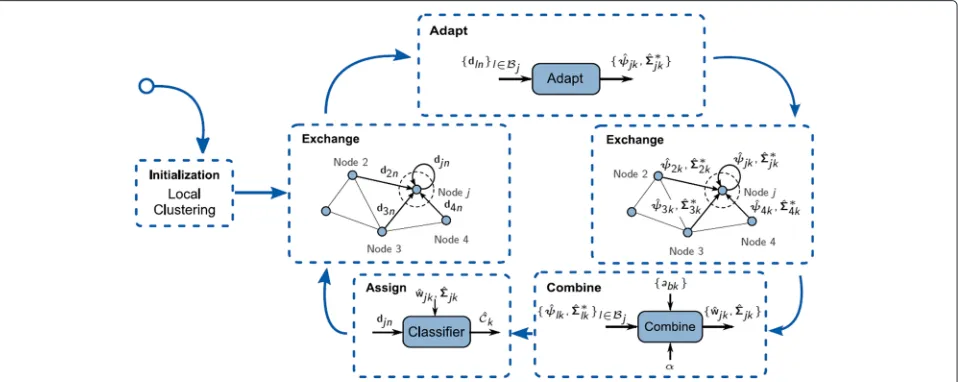
4.2 Communicationally Efficient Robust Distance-Based K-Medians Clustering/Classification over Adaptive Diffusion Networks (CE RDiff K-Med)
Since the RDiff K-Med may be demanding in terms of communication between sensors, which is a major con-tributor to the energy consumption of the devices [31], an algorithm is proposed which yields similar performance with reduced in-network communication: the “Commu-nicationally Efficient Robust Distance-Based K-Medians Clustering/Classification over Adaptive Diffusion Net-works” (CE RDiff K-Med).
The general procedure is similar to the RDiff K-Med except that there is no exchange of feature vectors between the nodes. The steps of theCE RDiff K-Medare the following:
1. Adaptation Step: Based on the feature vectors djn
stored inSjkn, each node calculates its intermediate
esti-matesψˆjknandˆ∗jknaccording to (9)–(13).
2. Exchange Step:Instead of broadcasting the entire fea-ture vectors, the nodes share only their estimates of the cluster centersψˆjknand the respective covariance matri-cesˆ∗jknwith their neighbors.
Table 1Summary of the RDiff K-Med algorithm Algorithm: RDiff K-Med
Local Clustering Phase
1. for the firstNtfeature vectors do
2. for allj=1,. . .,Jdo
3. perform K-medians according to (8)
4. calculatewˆ0jkandˆ0jkvia (9)-(13)
5. store classified data inS0jk
6. end for
7. for allj=1,. . .,Jdo
8. perform synchronization of cluster estimates
9. end for
10. for allj=1,. . .,Jdo
11. exchangeS0
jkwith all neighborsi∈Bj 12. store received data inV0jk
13. end for
14. end for
Distributed Classification Phase
15. forn=Nt,Nt+1, ..,Ndo
16. for allj=1,. . .,Jdo
17. broadcast an update forVjknto all neighbors
i∈Bj
18. end for
19. for allj=1,. . .,Jdo
20. determineψˆjknandˆ∗jknvia (9)-(13)
21. end for
22. for allj=1,. . .,Jdo
23. broadcastψˆjknandˆ∗jknto all neighborsi∈Bj
24. end for
25. for allj=1,. . .,Jdo
26. determinewˆjk(n)andˆjknvia (14) & (15) 27. calculate distances from feature vectordjnto all
ˆ
wjknby evaluating (17) or (18)
28. assigndjnto classCkwhich minimizes (17) or (18)
29. end for
30. end for
3. Combine Step:Each sensor jcombines its neighbor’s estimates analogously to (14) and (15) in order to obtain improved estimateswˆjknandˆjkn.
4. Classification Step: Based on the estimates deter-mined in the previous step, the distance measure of the feature vector to the estimates of the class centroids is evaluated and djn is classified analogously to the RDiff
Fig. 4Overview of the Communicationally Efficient Robust Distance-Based K-Medians Clustering/Classification over Adaptive Diffusion Networks (CE RDiff K-Med) algorithm
An overview of theCE RDiff K-Medalgorithm is pro-vided in Fig. 4, a summary is given in Table 2.
5 Numerical experiments
This section evaluates the performance of the proposed algorithm numerically in terms of the error rate in a broad range of conditions, i.e., different distributions of the outliers, different percentages of outliers in the feature vectors, different dimensions of the input data, different numbers of clusters and in terms of the adaptation speed in case of non-stationary data. Furthermore, the com-munication cost for different neighborhood sizes and the computation time as a function of the data dimension is considered. When reasonable, we compare our proposed method to the DKM [17].
5.1 Benchmark: distributed K-means (DKM)
As a benchmark, this paper considers theDistributed K-Means(DKM) algorithm by Forero et al., for details, see [17]. The basic idea of the DKM is to cluster the observa-tions into a given number of groups, such that the sum of squared-errors is minimized, that is
arg min wk,μpjnk
1 2
J
j=1 K
k=1 Nj
n=1
μp
jnkdjn−wk2, (19)
where wk is the cluster center for class k, μjnk ∈[ 0, 1]
is the membership coefficient of djn to class k, and
p ∈[ 1,+∞] is a tuning parameter. The DKM iteratively solves the surrogate augmented Lagrangian of a dis-tributed clustering problem based on (19) while exchang-ing the resultexchang-ing parameters among neighborexchang-ing nodes.
Although the DKM achieves very good performance in many scenarios, a major drawback is that the clustering is
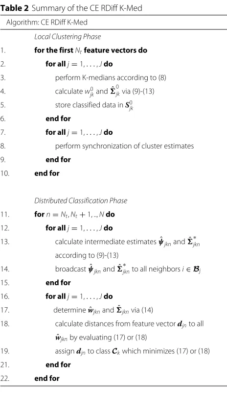
Table 2Summary of the CE RDiff K-Med Algorithm: CE RDiff K-Med
Local Clustering Phase
1. for the firstNtfeature vectors do
2. for allj=1,. . .,Jdo
3. perform K-medians according to (8)
4. calculatew0jkandˆ0jkvia (9)-(13)
5. store classified data inS0jk
6. end for
7. for allj=1,. . .,Jdo
8. perform synchronization of cluster estimates
9. end for
10. end for
Distributed Classification Phase
11. forn=Nt,Nt+1, ..,Ndo
12. for allj=1,. . .,Jdo
13. calculate intermediate estimatesψˆjknandˆ∗jkn
according to (9)-(13)
14. broadcastψˆjknandˆ∗jknto all neighborsi∈Bj
15. end for
16. for allj=1,. . .,Jdo
17. determinewˆjknandˆjknvia (14)
18. calculate distances from feature vectordjnto all
ˆ
wjknby evaluating (17) or (18)
19. assigndjnto classCkwhich minimizes (17) or (18)
21. end for
performed based on all available data and that it may need a high number of iterations until it converges to its final solution. This property makes the DKM difficult to use in real-time applications where an observation needs to be classified based on streaming data, such as for example in speaker labeling for MDMT speech enhancement [2] or object labeling in MDMT video enhancement for camera networks [9]. In addition to that, the performance of the DKM is limited in scenarios where feature vectors contain outliers.
5.2 Simulation setup
The simulations are based on a scenario with J = 10 nodes which are randomly distributed in space. Each node is connected to the four neighboring nodes which have the smallest Euclidean distance. Unless mentioned oth-erwise, classification is performed on K = 3 classes with centers w1 = (1, 1, 1)T, w2 = (1, 4, 3)T, w3 =
(3, 1, 1)T. Each sampledjnis drawn at random from class
kfrom the densityN(djn;wk,k)with covariance
matri-ces1 = (1, 0.01, 0.01)TI3,2 = (0.16, 4, 0.16)TI3and
3 = (0.25, 0.01, 4)TI3. Each node has NJ = 80
sam-ples available, 20 for the initialization and 60 for real-time classification. K-Medians is run three times, and the result which minimizes (8) is used for the classification. The parameters for the benchmark algorithm DKM are set p=ν=2, wherep=2 enables soft clustering andν=2 is the tuning parameter which yields the best results in the performance tests in [17]. The result is obtained having allNJ = 80 samples per node available. Since the
perfor-mance of the DKM depends on the number of iterations, we provide simulation results for multiple choices of the amount of iterations.
The generation of outliers considers a certain percent-age of samples to be replaced by a new sample which
is drawn from a contaminating distribution (Gaussian or chi-square). The error rate is calculated based on the classified samples excluding any outliers. The displayed results represent the averages that are based on 100 Monte-Carlo runs.
5.3 Simulation results
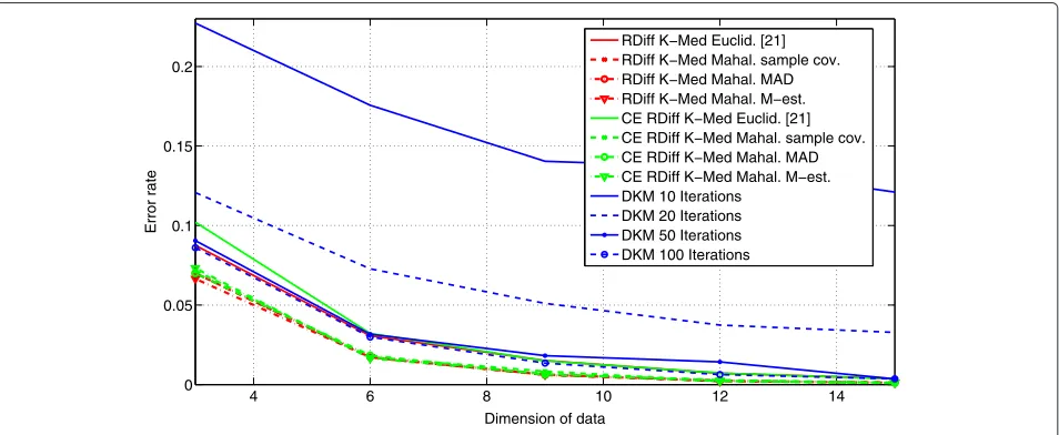
In Fig. 5, the impact of the dimension of the feature vectors on the performance is depicted. The data is generated by concatenating the mean values and covari-ance matrices until they have the according dimension. For example, w3 = (3, 1, 1)T is changed to w3 =
(3, 1, 1, 3, 1, 1)T and
3 = (0.25, 0.01, 4)TI3 becomes
3 = (0.25, 0.01, 4, 0.25, 0.01, 4)TI6 in order to obtain
data of dimensionq = 6 and so on. For increasing data dimension, the error rates for all considered algorithms decreases continuously.
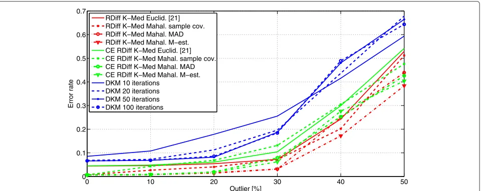
Figure 6 depicts the error rate of the algorithms under test as a function of the percentage of outliers in the data, where 0 % corresponds to the outlier free case. Here, the outliers are drawn at random from a Gaussian distribu-tion with the densityN((10, 10, 10)T,I3). The simulation
is run with the different estimators of covariance intro-duced in Section 3, the location is estimated using the median. The robust distance measures result in smaller error rates than the Euclidean distance.
Since in real-world scenarios, the outliers usually do not follow any specific distribution, the question arises how the algorithms deal with other types of outliers, e.g., from a skewed heavy tailed distribution. For the evaluation of this scenario, the outliers are now generated by a chi-square distribution with different degrees of freedomvfor each class: to a certain percentage of the feature vectors a vector is added which is drawn at random from a chi-square distribution where for each class, different values
4 6 8 10 12 14
0 0.05 0.1 0.15 0.2
Error rate
RDiff K−Med Euclid. [21] RDiff K−Med Mahal. sample cov. RDiff K−Med Mahal. MAD RDiff K−Med Mahal. M−est. CE RDiff K−Med Euclid. [21] CE RDiff K−Med Mahal. sample cov. CE RDiff K−Med Mahal. MAD CE RDiff K−Med Mahal. M−est. DKM 10 Iterations
DKM 20 Iterations DKM 50 Iterations DKM 100 Iterations
Dimension of data
0 10 20 30 40 50 0
0.1 0.2 0.3 0.4 0.5 0.6
Outlier [%]
Error Rate
RDiff K−Med Euclid. [21] RDiff K−Med Mahal. sample cov. RDiff K−Med Mahal. MAD RDiff K−Med Mahal. M−est. CE RDiff K−Med Euclid. [21] CE RDiff K−Med Mahal. sample cov. CE RDiff K−Med Mahal. MAD CE RDiff K−Med Mahal. M−esti. DKM 10 iterations
DKM 20 iterations DKM 50 iterations DKM 100 iterations
Fig. 6Average error rate for different estimators of covariance as a function of the amount of outliers from a Gaussian distribution with the density N((10, 10, 10)T,I
3)
forvare chosen. This is done in order to create a non-symmetric outlier distribution instead of a constant shift of the mean of the outlier distribution for all classes. In this manner, for the first classC1, a randomly drawn vector
of dimensionqwithv1=3 is added to a certain number of
data vectors, a vector withv2=5 is subtracted from
cor-responding feature vectors of classC2and forC3a different
random number is drawn for each direction in space: gen-erated withv3,1 = 4,v3,2 = 1 andv3,3 = 7 forx,yand
zdirection, respectively, whereby v3,2 = 1 is subtracted
from they-component. For this simulation, a scenario is chosen with more distinct clusters with centroidsw1 =
(1, 1, 1)T, w
2 = (0, 5, 3)T, w3 = (3, 3, 7)T. The result is
given in Fig. 7.
Figure 8 shows the error performance as a function of the number of feature vectors which are available per node. Both the DKM fori=10 andi= 20 and the RDiff K-Med and CE RDiff K-Med with robust estimation meth-ods show a slightly decreasing error rate with a growing number of feature vectors.
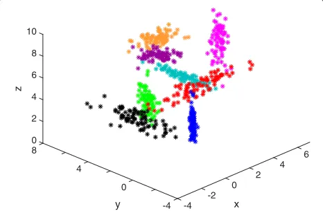
For the next experiment, we evaluate a more complex scenario consisting of eight clusters of different shapes and sizes distributed in space (see Fig. 9). The cen-troids are chosen as w1 = (1, 0, 3)T, w2 = (1, 4, 3)T,
0 10 20 30 40 50
0 0.1 0.2 0.3 0.4 0.5 0.6 0.7
Outlier [%]
Error rate
RDiff K−Med Euclid. [21] RDiff K−Med Mahal. sample cov. RDiff K−Med Mahal. MAD RDiff K−Med Mahal. M−est. CE RDiff K−Med Euclid. [21] CE RDiff K−Med Mahal. sample cov. CE RDiff K−Med Mahal. MAD CE RDiff K−Med Mahal. M−est. DKM 10 iterations
DKM 20 iterations DKM 50 iterations DKM 100 iterations
10 20 30 40 50 60 70 80 90 100 0
0.05 0.1 0.15 0.2 0.25 0.3
Number of feature vectors per node
Error rate
RDiff K−Med Euclid. [21] RDiff K−Med Mahal. sample cov RDiff K−Med Mahal. MAD RDiff K−Med Mahal. M−est. CE RDiff K−Med Euclid. [21] CE RDiff K−Med Mahal. sample cov. CE RDiff K−Med Mahal. MAD CE RDiff K−Med Mahal. M−est. DKM 10 Iterations
DKM 20 Iterations DKM 50 Iterations DKM 100 Iterations
Fig. 8Error rate as a function of the available number of feature vectors per node
w3 = (1, 0, 6)T, w4 = (−1, 3, 3)T, w5 = (4, 4, 4)T, w6 = (6, 3, 7)T, w7 = (4.5, 7, 6)T and w8 =
(2, 4, 7)T with corresponding covariance matrices1 =
(0.1, 0.1, 1)TI3,2=(0.1, 0.4, 1)TI3,3=(2, 0.1, 0.5)TI3,
4 = (0.4, 1.6, 0.4)TI3, 5 = (0.2, 1.2, 0.1)TI3,
6 = (0.25, 0.3, 1.5)TI3, 7 = (0.8, 0.5, 0.2)TI3 and
8 = (0.5, 0.5, 0.3)TI3. The outliers are drawn
ran-domly from a Gaussian distribution with the density N((10, 10, 10)T,I
3). The results are provided in Fig. 10.
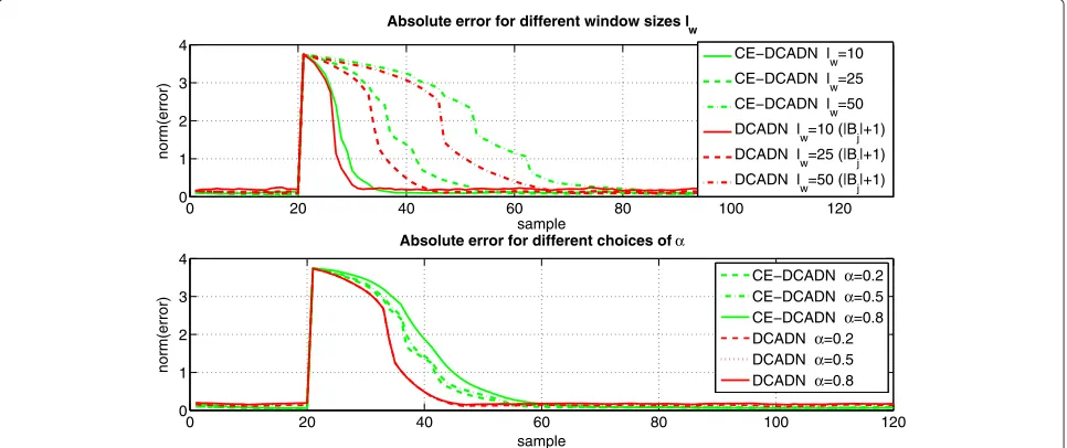
The former performance studies were based on the assumption that the data is stationary. Next, it is examined how the proposed algorithms perform for non-stationary feature vectors. For this purpose the value of a single con-sidered cluster centroid is instantly changed during the classification process. The adaptation speed of the RDiff K-Med and the CE RDiff K-Med is examined for different window sizeslwand different values forα (see Eqs. (14)
and (15)) by calculating the error which is given by the
6 4 2
x 0 -2 -4 -4 0
y 4 8 0 10
2 4 8
6
z
Fig. 9Scenario with eight clusters of different shapes and sizes
norm of the difference between the true value and the estimate of the cluster centroid. Unlike the CE RDiff K-Med the RDiff K-K-Med stores not only its own feature vec-tors, but also the feature vectors from its neighborhood, it has(|Bj| +1)data vectors per time step available instead
of only one. In order to make the window sizes for both algorithms comparable,lwis chosen such that it contains
the feature vectors oflwtime steps. As a consequence, the
compared window length of the RDiff K-Med corresponds to (| Bj | +1)times the window length of the CE RDiff
K-Med. The result is shown in Fig. 11. As depicted in the upper plot, a large window size results in a slower adap-tation speed. The RDiff K-Med adapts faster to the true cluster centroid than the CE RDiff K-Med since its esti-mation is based on more available samples. However, the CE RDiff K-Med yields a smaller error compared to the RDiff K-Med when both have adapted to the true value. The choice of the factorα(see lower plot) has no signifi-cant impact on the RDiff K-Med. For the CE RDiff K-Med a smaller value forα(and therefore a higher weighting of the estimates of the neighboring nodes) leads to a higher adaptation speed. Since it has only a small amount of fea-ture vectors available, this method is dependent on the data exchange with its neighbors.
5.4 Communication cost and computation time
0 10 20 30 40 50 0
0.05 0.1 0.15 0.2 0.25 0.3 0.35
Outlier [%]
Error Rate
RDiff K−Med Euclid. [21] RDiff K−Med Mahal. sample cov RDiff K−Med Mahal. MAD RDiff K−Med Mahal. M−est. CE RDiff K−Med Euclid. [21] CE RDiff K−Med Mahal. sample cov. CE RDiff K−Med Mahal. MAD CE RDiff K−Med Mahal. M−est. DKM 10 Iterations
DKM 20 Iterations DKM 50 Iterations DKM 100 Iterations
Fig. 10Average error rate for different estimators of covariance as a function of the amount of outliers from a Gaussian distribution with the density N((10, 10, 10)T,I
3)
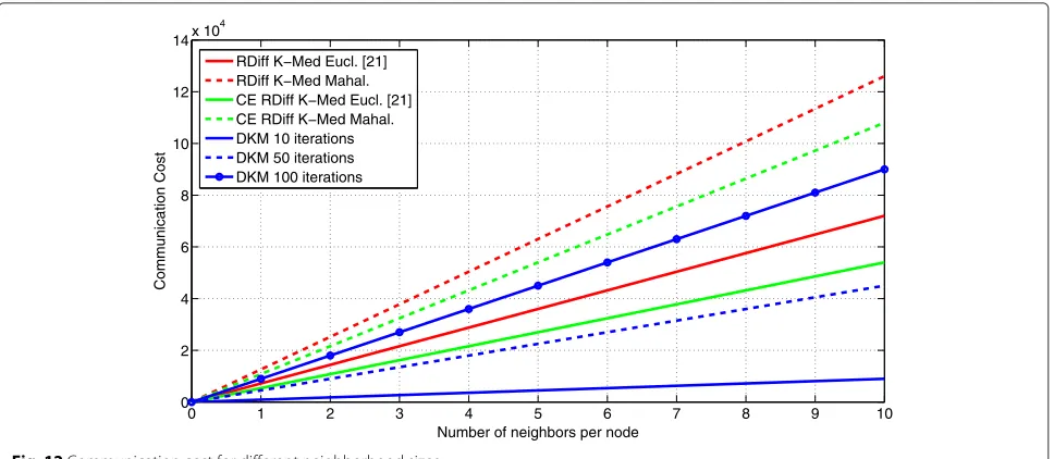
each node. The communication cost displayed in Fig. 12 is specified in data units, where one matrix entry forms one unit. It becomes clear that the choice of the neighborhood size has a high impact on the communication costs. For the DKM the number of iterations is crucial. While for a small amount of clusters few iterations may be sufficient, the number of iterations that is necessary for a good per-formance increases for higher cluster numbers (see [17] for more detailed information) which results in strongly increasing communication costs.
The computation time as a function of the dimension of the data is provided by Fig. 13 and given in seconds (using an Intel Core i7 5820K). Whereas the DKM has a constant computation time independent of the data dimension, it increases with the data dimension for the proposed algorithms. The resulting computation time for using the M-estimator is notably higher than for the other approaches which makes it hardly real-time capable. The other estimation methods take equally long for each algo-rithm while the CE RDiff K-Med has a much shorter
0 20 40 60 80 100 120
0 1 2 3 4
sample
norm(error)
Absolute error for different window sizes l w
CE−DCADN l w=10 CE−DCADN l
w=25 CE−DCADN l
w=50 DCADN l
w=10 (|Bj|+1) DCADN l
w=25 (|Bj|+1) DCADN l
w=50 (|Bj|+1)
0 20 40 60 80 100 120
0 1 2 3 4
sample
norm(error)
Absolute error for different choices of α
CE−DCADN α=0.2 CE−DCADN α=0.5 CE−DCADN α=0.8 DCADN α=0.2 DCADN α=0.5 DCADN α=0.8
0 1 2 3 4 5 6 7 8 9 10 0
2 4 6 8 10 12 14x 10
4
Number of neighbors per node
Communication Cost
RDiff K−Med Eucl. [21] RDiff K−Med Mahal. CE RDiff K−Med Eucl. [21] CE RDiff K−Med Mahal. DKM 10 iterations DKM 50 iterations DKM 100 iterations
Fig. 12Communication cost for different neighborhood sizes
computation time due to the smaller data sets it has to work with.
6 Conclusions
Two generic robust diffusion-based distributed hybrid classification algorithms were proposed, which can be adapted to various object/source labeling applications in a decentralized MDMT network. A performance compari-son to the DKM was provided and the proposed methods showed promising results. Even in direct comparison with the DKM which permanently has access to all available samples, since it is operating in batch mode, our pro-posed online methods provide comparable error rates to the DKM using 50 iterations and more. Unlike the DKM,
both the RDiff K-Med and CE RDiff K-Med are potentially real-time capable.
The choice of the distance metric has a considerable impact on the performance of the proposed classification algorithms. Using the Mahalanobis distance yields sig-nificantly smaller error rates compared to the Euclidean distance while resulting in higher communication costs and computation time.
Future work will include the application of this algorithm to real-world speech source labeling, object labeling in camera networks as well as labeling of semantic information based on occupancy grid maps for autonomous mapping and navigation with multiple rescue robots [32].
4 6 8 10 12 14
100 101 102 103 104
Data dimension
Computation time
RDiff K−Med Euclid. [21] RDiff K−Med Mahal. MAD RDiff K−Med Mahal. M−est. CE RDiff K−Med Euclid. [21] CE RDiff K−Med Mahal. MAD CE RDiff K−Med Mahal. M−est. DKM 10 Iterations
DKM 50 Iterations DKM 100 Iterations
Competing interests
The authors declare that they have no competing interests.
Acknowledgements
This work of P. Binder was supported by the LOEWE initiative (Hessen, Germany) within the NICER project and by the German Research Foundation (DFG). The work of M. Muma was supported by the Future and Emerging Technologies (FET) programme within the Seventh Framework Programme for Research of the European Commission (HANDiCAMS), under FET-Open grant number: 323944.
Received: 6 August 2015 Accepted: 26 February 2016
References
1. E Hänsler,Statistische Signale: Grundlagen und Anwendungen. (Springer, Berlin, 2013)
2. A Bertrand, M Moonen, Distributed signal estimation in sensor networks where nodes have different interests. Signal Process.92(7), 1679–1690 (2012)
3. N Bogdanovic, J Plata-Chaves, K Berberidis, Distributed
incremental-based LMS for node-specific adaptive parameter estimation. IEEE Trans. Signal Process.62(20), 5382–5397 (2014)
4. J Plata-Chaves, A Bertrand, M Moonen, inAcoustics, Speech and Signal Processing (ICASSP), 2015 IEEE Int. Conf. on. Distributed signal estimation in a wireless sensor network with partially overlapping node-specific interests or source observability, (2015), pp. 5808-5812
5. J Chen, C Richard, AH Sayed, Diffusion LMS over multitask networks. IEEE Trans. Signal Process.63(11), 2733–2748 (2015)
6. J Chen, C Richard, AH Sayed, Multitask diffusion adaptation over networks. IEEE Trans. Signal Process.62(16), 4129–4144 (2014)
7. E Hänsler, G Schmidt,Speech and Audio Processing in Adverse Environments. (Springer, Berlin, 2008)
8. S Chouvardas, M Muma, K Hamaidi, S Theodoridis, AM Zoubir, inProc. 40th IEEE Int. Conf. Acoustics, Speech and Signal Processing (ICASSP). Distributed robust labeling of audio sources in heterogeneous wireless sensor networks, (2015), pp. 5783–5787
9. FK Teklehaymanot, M Muma, B Béjar-Haro, P Binder, AM Zoubir, M Vetterli, inProc. 12th IEEE AFRICON (accepted). Robust diffusion-based
unsupervised object labelling in distributed camera networks, (2015) 10. A D’Costa, A Sayeed, inIEEE Military Communications Conference
(MILCOM). Data versus decision fusion for distributed classification in sensor networks, vol. 1, (2003), pp. 585–5901
11. D Li, KD Wong, YH Hu, AM Sayeed, Detection, classification and tracking of targets in distributed sensor networks. Technical report, Department of Electrical and Computer Engineering, University of Wisconsin-Madison, USA 12. F Fagnani, S Fosson, C Ravazzi, A distributed classification/estimation
algorithm for sensor networks. SIAM J Control Optim.52(1), 189–218 (2014)
13. M Hai, S Zhang, L Zhu, Y Wang, inInd. Control and Electron. Eng. (ICICEE), 2012 Int. Conf. On. A survey of distributed clustering algorithms, (2012), pp. 1142–1145
14. E Kokiopoulou, P Frossard, Distributed classification of multiple observation sets by consensus. IEEE Trans. Signal Process.59(1), 104–114 (2011)
15. B Malhotra, I Nikolaidis, J Harms, Distributed classification of acoustic targets in wireless audio-sensor networks. Comput. Netw.52(13), 2582–2593 (2008)
16. RD Nowak, Distributed em algorithms for density estimation and clustering in sensor networks. IEEE Trans. Signal Process.51(8), 2245–2253 (2003)
17. P Forero, A Cano, GB Giannakis, et al., Distributed clustering using wireless sensor networks. IEEE J. Sel. Topics Signal Process.5(4), 707–724 (2011) 18. S-Y Tu, AH Sayed, Distributed decision-making over adaptive networks.
IEEE Trans. Signal Process.62(5), 1054–1069 (2014)
19. D Wang, J Li, Y Zhou, inIEEE/SP 15th Workshop on Stat. Signal Process. (SSP). Support vector machine for distributed classification: a dynamic consensus approach, (2009), pp. 753–756
20. X Zhao, AH Sayed, Distributed clustering and learning over networks. IEEE Trans. Signal Process.63(13), 3285–3300 (2015)
21. P Binder, M Muma, AM Zoubir, inProc. 40th IEEE Int. Conf. Acoustics, Speech and Signal Processing (ICASSP). Robust and computationally efficient diffusion-based classification in distributed networks, (Brisbane, Australia, 2015), pp. 3432–3436
22. X Zhao, AH Sayed, inProc. International Workshop on Cognitive Information Processing (CIP). Clustering via diffusion adaptation over networks, (2012), pp. 1–6
23. AH Sayed, Adaptation, learning, and optimization over networks. Found. Trends Mach. Learn.7(4-5), 311–801 (2014)
24. S Khawatmi, AM Zoubir, AH Sayed, inProc. 23rd European Signal Processing Conf. (EUSIPCO). Nice, France. Decentralized clustering over adaptive networks, (Nice, France, 2015), pp. 2745–2749
25. AH Sayed, Adaptive networks. Proc. IEEE.102(4), 460–497 (2014) 26. AM Zoubir, V Koivunen, Y Chakhchoukh, M Muma, Robust estimation in
signal processing: a tutorial-style treatment of fundamental concepts. Signal Process. Mag. IEEE.29(4), 61–80 (2012)
27. PA Forero, V Kekatos, GB Giannakis, Robust clustering using outlier-sparsity regularization. IEEE Trans. Signal Process.60(8), 4163–4177 (2012) 28. R Maronna, D Martin, V Yohai,Robust Statistics. (John Wiley & Sons,
Chichester, 2006)
29. PJ Huber, et al., Robust estimation of a location parameter. Ann. Math. Stat.35(1), 73–101 (1964)
30. FS Cattivelli, AH Sayed, Diffusion LMS strategies for distributed estimation. IEEE Trans. Signal Process.58(3), 1035–1048 (2010)
31. D Estrin, L Girod, G Pottie, M Srivastava, inIEEE Int. Conf. Acoustics, Speech and Signal Processing (ICASSP). Instrumenting the world with wireless sensor networks, vol. 4, (2001), pp. 2033–2036
32. S Kohlbrecher, J Meyer, T Graber, K Petersen, U Klingauf, O von Stryk, in RoboCup 2013: Robot World Cup XVII. Hector open source modules for autonomous mapping and navigation with rescue robots (Springer, Berlin, 2014), pp. 624–631
Submit your manuscript to a
journal and benefi t from:
7Convenient online submission
7Rigorous peer review
7Immediate publication on acceptance
7Open access: articles freely available online
7High visibility within the fi eld
7Retaining the copyright to your article