Mesh Simplification Using the Edge Attributes
Il Dong Yun
School of Electronics and Information Engineering, Hankuk University of F. S., Yongin 449-791, Korea Email: [email protected]
Kyowoong Choo
Motorola Korea Design Center, Seoul 135-766, Korea Email: [email protected]
Sang Uk Lee
School of Electrical Engineering, Seoul National University, Seoul 151-742, Korea Email: [email protected]
Received 14 November 2001 and in revised form 15 February 2002
This paper presents a novel technique for simplifying a triangulated surface at different levels of resolution. While most existing algorithms, based on iterative vertex decimation, employ the distance for error metric, the proposed algorithm utilizes an edge criterion for removing a vertex. Aninterior angleof a vertex is defined as the maximum value of all possible angles formed by combinations of edges connected to a vertex. Since the surface curvature examined with the interior angle provides more information for decision of vertex removal than the conventional distance measure, the proposed algorithm can approximate the surface with less computation. The height of a triangle, which is formed by the pair of edges, is also used for an additional constraint. The computational complexity can thus be greatly alleviated to logarithmic scale from the exponential scale required for the conventional algorithms, while yielding the comparable error level.
Keywords and phrases:LOD, level of detail, mesh simplification, multiresolution.
1. INTRODUCTION
Detailed mesh data models, obtained from range scanning systems, are too dense for practical applications. Transmis-sion and storage requirements of such 3D graphic models are very demanding, due to the large amounts of data [1]. While rendering performance is continually improving, further im-provement in performance could be possible by adapting the complexity of a model to its contribution to the rendered im-age. The ideal solution will efficiently determine the coarsest model, while retaining the perceptual image qualities.
One common heuristic technique is to author several ver-sions of a model at variouslevel of detail(LOD); a detailed triangle mesh is used when the object is close to the viewer, and coarser approximations are substituted as the viewing distance increases. The LOD assigns multiple models vary-ing in resolution for an object. Thus, virtual reality (VR) ma-chines can render objects in a virtual world according to their proper resolution, without displaying all the polygons in full detail.
The multiresolution modeling, motivated by such re-quirements, approximates high-density models nearly indis-tinguishably with fewer faces for rendering efficiency [2].
This is accomplished by iteratively removing vertices from original faces that will not significantly degrade the global shape of the model. The distance from the original surface to the reformed one usually represents the error caused by removing each vertex. Most existing algorithms mainly dif-fer in theirorderof choosing a vertex for removal. However, heavy computation is required for estimating the consequen-tial errors caused by removing a vertex. These approaches cannot provide much information about the surface, while they can be implemented easily. Edge contraction as well as vertex decimation, to be introduced in Section 2, falls into this category. Edge contraction collapsing vertices, lying on both sides of an edge, lacks diversity in the simplification of a given region, because pulling both ends of an edge to the middle is the only required operation.
the surface curvature of adjacent triangles are evaluated and sorted to collapse the centering triangle’s three vertices to a single point, all regions connected are affected, resulting in significant variations in surface structure.
The edge, on the other hand, contains enough—if not complete—information about the local surface surrounding a vertex, while keeping the variation small. The surface in-formation can be easily obtained by evaluating the interior angles of the surrounding edges. Hence, by adopting an edge as a primitive, a vertex to be removed can be selected quickly, reflecting the surface information as well. While the exist-ing algorithms consume much time in whether or not to move a vertex by actually removing and evaluating the re-sulting error, the proposed approach works deterministically by removing vertices in the order of their height and angle without further analysis. In addition, by filling the hole with Delaunay triangulation, we can give more degree of freedom than the conventional edge collapse approaches in the retri-angulation of simplified area. Therefore, both the computa-tional load and surface estimation errors can be reduced by utilizing the edge information.
2. PREVIOUS APPROACHES IN MESH SIMPLIFICATION
The approaches to be introduced are minimum number vertex-based approximations. For this kind of the approx-imation problem, we consider the given error bound . Then the objective is to minimize the number of vertices such that no point of the approximation is further away than from the input model [4]. As will be discussed in Section 2.1, most approaches rely solely on the vertex er-ror with perhaps one or more additional constraints. This can only give obscure information about the surface to be approximated, yielding to a simplified object whose errors are minimum in numeric domain only, which is not visually optimum.
2.1. Vertex decimation
Vertex decimation is an iterative surface simplification ap-proach [5, 6, 7]. In each step, when a vertex is selected for removal, all faces adjacent to that vertex are removed from the model, then the resulting hole is retriangulated. Because the main purpose of these algorithms is to reduce the den-sity of acquired meshes, we should be careful to preserve the topology.
One of the first iterative mesh simplification algorithms was proposed by Lorensen et al. [5], in which the vertices are removed from the mesh, and the local neighborhood sur-rounding the point is retriangulated on the local plane of the vertex. A point is removed when the distance to the best-fit plane of the surrounding point is small. All vertices with an error that is less than a threshold and satisfying topology pre-serving condition, are removed. Since primitives are not or-dered for decimation, a vertex with greater error may be re-moved first.
Soucy and Laurendeau [6, 7] presented a sequential op-timization algorithm, in order to remove the vertex that minimizes the retriangulation error after each iteration. The
Edge collapse Vertex decimation
Figure1: Comparison of freedom of retriangulation between edge collapse and vertex decimation.
purpose of the sequential algorithm is to remove the maxi-mum number of vertices, while keeping the triangulation er-ror as low as possible. The equi-angularity of surface trian-gulation is optimized in 3D space throughout the sequential process, by using an unconstrained Delaunay triangulation algorithm [8]. The main disadvantage of these algorithms, however, is that the cost of computation is very expensive. Since it needs to evaluate all errors from previously removed vertices, the computational complexity increases as the pro-cess goes on. In general, the computation is proportional to the exponential scale.
2.2. Edge contraction
An edge contraction takes two endpoints of a target edge, moves them to the same position, links all the incident edges to one of the vertices, deletes the other vertex, and removes any faces that have degenerated into lines or points. These algorithms iteratively contract the edges of the model. The primary difference lies inhowto choose the particular edge to be collapsed [9, 10, 11].
Gu´eziec’s [9] mesh simplification algorithm improves Schroeder’s algorithm in many ways. Gu´eziec employs edges as the mesh primitive and edge collapse to eliminate retrian-gulation from the mesh simplification algorithm. The edges are ordered based on edge length, and a single pass through the edges is performed. During edge collapse, a new vertex is created. As in most approaches, Gu´eziec’s simplification method bounds the total change in mesh shape. However, mesh shape is bounded using a complex construction called a tolerance volume, whose update requires a dynamic pro-gramming approach. Furthermore, Gu´eziec’s algorithm can-not explicitly control the resolution of the generated meshes and cannot handle the vertices along the boundary of a mesh to prevent shrinking during simplification.
the degree of freedom for retriangulation between edge con-traction and vertex decimation approaches.
2.3. Remarks
This section presents several vertex-based multiresolution modeling techniques, each of which has its own input cri-teria and advantages or disadvantages. The vertex-based al-gorithm is mainly based on vertex decimation and edge con-traction approaches. Both evaluate the resulting error (or en-ergy functions) caused by removing each vertex, then de-cide whether or not to allow the decimation (contraction). This error estimation should be repeated after each iteration, making it computationally expensive.
In addition, a face-based approach, utilizing the surface curvature between adjacent triangles, is not adequate for pre-serving topology, since it affects unnecessary larger area, in order to preserve the triangular structure. In this paper, an attempt is made to utilize both the curvature and the dis-tance (error) information, while preserving the topology and yielding small numerical errors.
3. EDGE-BASED MESH SIMPLIFICATION
Our main aim is confined to vertex decimation-based mul-tiresolution modeling, on the notion that vertex decimation guarantees zero error on remaining vertices, because it does not move vertices’ position. Among the well-known vertex decimation-based algorithms, Soucy’s vertex removal algo-rithm could be one of the best approaches, since the result-ing error by removresult-ing a vertex is re-calculated and sorted after each iteration. Although Soucy’s method seems to be reasonable at each step, it also cannot provide the global op-timal solution for removing a given number of vertices for minimum error. In addition, the computational complexity is very expensive, since the error evaluation is required for every iteration.
Soucy’s approach can be classified as the distance-based vertex removal. However, the distance itself may not be a good primitive for curvature estimation in surface simpli-fication. The proposed approach is based on simple notion that high curvature regions are preserved and low curvature regions simplified. Therefore, by using both curvature and distance as primitives, better results could be expected.
3.1. Edge-based vertex removal algorithm
The proposed edge-based vertex removal algorithm utilizes curvature and distance information for evaluating the se-quence of reduction. An angle between adjacent edges pro-vides an approximate curvature of the surface lying on that edge pair. Aninterior angleof a vertex is defined as the maxi-mum value of all possible angles between edges connected to a vertex.
In Figure 2a, a vertex in the center is connected by six neighboring vertices to form a hexagon when seen from above. If the interior angle between a pair of edges is close to 180◦, it can be assumed that this pair may not distort the global shape significantly, when substituted by a single
(a) Original edge pair. (b) Merged edge pair.
Figure2: Removal of a vertex lying on a semi-straight edge pair.
180
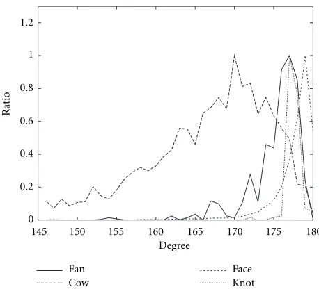
Figure3: Histogram of interior angles.
edge. Hence, the vertex in the center qualifies to be in the queue of removal. Figure 2b shows the vertex removing and re-meshing by Delaunay triangulation. In this case, a pair of edges whose angle is close to 180◦is replaced by a single edge drawn in thick line, then re-meshing procedure is performed on both sides of the edge. In order to justify the assumption, in our approach, the statistics of theinterior angle distribu-tion of the following 3D data are considered.
(i) The Fan, Face, and Knot data which are acquired from the STL objects library at ftp://fantasia.eng.clemenson.edu/ SLA/STL objects.
(ii) The Cow data which was acquired from http:// almond.srv.cs.cmu.edu/afs/cs/user/garland.
Figure4: Initial triangulation of a dense range data.
However, the proposed algorithm includes a retriangu-lation process that may not preserve the surface contour of original model when applied inappropriately. Fortunately, the merged edge prevents this variation by constraining the area of retriangulation. While the previous algorithms retri-angulates the whole area of vertex decimation, the proposed algorithm divides the area by two with the merged edge ly-ing across it, constrainly-ing the region of retriangulation into smaller parts. Detailed description is presented in the follow-ing subsection.
There would be many retriangulation solutions, depend-ing on the number of edges linked with the vertex. In ad-vance, it is necessary to examine the distribution of edge numbers connected to a vertex. Normally, a dense range data, acquired from laser scanners, usually form a regular grid structure. The surface triangles can be easily made, by sim-ply connecting vertices in horizontal and vertical directions to form a quadrangle, and by adding a diagonal line to di-vide this quadrangle into a triangle. An example is illustrated in Figure 4. Thus, it is easy to show that a vertex on a reg-ular grid have six adjacent vertices connected by an edge. Experimentally obtained distribution of a connected num-ber of edges agrees to our expectation. The numnum-ber of con-nection exhibits a Gaussian-like distribution with mean≈6 as shown in Figure 5.
3.2. Edge-constrained retriangulation process
In large, the retriangulation process consists of two steps, de-pending on the adjacency of edge pair. The first is when the pair is not adjacent, and the other is when the edges are right next to each other. We begin with the adjacent pair, provid-ing Figure 6 for visual demonstration of the followprovid-ing de-scriptions. The adjacent pair drawn in thick lines in Figures 6b, 6d, and 6e shall be merged into an outer boundary edge, which is referred to as a boundary condition, denoted by “b.” The boundary condition occurs quite often, due to the recur-sive nature of the proposed approach. The problem of how the holes in Figures 6b, 6d, and 6e should be re-meshed by triangles is intensively studied by [7]. The main approach is filling the hole with Delaunay triangles which contains the most equi-angular set of triangles [12]. This criterion avoids long narrow triangles that are numerically unstable. A sim-ple algorithm introduced by Sibson [8] iteratively searches for adjacent triangles and swaps the diagonal (common edge) eventually converging to a Delaunay triangulation of the data points. Here, we use the interior angles of the triangles in 3D
10 8
6 4
2
Connected number of edges 0
Figure5: Histogram of edges linked to a vertex.
space as a metric for equi-angularity test, which is referred to as 212D triangulation [6].
The nonboundary conditions are the dominating events in the retriangulation process. Figure 6f of “Case 6” is a good example of the nonboundary condition. When the centroid is removed and the thick edge pair is substituted by a sin-gle edge, two areas remain to be retriangulated, which is sent recursively back to “Case 4b,” respectively. Then, “Case 4b” retriangulates each region with iterative edge swapping oper-ation of Sibson’s. In Figure 6a, “Case 3” is actually a special case where the elimination of the centroid does not depend upon the angle, because there is no angle to compare with. Since we have focused the proposed algorithm with an addi-tional distance criterion described in Section 3.3, no further manipulation of data is necessary, except for the deletion of the centroid from data list.
3.3. Enhancement with additional constraint
The approach discussed in Section 3.2 might not provide the satisfying results, because the proposed approach solely fo-cuses on fast algorithm for vertex removal. However, it is worthy to note that there are long edges still abundant in the reduced model. Thus, a criterion to reduce the long edges should be considered to enhance the overall performance. We consider a height parameterδ for the angle criterion when the interior angles are pre-calculated. As depicted in Figure 7, the height parameter is the height of a triangle made of two points at the end of each edge and the vertex in the center. As mentioned previously, “Case 3” is merged if the distance from the vertex to the surrounding triangle is less than the thresholdδ.
(a) Case 3. (b) Case 3b.
3b 3b
(c) Case 4. (d) Case 4b.
(e) Case 5b.
4b 4b
(f) Case 6.
Figure6: Classification of the retriangulation process.
(a) (b)
Figure7: Additional height constraintδ.
increases the heightλfrom 0 toδ, while the inner loop de-creases the angle θ from 180◦ to θmin. Thus, an edge pair with larger interior angle, has a priority when two or more edge pairs exist having the same height. When the minimum value (θmin) of the inner loop is set to zero, small eruptions on the surface may be deleted. This is absolutely normal in global curvature sense, since small eruptions on a surface will not be seen from a distance. However, to preserve these fea-tures, we only need to increaseθminin the inner loop from zero to higher value. The experiments show empirically that
θmin=150◦is sufficient for this purpose.
Swapping the outer and inner loops in the proposed al-gorithm may seem interesting. This can be reduced to the fundamental question of whether an edge pair with large in-terior angle has priority over the other edge pair which has the same height λ, but has smaller interior angle. It is con-cluded that the problem should be examined over the area affected by removal. Removal of pair with larger interior an-gle will have greater effect on neighboring regions which is undesirable in mesh simplification. Therefore, the swapping of loops is excluded from consideration.
3.4. Synthesis
The whole process is summarized in Figure 8. As the data is loaded, where the height thresholdδ, interior angleθ and height parameter λare set to 180◦ and 0, respectively. The outer loop increasesλfrom zero toδ, while the inner loop decreasesθfrom 180◦toθmin, which is chosen to be 150◦in the experiments. After the inner loop has completed search-ing and removsearch-ing vertices by decreassearch-ingθ, it is reset to 180◦ andλ is increased by adding previously defined∆λ = δ/k
Angle−−
Y Searched whole data?
N
N Display data
Store data Evaluate total error
Meets height & angle condition?
Y
Merge edges Retriangulation Pick vertex
Y Angle>0
N
Height++ Angle=180 Y
Height<max N
max=input threshold Angle=180
Height=0 Load data
Figure8: Block diagram for the proposed algorithm.
3.5. Computation of error
An error of decimated vertex is defined as its minimum dis-tance to the newly created surface. Since the proposed algo-rithm does not move vertices’ position, we only need to eval-uate the errors caused by removing the vertices. Two error metrics, that is,L∞andL2are widely used to evaluate the per-formance. TheL2error norm is the root mean square (RMS) error, while theL∞norm yields the maximum error bound. Both errors, defined by (1), are obtained for further analy-sis, whereNandnare the original and removed numbers of vertices, respectively. Usually, the percentage of error to the diagonal length of original model’s bounding box is used as a metric for comparison.
L2=
2
1+22+· · ·+n2
N , L∞ =
n
max
k=1 k. (1)
3.6. Time complexity of the proposed algorithm
Computational complexity mainly depends on the size of the data, because one of the bottle neck of the algorithm is the memory copying operations. When a vertex to be removed is found, all associated edges and triangles should be removed from its linked list. We simply generate a small temporary list for each, by copying the remaining edges and triangles, then swap the temporary list with the original one. Almost equal time is required when the hole is retriangulated to add edges and triangles to the linked list. The computational complex-ity could be alleviated, if this deletion process is optimized by dynamicallyallocating (deleting) spaces for the data. There-fore, the computational complexity is mainly dependent on (a) searching and (b) retriangulation process.
when a linked-list of lengthk has only one data that suites one’s need, the average searching time,skto find the suitable vertex is proportional to (k+ 1)/2, given by
sk∝ 1 + 2 +k· · ·+k =k+ 12 . (2)
Retriangulation process requires for deletion and addi-tion of triangles and edges. In average, when a vertex with six edges are deleted, which is the most popular case as shown in Figure 3, the required operations are (a) deletion of six trian-gles and six edges, and (b) addition of four new triantrian-gles and three new edges. Since removing or adding a triangle from a list of lengthlrequires 2(l−1) address copying operations, and the number of triangles and edges are proportional to the number of vertices by Euler’s formula, the time required for deletion and addition of triangle is proportional to the vertex list of lengthk, given by
rk∝
The first term is time for deletion of edges and triangles, respectively, while the second term is time for addition. The total time required for removingnvertices from an original model withNvertices is given by
Tn
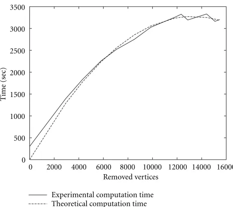
wherec1andc2are scaling constants. Note that the constants would depend on the computing performance and program-ming efficiency. To show the validity of the time complexity analysis, we compare the experimental and theoretical com-putation time for the Face model in Figure 9. The scaling constants are found to bec1 = −0.05302 andc2 =0.00069, respectively, by the least mean square curve fitting method.
4. EXPERIMENTS AND DISCUSSIONS
We implement the proposed algorithm on Windows NT Server 4.0 with Pentium II 400 MHz processor and 192 MB memory. The results areflat shaded, in order to exaggerate the distinction of triangles. The Fan model in Figure 10 is a typical model produced by a CAD tool. The vertices and edges are almost optimally placed, which is almost impossi-ble by actual modeling via range scanners. The original wire-frame model is back-face culled in order to emphasize the placements of primitives. The simplification process faith-fully preserves the unique characteristics of Fan’s hole and wings. The result consists of only 19% of the original data, with tolerable errors provided in Table 1.
Figure 11 shows the hierarchy of Cow models from high to low resolution. The histogram indicates that vertices with high interior angles are mostly removed during the iteration. High curvature regions such as horn, ear, and nipples are well
16000
Figure9: Time consumed for Face model of 16374 vertices.
Table1: Summary of results on Fan model.
δ No. of triangles L2error (%) L∞error (%) Data ratio (%)
0 2750 0 0 100
2.0 1978 0.013 2.082 71.93
2.3 1354 0.023 3.237 49.24
3.0 1108 0.027 2.636 40.29
5.0 530 0.043 6.369 19.27
Table2: Summary of results on Cow model.
δ No. of triangles L2error (%) L∞error (%) Data ratio (%)
0 5804 0 0 100
0.5 5652 0.001 0.745 97.38
0.8 5096 0.003 1.047 87.80
1.0 4620 0.004 1.320 79.60
1.2 4216 0.005 1.320 72.64
1.5 3454 0.007 1.523 59.51
2.0 2668 0.009 1.820 45.97
2.5 1978 0.013 2.676 34.08
3.0 1538 0.015 2.526 26.50
4.0 1136 0.019 3.480 19.57
5.0 842 0.024 4.070 14.51
preserved, while maintaining good equi-angularity as well. The results are summarized in Table 2.
180
180
180
Table3: Summary of results on Face model.
δ No. of Triangles L2error (%) L∞error (%) Data ratio (%)
0 32744 0 0 100
0.36 26890 0.001 0.747 82.122
0.37 24126 0.001 0.797 73.681
0.4 21142 0.001 0.822 64.568
0.5 18590 0.001 1.065 56.774
0.6 15708 0.002 1.356 47.972
1.0 7002 0.003 1.361 21.384
1.5 3936 0.004 1.674 12.021
2.5 1800 0.007 2.349 5.497
Table4: Summary of results on Knot model.
δ No. of Triangles L2error (%) L∞error (%) Data ratio (%)
0 76412 0.000 0.000 100
0.1 73572 0.000 0.259 96.283
0.2 64432 0.000 0.400 84.322
0.3 45420 0.000 0.582 59.441
0.35 35142 0.000 0.853 45.990
0.4 24864 0.001 0.882 32.539
0.45 17586 0.001 0.935 23.015
0.7 10038 0.001 0.934 13.137
0.8 7434 0.001 1.032 9.729
Hence, a significant number of reduction takes place, even with smallδvalues. The low detailed parts of the surface are saved throughout the whole process.
The final model produced by interpolating a CAD model with high sampling rates contains 76 412 triangles initially. A vertex with larger interior angle has been primarily removed, keeping vertices with small interior angles to preserve the global topology. The maximum error for final model is only 1.0% as shown in Figure 13 and Table 4, respectively.
To examine quantitative performance, we perform an ex-periment for Heckbert and Garland’s algorithm [2]. The re-sults are presented in Table 6. We can find that the error per-formance is similar to or less than that of Tables 1, 2, and 3.
Optimal mesh simplification can be performed by fully sorting the order of removal after each iteration. Similar re-sults may also be obtained by choosing very small value for
∆λ. The interval ofλsignificantly influences the output. If we set the∆λto greater magnitude, it is expected that the final result does not yield on uniform distribution in edge lengths, because the deterministic property of decimation could not be preserved. As a result, many less qualified vertices may be removed, prior to the more qualified ones.
However, the experiments for larger∆λyields interesting
Table5: Summary of results on Cow model with∆λ=δ/2.
δ No. of Triangles L2error (%) L∞error (%) Data ratio (%)
0 5804 0 0 100
0.5 5650 0.001 0.727 97.35
1.0 4598 0.004 1.320 79.22
1.5 3532 0.007 1.479 60.85
2.0 2862 0.009 1.890 49.31
2.5 2214 0.011 2.177 38.15
3.0 1846 0.013 2.960 31.81
3.5 1496 0.016 3.125 25.78
4.0 1406 0.017 3.739 24.22
5.0 1164 0.020 3.876 20.06
Table6: Comparison of Heckbert and Garland algorithm.
Model No. of Triangles L2error (%)L∞error (%) Data ratio (%)
Fan 1978 0.077 2.791 71.93
Fan 1354 0.101 3.214 49.24
Fan 1108 0.112 3.657 40.29
Fan 530 0.211 6.477 19.27
Cow 4620 0.718 8.12 79.60
Cow 3454 0.755 8.19 59.51
Cow 1978 0.733 8.00 34.08
Cow 842 0.795 8.11 14.51
Face 7002 0.042 7.42 21.38
Face 1800 0.058 7.28 5.497
results. By choosing large value for∆λ, the total number of iterations of inner loop decreases, since the outer loop iter-ates according to the size of ∆λ. Therefore, total execution time greatly reduces, since the number of iterations is also one of the bottle neck of the proposed algorithm. It is argued that larger∆λhas little influence on the quantitative prop-erties, resulting in nonuniform distribution in edge lengths. To show the effect of larger∆λ, we present the results ob-tained by setting∆λ=δ/2 in Table 5. By comparing the sev-enth row of Table 2 and the fifth row of Table 5, we can find that two results show the comparable errors with almost the same number of triangles. However, the execution time is re-duced to 40%, due to fewer iterations. This is because the initial triangular mesh does not contain vertices with long edges. However, the visual deterioration is observed as the to-tal number of face reduced to around 1000 triangles, in which the edge lengths’ distribution is nonuniform. Figure 14 com-pares both results obtained by different∆λ.
180
(a)∆λ=δ/100. (b)∆λ=δ/2.
Figure14: Visual comparison of results.
decomposition. They proposed arelevance measurebased on an interior angle and edge length. We believe that our scheme is very similar to [13], although each of these has different aims. Thus, our further research topics include multiresolu-tion modeling using therelevance measure.
5. CONCLUSION
We have presented an edge-based vertex removal algorithm to simplify triangulated objects. The removal of a vertex is determined by the edges, connected to other vertices. If the interior angle of edge pair is larger than the pre-specified threshold, the edge pair will be considered as a semi-linear line, and the vertex is removed. An additional height con-straint was introduced to prevent the decimation of long edge pairs, which yield relatively large error and degrade the topology. This criterion makes the proposed algorithm much faster than the conventional algorithms, which remove a ver-tex by estimating the post error caused by removing.
The execution interval of the proposed algorithm de-creases linearly as the vertices are removed, while that of the conventional approaches increase exponentially. The perfor-mance was comparable, in spite of using such a simple mea-sure for simplification. The computational complexity re-lied heavily on the number of iterations of two nested loops. However, the computational complexity could be alleviated by reducing the interval of height parameter (∆λ) and an-gle parameter (∆θ). Observations showed that the quantita-tive performance is not significantly affected by the choice
∆λ.
However, further research should be necessary on the op-timal selection for ∆λ. This value could be adaptively up-dated according to the angle histogram of original data, or the height parameter itself should be increased from linear to exponentially decreasing manner. This is of special inter-est for simplification of highly detailed meshes, since large
∆λdoes not affect the output of the earlier stages. The min-imum angle parameterθminand the interval∆θalso should be carefully selected for better results.
ACKNOWLEDGMENT
This work was supported by the Korea Research Foundation Grant. (KRF-2001-041-E00258).
REFERENCES
[1] J. Li and J. Kuo, “A dual graph approach to 3D triangular mesh compression,” inProc. IEEE International Conference on Image
Processing, pp. 891–894, Chicago, Ill, USA, October 1998.
[2] P. Heckbert and M. Garland, “Survey of surface approxima-tion algorithms,” Tech. Rep. CMU-CS-95-194, Carnegie Mel-lon University, 1995.
[3] T. Gieng, B. Hamann, K. Joy, G. Schussman, and I. Trotts, “Constructing hierarchies for triangle meshes,” IEEE
Trans-actions on Visualization and Computer Graphics, vol. 4, no. 2,
pp. 145–161, 1998.
[4] J. Cohen, A. Varshney, D. Minocha, et al., “Simplification en-velopes,” inComputer Graphics (Proc. SIGGRAPH ’96), pp. 119–128, New Orleans, La, USA, August 1996.
[5] W. Lorensen, W. Schroeder, and J. Zarge, “Decimation of tri-angular meshes,” inComputer Graphics (Proc. SIGGRAPH ’92), pp. 65–70, Chicago, Ill, USA, July 1992.
[6] M. Soucy and D. Laurendeau, “Hierarchical surface triangu-lation of range data,” inCanadian Conference on Electrical and
Computer Engineering, pp. 4.4.1–4.4.4, Qu´ebec, QC, Canada,
September 1991.
[7] M. Soucy and D. Laurendeau, “Multiresolution surface mod-eling based on hierarchical triangulation,” Computer Vision
and Image Understanding, vol. 63, no. 1, pp. 1–14, 1996.
[8] R. Sibson, “Locally equi-angular triangulation,” Computer
Journal, vol. 21, no. 3, pp. 243–245, 1978.
[9] A. Gu´eziec, “Surface simplification using quadric error met-rics,” inComputer Graphics (Proc. SIGGRAPH ’97), pp. 209– 216, Los Angeles, Calif, USA, August 1997.
[10] H. Hoppe, T. DeRose, J. McDonald, and W. Stuetzle, “Mesh optimization,” inComputer Graphics (Proc. SIGGRAPH ’93), pp. 19–26, Anaheim, Calif, USA, August 1993.
[11] A. E. Johnson and M. Hebert, “Control of polygonal mesh resolution for 3-D computer vision,” Graphical Models and
Image Processing, vol. 60, no. 4, pp. 261–285, 1998.
[12] T. Fang and L. Piegl, “Delaunay triangulation in three dimen-sions,”IEEE Computer Graphics and Applications, vol. 15, no. 5, pp. 62–69, 1995.
[13] L. J. Latecki and R. Lak¨amper, “Convexity rule for shape de-composition based on discrete contour evolution,”Computer
Vision and Image Understanding, vol. 73, no. 3, pp. 441–454,
1999.
Il Dong Yun received his B.S., M.S., and Ph.D. degrees in electrical engineering from Seoul National University, Seoul, Korea, in 1989, 1991, and 1996, respectively. From 1996 to 1997, he was employed at the Dae-woo Electronics Inc., Seoul, Korea. In 1997, he joined the School of Electronics and In-formation Engineering at Hankuk Univer-sity of Foreign Studies, as a faculty member, where he is currently an Assistant Professor.
Kyowoong Chooreceived his B.S. and M.S. degrees in electrical engineering from Seoul National University in 1997 and 1999, re-spectively. In 1999, he joined the DTV Lab-oratory of LG Electronics as a Research En-gineer and worked on Digital Broadcasting Receivers. In 2002, he joined Motorola Ko-rea, where he is currently a Senior Research Engineer in the Personal Communication Sector. His current research fields are VOD and video phone services on wireless networks.
Sang Uk Leereceived his B.S. degree from Seoul National University, Seoul, Korea, in 1973, the M.S. degree from Iowa State Uni-versity, Ames in 1976, and Ph.D. degree from the University of Southern California, Los Angeles, in 1980, all in electrical engi-neering. From 1980 to 1981, he was with the General Electric Company, Lynchburg, Va, working on the development of digital mobile radio. From 1981 to 1983, he was a
Member of Technical Staff, M/A-COM Research Center, Rockville, Md. In 1983, he joined the Department of Control and Instru-mentation Engineering at Seoul National University as an Assistant Professor, where he is now a Professor at the School of Electrical Engineering and Computer Science. Currently, he is also affiliated with the Automation and Systems Research Institute and the Insti-tute of New Media and Communications at Seoul National Uni-versity. His current research interests are in the areas of image and video signal processing, digital communication, and computer vi-sion. He served as an Editor-in-Chief for theTransaction of the
Ko-rean Institute of Communication Sciencefrom 1994 to 1996. Dr. Lee
is currently a Member of the Editorial Board of theJournal of Visual
Communication and Image Representationand an Associate Editor
forIEEE Transactions on Circuits and Systems for Video Technology.