A Low-Complexity Joint Synchronization
and Detection Algorithm for Single-Band
DS-CDMA UWB Communications
Lars P. B. Christensen
Information and Mathematical Modelling, Technical University of Denmark, 2800 Kongens Lyngby, Denmark Email:[email protected]
Received 1 October 2003; Revised 2 June 2004
The problem of asynchronous direct-sequence code-division multiple-access (DS-CDMA) detection over the ultra-wideband (UWB) multipath channel is considered. A joint synchronization, channel-estimation, and multiuser detection scheme based on the adaptive linear minimum mean square error (LMMSE) receiver is presented and evaluated. Further, a novel nonrecursive least-squares algorithm capable of reducing the complexity of the adaptation in the receiver while preserving the advantages of the recursive least-squares (RLS) algorithm is presented.
Keywords and phrases: ultra-wideband, direct-sequence code-division multiple-access, multiuser detection, low-complexity adaptive receivers, synchronization.
1. INTRODUCTION
Over the last couple of years, the interest in ultra-wideband (UWB) wireless communications has been growing. Among the reasons for this increased awareness of UWB are the promises of low-power, high-bitrate wireless connections without the need for spectrum allocation, and the approval of the technology by authorities as, for example, the Ameri-can FCC [1].
UWB signals for wireless communication typically have a bandwidth of several GHz and can be utilized in many ways each presenting the designer with tradeoffs between cost, power, bitrate, range, and the number of users supported. The system considered in this paper is a single-band UWB direct-sequence code-division multiple-access (DS-CDMA) receiver with all signal processing done on the received sig-nal sampled directly from an amplified and filtered antenna signal. This enables the removal of traditional up- and down-converters present in today’s narrowband transceivers at the expense of increasing the required sampling rate and thus the complexity of the signal processing. It is therefore of great interest to reduce the complexity of such receivers to make them feasible.
The receiver considered is fully adaptive making it possi-ble to track changes not only in the multipath channel, but also in the received pulse shape. This is desirable in order to maximize performance even under conditions distorting the received pulse shape as discussed in [2], but distortions
orig-inating from the electromagnetic propagation environment can also be adaptively compensated for.
Combined LMMSE synchronization and detection for DS-CDMA systems have already been studied (see, e.g., [3,4,5,6,7]). This paper is a continuation of [8] extended with the synchronization method in [3], but having a low-complexity adaptive algorithm with recursive least-squares (RLS)-speed convergence. Furthermore, this paper uses the channel model presented in [9] instead of the model in [8] as the latter may prove too optimistic for typical office use as a result of the larger dimensions typically present in office environments.
The rest of this paper is organized as follows.Section 2
describes the system model used throughout this paper. In
Section 3, the LMMSE receiver is presented as a benchmark of how well the adaptive receiver outlined bySection 4 per-forms compared to the best possible linear receiver. Synchro-nization of the receiver is covered inSection 5andSection 6
presents simulations of the receiver.Section 7concludes the paper with final remarks.
2. SYSTEM MODEL
2.1. Transmitted signal
The pulse shape used for transmission p(t) is of duration
Tmono and is assumed normalized to the unit energy. This
pulse shape is traditionally called a monocycle in UWB terms and it is typically modeled as theqth derivative of a Gaussian pulse [10], which is also the case in this paper. This makes it possible to include the differentiation performed by the an-tennas and further control the spectrum of the transmitted signal. To include the effect of asynchronous operation be-tween users, the delayτ(k)is introduced for thekth user.
Next, the binary DS spreading codec(k)(i)∈ {−1, +1},
fori = 1,. . .,Nc, is used to separate the different users and
provide a processing gain ofNc, whereNcindicates the
num-ber of coded monocycles transmitted for each bit of infor-mation. Finally, the binary information given by b(k)(j) ∈ {−1, +1}is assumed to be a memoryless random source with equal probability of +1 and−1. The modulation considered is binary phase shift keying (BPSK) and the transmitted sig-nal from thekth user can therefore be written as
s(k)(t)=
monocycles coded by the user’s spreading code.
2.2. Radio channel
To include the effects of a realistic multipath environment, the radio channel model given in [9] is used. The impulse response of this model for thekth user can be written as
h(k)(t)=
whereTchis the temporal spacing between theLmultipath
components andδ(t) is the Dirac delta function. The ampli-tude of thelth multipath component is given bya(lk)and is assumed to be constant over time. Convolving the transmit-ted signal of thekth user given by (1) with its respective im-pulse response given by (2), the contribution from this user onto the received signal can be written as
r(k)(t)=
and the received signal is therefore
r(t)=
with n(t) being white Gaussian noise with zero mean and varianceσ2leading to the signal-to-noise ratio (SNR) at the
receiver being defined as
SNR=
3. THE LMMSE RECEIVER
In the receiver an antialiasing filter processes the received sig-nal before it is uniformly sampled and fed directly into a tapped-delay-line filter with the input given by the vector
r(j)=rjTb
whereN is the length of the tapped-delay-line filter with a sample spacing ofTs. In order to be able to capture the
en-tire multipath energy spread out by the channel model, the number of filter taps must be at least
Nfull=
Tb+ (L−1)Tch
Ts
(7)
with the operator x returning the smallest integer larger thanx. However, as the multipath energy tends to decay as a function of the time delay, it may not be cost efficient to capture all the multipath energy from a given bit. A reduction in the filter length is therefore accomplished by setting
N=
ψTb+ (L−1)Tch
Ts , (8)
where 0 < ψ ≤1 is the filter length reduction compared to the filter that spans the entire multipath energy of a given bit. The transmitted bits are estimated by hard decision on the output of the filter as
b(1)(j)=sgnw(j)Tr(j) (9)
withw(j) being the column vector holding the filter coeffi -cients.
In order to evaluate the performance of the LMMSE re-ceiver with perfect knowledge about the channel and user parameters, the contribution from an unmodulated bit can seen to be
and sampling this signal produces the vector
v(k)(m)
the current bit, will contribute energy tor(j). It is therefore possible to expressr(j) using only the relevant bits as
r(j)=
withn(j) holding the noise samples. The maximum bit offset that contribute energy tor(j) is therefore
L1=
(L−1)Tch
Tb
(13)
as the number of bits in the past influencing the decision is independent of ψ. On the other hand, the number of bits after the current bit influencing the decision is
L2=
ψ(L−1)Tch Tb .
(14)
The LMMSE filter coefficientswois given by the
Wiener-Hopf solution
Rwo=p⇐⇒wo=R−1p, (15)
whereRis the covariance matrix andpthe cross-correlation vector defined as
R=Er(j)r(j)T,
p=Eb(1)(j)r(j). (16)
Applying the expectations of (16) to (12), the covariance ma-trix can be found to be
R=
withIbeing the identity matrix. In a similar way, the cross-correlation vector is found to be
p=v(1)(0). (18)
The output of the filter is
wT
output from intersymbol interference (ISI), multiple-access interference (MAI), and noise, respectively. BotheISI(j) and
eMAI(j) are approximately Gaussian as shown in [11] and
en(j) is Gaussian as the filter is linear. The BER of the
LMMSE receiver may therefore be approximated by
BERLMMSE=1
withσ2being the noise variance and
σ2
4. THE ADAPTIVE LMMSE RECEIVER
Instead of implementing the LMMSE receiver by perform-ing matrix inversion, the filter coefficients can be obtained by adaptation of the filter using an appropriate training se-quence. The normalized least mean square (NLMS) and RLS algorithms are presented here only to give a better under-standing of the nonrecursive formulation of the RLS algo-rithm presented later in this section. For all algoalgo-rithms, the filter coefficients are initialized to the zero vector, that is, w(0)=0.
4.1. The NLMS algorithm
The NLMS update can be written as [12]
w(j+ 1)=w(j) +κ(j)r(j)e(j), (22) wheree(j) is the a posteriori error given by
e(j)=b(1)(j)−w(j)Tr(j). (23) The variableκ(j) controls the effective step-size and is found as
κ(j)= µ
a+r(j)Tr(j), a E
r(j)Tr(j) (24)
withµbeing the step-size bound to the interval 0< µ <2 by stability. The constantais introduced to reduce the impact of gradient noise whenr(j)Tr(j) attains a small value. The
choice of the step-size parameterµis a tradeoffbetween con-vergence speed, and thus the needed number of training bits, and the residual error resulting in an increased BER com-pared to the value of (20).
4.2. The RLS algorithm
The RLS update can be written as [12] withΦ(j) being the sample covariance matrix defined by
being the a priori error. In order to reduce the complexity of the RLS update to approximatelyO(4N2) per bit, the
follow-ing recursion is used:
k(j)= Φ
−1(j−1)r(j)
1 +r(j)TΦ−1(
j−1)r(j), (28) Φ−1(j)=Φ−1(j−1)−k(j)r(j)TΦ−1(j−1). (29)
Initialization of the inverse covariance matrix is done as
Φ−1(0)= δ
Er(j)Tr(j)I
δ
r(0)Tr(0)I, (30)
whereδis a regularization parameter. A value ofδ 1 will cause a high degree of regularization whereasδ1 will in-troduce little regularization. The choice of δ is therefore a tradeoffbetween reducing the noise and not constraining the adaptation.
4.3. The nonrecursive least-squares algorithm
The nonrecursive least-squares (NLS) algorithm will now be derived from the RLS update. Let the vectorγ(j) be defined as
γ(j)=Φ−1(j−1)r(j) (31) and rewrite (29) as
Φ−1(j)=Φ−1(j−1)−γ(j)γ(j)T
δ(j) (32) with the scalarδ(j) being defined as
δ(j)=1 +r(j)TΦ−1(j−1)r(j)
=1 +r(j)Tγ(j). (33)
Using these definitions, it is possible to rewrite the RLS up-date as
w(j)=w(j−1) +γ(j)ε(j)
δ(j). (34) The idea is now to rewrite (31) using (32) and expand the expression all the way back to the first iteration, that is,j=1 resulting in
γ(j)=Φ−1(0)r(j) +
j−1
i=1
1
δ(i)γ(i)γ(i)
Tr(j). (35)
However, instead of using the usual recursive formulation of (35), having a complexity of O(4N2), the nonrecursive
version as directly outlined by (35) has a complexity of
O(3(j−1)N) at the jth iteration. This formulation of the RLS algorithm takes advantage of the fact that at the jth iter-ation, the rank of the sample covariance matrix is only j−1, if the initialization matrix is not considered, and only j−1 inner products are therefore needed to getγ(j).
The ratioG(j) between the complexity of the RLS and NLS algorithms at the jth iteration is approximately
G(j) 4N2
3(j−1)N =
4N
3(j−1) (36) and the NLS algorithm is therefore beneficial if convergence is reached in less than approximately 4N/3 iterations. Fur-ther, the complexity reduction averaged over the performed iterations is 2G(Nite) with Nite being the number of
itera-tions performed as the algorithm has a lower complexity in the first iterations. Therefore, using the overall complexity as a measure, the NLS algorithm is beneficial if convergence is reached within approximately 8N/3 iterations.
In many signal processing problems, the rank of the co-variance matrix is full or close to being full, leading to slow convergence of the RLS algorithm. If this is the case, the non-recursive implementation is not preferable over the usual recursive implementation. However, when the rank is low compared to the dimension of the covariance matrix, a con-siderable reduction of complexity is possible as a result of the higher speed of convergence. An example of such a problem is the adaptive receiver considered in this paper.
4.4. The windowed NLS algorithm
Another interesting aspect of the nonrecursive formulation is the possibility to limit the number of summations per iter-ation as
γ(j)=Φ−1(0)r(
j) +
j−1
i=j−D
1
δ(i)γ(i)γ(i)
Tr(j), i >0, (37)
whereDis the number of terms included, resulting in a com-plexity ofO(3DN) per iteration when disregarding the ini-tialization matrix. The algorithm now performs a minimiza-tion of the squared error over a sliding rectangular window of sizeD, that is,
arg min w(j)
j
i=j−D−1
ε(i)2
, i >0. (38)
The algorithm is therefore termed the windowed NLS (WNLS) algorithm. Window functions other than the rect-angular one specified here can of course also be used if de-sired. The algorithm can be considered a kind of a general-ization of the NLMS and RLS algorithms as D = 0 equals the NLMS algorithm andD = j−1 equals the RLS algo-rithm. Values ofDin between these two extremes provide al-gorithms with convergence speed scaling withDas the algo-rithm estimates the sample covariance matrix over the win-dow. It should also be noticed that whenj≤D+1, the WNLS algorithm is equivalent to the NLS algorithm.
5. SYNCHRONIZATION OF THE ADAPTIVE LMMSE RECEIVER
topic compared to modulation and demodulation. However, as this is absolutely crucial to the performance of the sys-tem, a method of synchronizing the adaptive LMMSE re-ceiver is presented here based on the same principles as used in [3].
The type of synchronization considered is the initial syn-chronization including both bit and frame synsyn-chronization over the UWB multipath channel in [9]. However, the prob-lem of tracking changes between the transmitter and the receiver is not considered. It is therefore assumed that the clocks of the receiver and transmitter are the same except for an unknown offset and that the channel is stationary.
5.1. Bit synchronization
Firstly, bit synchronization can be established by taking ad-vantage of the adaptive nature of the receiver. If at first the AWGN channel is observed, it can be noted that if the re-ceiver is not synchronized to the transmitter, extending the filter length by one bit length can capture all energy from a desired bit. The adaptive algorithm will therefore automati-cally suppress coefficients outside of the correct bit interval and bit synchronization is therefore automatically achieved, but this comes at the expense of increasing the filter length to twice its original size. Increasing the filter length by a bit length in the UWB multipath channel will, in a similar way as in the AWGN channel, ensure that at least the same energy is captured as if the systems were synchronous. It is then possi-ble to estimate the timing offset between the transmitter and receiver by observing the converged filter coefficients and use this to correct the timing in the receiver [7]. In this manner, the receiver will be able to take full advantage of the increased filter length to capture a larger part of the multipath energy, but this correction is not included in this paper.
The increase in filter length may be modeled by a larger value ofψgiven by
ψ=ψ+ψb, (39)
whereψdetermines the filter length of the fully synchronous system andψb represents the increase needed to
accommo-date a full bit length and is given by
ψb= TmonoNc
TsNfull =
Nc
Nc+ (L−1)Tch/Tmono.
(40)
The AWGN channel therefore requiresψb=1 as argued
ear-lier and in the case of the UWB multipath channel, the value ofψbwill typically be much less than unity and the increase
in complexity will therefore be small. This is a direct conse-quence of the fact that the energy spread in the UWB channel is typically much larger than the bit period.
5.2. Frame synchronization
In order for the receiver to lock onto the transmitted in-formation, the bits are arranged into a frame consisting of
Nf bits. In the beginning of the frame, a known length Nt
maximal-length sequence is inserted acting as a synchroniza-tion burst to make the adaptasynchroniza-tion possible. The remaining
Nd=Nf−Ntbits of the frame are the information bits.
How-ever, as the receiver has no knowledge of when to look for the synchronization sequence, this ambiguity can be modeled by placing the start of the synchronization burst at a positionNs
unknown to the receiver.
To acquire correct synchronization, the receiver will now have to estimateNs. This is done by searching all possible
po-sitions of the synchronization burst and select the estimateNs
that leads to the smallest mean square error (MSE) averaged over the performed iterations, that is,
arg min Ns
Nt
j=1
b(1)(j)−w(j−1)Trj+N s
2
. (41)
The receiver now uses the converged coefficients at the es-timated position to detect the transmitted bits. Since the current bit influences the observation window as long as
−L2 ≤ es ≤L1, it is not required that the synchronization
errores=Ns−Nsbe zero in order to correctly detect a bit.
Still, havinges =0 maximizes the received energy and thus
makes it desirable to minimize|es|.
6. SIMULATION AND DISCUSSION
A number of simulations have been performed to assess the performance of the described UWB receiver in the multipath channel specified in [9].
The used monocycle is the 7th derivative of a Gaussian pulse with a pulse widthTmono = 0.67 nanosecond, as the
spectrum of this pulse propagating in free space is a good match for the FCC regulations [1] giving a bandwidth in the order of 3 GHz [13]. The number of samples per monocy-cle was set to 13 yieldingTs=51.3 picoseconds in order to
provide good rejection of aliasing at half the sample rate. It may however be possible to reduce this high sampling rate by taking advantage of the aliasing in the form of sub-Nyquist sampling [8].
The system simulated consists of K sample-asyn-chronous users each using a lengthNc=15 large-set Kasami
spreading code, making it possible for up to approximately 15 users to simultaneously use the system. The users do not need to have knowledge about the spreading codes used in the system, as the receiver requires only the training sequence to adapt. All users are assumed received at the same power level.
The channel model employs a tap spacing of Tch = 2
nanoseconds with the total number of taps being L = 100 [9]. This results in the number of filter coefficients being
Nfull = 4056 if the entire energy spread in the channel is
0
−5
−10
−15
−20
−25
−30
MSE
(dB)
0 0.2 0.4 0.6 0.8 1
Iteration normalized to filter length RLSδ=100
NLMSµ=1
LMMSE
(a)
0
−5
−10
−15
−20
−25
−30
MSE
(dB)
0 0.2 0.4 0.6 0.8 1
Iteration normalized to filter length NLMSµ=1
RLSδ=100
LMMSE
(b)
Figure1: Convergence of the receiver (Nc=15,ψ=1, SNR=20 dB). (a)K=1 and (b)K=15.
intractable to average out the entire channel and that this number of channels drawn from the model produces results being within±0.5 dB of the results obtained by performing the much larger number of simulations needed to average out the channel distribution.
For NLMS, a step-size ofµ=1 was selected, as a smaller step-size will produce unacceptable slow convergence. In the case of RLS, the valueδ =100 was chosen to minimize the effect of regularization as it is of higher importance not to constrain the adaptation when many users are active in the UWB multipath channel.
For a more in-depth description of the effects of these adaptation parameters on the performance of the system in both the AWGN and UWB multipath channel, the interested reader is referred to [13].
6.1. Convergence
The convergence behavior of the receiver is important in or-der to determine the number of training bits necessary and verify that the filter coefficients converge to the LMMSE so-lution.
Observing the convergence plotted inFigure 1, it should be noted how the addition of users makes the receiver con-verge more slowly as the dimension of the problem scales with the number of users. In the case of 15 users using the NLMS adaptation, the speed of convergence becomes very slow and does not reach convergence within the simulated iterations. The RLS algorithm manages to converge much faster as a result of its knowledge of the estimated inverse covariance matrix, but increasing the number of users also impacts it.
InFigure 2a, the convergence of the WNLS algorithm is plotted showing how the performance scales from NLMS to
RLS when increasing the window length, as its knowledge of the estimated inverse covariance matrix grows with the win-dow length.
6.2. BER simulations
A series of Monte Carlo simulations have been performed to estimate the BER performance of the receiver under the assumption that the receiver has knowledge of the timing parameterτ(1). The number of iterations performed is kept
fixed atNite =Nfulland a total of 100 bit errors must occur
before a BER value is accepted.
FromFigure 3it can be seen that under both light- and full-load conditions of 1 and 15 users, respectively, the RLS algorithm is capable of providing reasonably good perfor-mance even in the case of restricting the filter length to ap-proximatelyψ=0.2. In the case of only a single user, the RLS algorithm comes very close to the LMMSE receiver, but it is not quite capable of reaching the bound when the load is in-creased to 15 users. The NLMS algorithm has been left out, as its general performance is unsatisfying [13], which is also clear from the slow convergence depicted inFigure 1.
6.3. Synchronization
By inserting the needed parameters in (40), the filter length can be seen to increase byψb=0.048 in order to let the filter
span an extra bit length. Focusing on the case of ψ = 0.2 this results in ψ = 0.248 leading toL1 = 20 andL2 = 5.
The BER performance of the receiver with this extended filter length is plotted inFigure 3under the assumption of being synchronized with the desired user.
5
0
−5
−10
−15
−20
−25
−30
MSE
(dB)
0 0.2 0.4 0.6 0.8 1
Iteration normalized to filter length WNLSD=16
WNLSD=64 WNLSD=256 WNLSD=1024
WNLSD=4056 NLMSµ=1 RLSδ=100 LMMSE
(a)
1
0
−1
−2
−3
−4
−5
Av
er
ag
e
M
S
E
(d
B
)
−10 −5 0 5 10 15 20 25
es(bits) −L2
L1
(b)
Figure2: Convergence of the WNLS algorithm and the average MSE as a function of synchronization error (Nc=15,ψ=0.248,δ=100).
(a)K=15, SNR=20 dB and (b)K=1, SNR=10 dB,Nite=Nt=127.
100
10−1
10−2
10−3
10−4
10−5
10−6
BER
−15 −10 −5 0 5 10 15 20
SNR (dB) AWGN
ψ=0.1 ψ=0.2
ψ=0.248 ψ=0.5 ψ=0.2 LMMSE (a)
100
10−1
10−2
10−3
10−4
10−5
10−6
BER
−15 −10 −5 0 5 10 15 20
SNR (dB) AWGN
ψ=0.1 ψ=0.2
ψ=0.248 ψ=0.5 ψ=0.2 LMMSE (b)
100
10−1
10−2
10−3
BER
−15 −10 −5 0 5 10 15 20
SNR (dB) AWGN
K=1 K=2
K=4 K=8 K=15 (a)
100
10−1
10−2
10−3
BER
−15 −10 −5 0 5 10 15 20
SNR (dB) AWGN
K=1 K=2
K=4 K=8 K=15 (b)
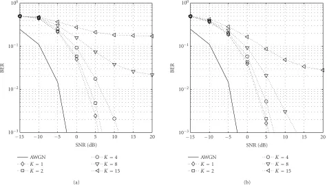
Figure4: Performance of the presented joint synchronization and detection scheme using the NLS algorithm (Nc=15,ψ=0.248,δ=100).
(a)Nite=Nt=127 and (b)Nite=Nt=255.
Figure 2b plots the average MSE as a function of the synchronization error showing how on average the syn-chronization error is minimized by (41). However, the syn-chronization error may be nonzero and the performance of the receiver therefore degrades, as the captured energy be-comes less. This, along with the fact that in the two cases shown only Nite = 127 andNite = 255 iterations are
per-formed, explains why the BER in Figure 4 degrades com-pared to that of Figure 3, especially when more users are added. This performance degradation is the price paid by using this low-complexity type of joint synchronization and detection. However, the achieved performance is the same as could be reached by using the RLS algorithm, but in the ex-ample whereNite=127, the NLS algorithm lowers the
com-plexity by a factor ofG(Nite)10 resulting in approximately
20 times the overall complexity reduction.
7. CONCLUSION
A method for performing joint synchronization, channel estimation, and multiuser detection for single-band DS-CDMA UWB communications has been presented based on the principles in [3,8]. Simulations of the receiver show good results in the UWB multipath channel in [9] using RLS adap-tation, but the complexity of the RLS adaptation is very high. To help alleviate this problem, a novel algorithm termed the WNLS algorithm is derived, potentially lowering the compu-tational complexity while preserving the performance of the RLS algorithm.
ACKNOWLEDGMENTS
The author would like to thank the anonymous reviewers for pointing out that the synchronization scheme was already in existence, as the author was unaware of this fact. Further, the author wishes to thank Thomas Fabricius, Spectronic Den-mark, and Associate Professor Jan Larsen, Technical Univer-sity of Denmark, for their various fruitful discussions. In addition, the author greatly appreciates the careful proof-reading by Pedro Højen-Sørensen, Nokia Denmark, and Ole Nørklit, Nokia Denmark.
REFERENCES
[1] Federal Communications Commission (FCC), “Revision of part 15 of the commission’s rules regarding ultra-wideband transmission systems,” First Report and Order, ET Docket 98-153, FCC 02-48; Adopted: February 2002; Released: April 2002.
[2] A. Muqaibel, A. Safaai-Jazi, B. Woerner, and S. Riad, “UWB channel impulse response characterization using deconvolu-tion techniques,” in Proc. 45th IEEE Midwest Symposium on Circuits and Systems (MWSCAS ’02), vol. 3, pp. 605–608, Tulsa, Okla, USA, August 2002.
[3] U. Madhow, “Adaptive interference suppression for joint ac-quisition and demodulation of direct-sequence CDMA sig-nals,” in Proc. IEEE Military Communications Conference (MILCOM ’95), vol. 3, pp. 1200–1204, San Diego, Calif, USA, November 1995.
[5] R. Smith and S. Miller, “Acquisition performance of an adap-tive receiver for DS-CDMA,” IEEE Trans. Commun., vol. 47, no. 9, pp. 1416–1424, 1999.
[6] M. Latva-aho, J. Lilleberg, J. Iinatti, and M. Juntti, “CDMA downlink code acquisition performance in frequency-selective fading channels,” inProc. 9th IEEE International Symposium on Personal, Indoor and Mobile Radio Commu-nications (PIMRC ’98), vol. 3, pp. 1476–1480, Boston, Mass, USA, September 1998.
[7] M. El-Tarhuni and A. Sheikh, “Performance analysis for an adaptive filter code-tracking technique in direct-sequence spread-spectrum systems,”IEEE Trans. Commun., vol. 46, no. 8, pp. 1058–1064, 1998.
[8] Q. Li and L. A. Rusch, “Multiuser detection for DS-CDMA UWB in the home environment,” IEEE J. Select. Areas Com-mun., vol. 20, no. 9, pp. 1701–1711, 2002.
[9] D. Cassioli, M. Z. Win, and A. F. Molisch, “The ultra-wide bandwidth indoor channel: from statistical model to simula-tions,”IEEE J. Select. Areas Commun., vol. 20, no. 6, pp. 1247– 1257, 2002.
[10] M. Z. Win and R. A. Scholtz, “Impulse radio: how it works,” IEEE Commun. Lett., vol. 2, no. 2, pp. 36–38, 1998.
[11] H. V. Poor and S. Verdu, “Probability of error in MMSE mul-tiuser detection,” IEEE Trans. Inform. Theory, vol. 43, no. 3, pp. 858–871, 1997.
[12] S. Haykin, Adaptive Filter Theory, Prentice-Hall, Upper Sad-dle River, NJ, USA, 3rd edition, 1996.
[13] L. P. B. Christensen, “Signal processing for ultra-wideband systems,” M.S. thesis, Informatics and Mathematical Mod-elling, Technical University of Denmark, Lyngby, Denmark, May 2003,http://www.imm.dtu.dk/∼lc.