Regularized estimation of Euler pole parameters
Bahadır Aktu˘g1and ¨Omer Yıldırım2
1Geodesy Department, Kandilli Observatory and Earthquake Research Institute, Bogazici University, 34684 Cengelkoy, Istanbul, Turkey 2Department of Surveying Engineering, Gaziosmanpas¸a University, 60250 Tokat, Turkey
(Received December 5, 2011; Revised September 29, 2012; Accepted October 20, 2012; Online published August 23, 2013)
Euler vectors provide a unified framework to quantify the relative or absolute motions of tectonic plates through various geodetic and geophysical observations. With the advent of space geodesy, Euler parameters of several relatively small plates have been determined through the velocities derived from the space geodesy observations. However, the available data are usually insufficient in number and quality to estimate both the Euler vector components and the Euler pole parameters reliably. Since Euler vectors are defined globally in an Earth-centered Cartesian frame, estimation with the limited geographic coverage of the local/regional geodetic networks usually results in highly correlated vector components. In the case of estimating the Euler pole parameters directly, the situation is even worse, and the position of the Euler pole is nearly collinear with the magnitude of the rotation rate. In this study, a new method, which consists of an analytical derivation of the covariance matrix of the Euler vector in an ideal network configuration, is introduced and a regularized estimation method specifically tailored for estimating the Euler vector is presented. The results show that the proposed method outperforms the least squares estimation in terms of the mean squared error.
Key words:Tectonics, Euler parameters, multicollinearity, GNSS velocities.
1.
Introduction
The motion of tectonic plates is usually parameterized on a sphere through an Euler vector or an Euler pole (DeMets
et al., 1990; Altamimi et al., 2002; Sella et al., 2002). Such a parameterization is also useful to compare the es-timates from different sources such as space geodetic mea-surements, hot-spots tracks, transform fault azimuths, the spreading rates of ocean ridges, and earthquake slip vec-tors (Gripp and Gordon, 1990, 2002; Argus and Gordon, 1991; DeMets et al., 1994, 2010). However, all the non-geodetic methods give, in fact, only a relative measure of the plate motions. Even the direct geodetic measurements of plate motions depend on the underlying reference frame (Altamimiet al., 2002; Kreemeret al., 2003; Prawirodirdjo and Bock, 2004). Since only the relative motion of the plates can be directly observed, they are often referenced with respect to either a specific plate or a global plate cir-cuit, called no-net-rotation. Thus, the Euler vectors are nec-essary to compute the global plate circuit closure and to quantify the relative motions of tectonic plates.
The Euler parameterization of tectonic plate motions pro-vides an indispensible tool for modeling the rigid plates where the deformation along the plate boundaries are ne-glected or assumed comparatively small (McCluskyet al., 2000; Nocquetet al., 2001; Aktu˘get al., 2009a, b). Even in those models which take the deformation along plate boundaries into consideration, the Euler parameterization is still employed with the compensation of the deformation
Copyright cThe Society of Geomagnetism and Earth, Planetary and Space Sci-ences (SGEPSS); The Seismological Society of Japan; The Volcanological Society of Japan; The Geodetic Society of Japan; The Japanese Society for Planetary Sci-ences; TERRAPUB.
doi:10.5047/eps.2012.10.004
along plate boundaries through elastic back-slip modeling (McCaffrey, 1996, 2002; Meade and Hager, 2005). In this respect, a reliable estimation of the Euler vector is impor-tant in many studies ranging from the estimation of slips along plate boundaries and paleomagnetic studies to the re-construction of the plate tectonics. It is common to esti-mate an Euler vector for a plate motion through the velocity vectors obtained from the geodetic measurements. On the other hand, since quantifying the motion of tectonic plates requires a rigidity assumption, the geometrical coverage of the available velocity vectors is limited to the rigid parts of the plate in question. This results in a weakly multi-collinear estimation problem, especially for smaller plates. Such multicollinearity can be observed in the high correla-tion between the Euler vector components, as well as be-tween the Euler pole and its angular velocity. The corre-lations can be to such an extent that the Euler pole posi-tion and its angular rotaposi-tion rate cannot be estimated di-rectly. This is chiefly due to the matrix singularity of the normal equation matrix, which arises from the collinearity of the rotation rate with either latitude or longitude of the Euler pole. One common solution is to estimate the Euler vector and then transform it to the Euler pole parameters. However, the correlations between the Euler vector compo-nents are still close to unity, which still presents a weakly multicollinear problem. The multicollinearity in the esti-mation of Euler vectors is often coupled with errors which come from the non-rigid behavior of the sites. Up to 3–4 mm/yr residuals are common after removing the Euler ro-tation from the site velocities (Qianget al., 1999; Nocquet
et al., 2001; Aktu˘get al., 2009b). The multicollinearity in the estimation problems is often handled with Tykhonov-Phillips regularization (Tykhonov, 1963; Tykhonov-Phillips, 1962).
While the required Tykhonov matrix is obvious in many ap-plications, due to geometrical or physical relations such as the smoothness of the geophysical signal over a spatial or temporal domain, the components of the Euler vector are discrete and no such simple relations between parameters are available for Euler vector components. For instance, no direct assumption can be made about any smoothness or closeness between Euler vector components.
Another common choice for the Tykhonov matrix is the identity matrix. This approach is useful to stabilize a singu-lar problem numerically and leads to a minimum norm solu-tion, but it has no physical or geometrical meaning for Euler vector components. Consequently, the necessary Tykhonov matrix, which can be used in the regularized estimation of the Euler vector, is not available and has to be developed analytically as implemented in this study.
In this study, the concept of an ideal distribution of the velocity vectors is introduced, the necessary Tykhonov ma-trix was derived analytically, and the multicollinearity be-tween Euler parameters was handled with regularization. The results show that the suggested methodology outper-forms the standard least squares in terms of the Mean Squared Error (MSE) and decreases the correlation among the Euler vector components.
2.
Regularized Estimation of the Euler Vector
Since the derivation of the necessary regularization ma-trix for the Euler vector and the associated equations will be based on the least-squares, the estimation model will be given very briefly for completeness rather than a complete summary. The estimation of the Euler vector from a set of velocities can be formulated in a Gauss-Markov model as:e=Aξξξ+W, e∼N(0, e), (1)
whereeis the error vector of the velocities,Ais the matrix of coefficients,ξξξis the unknown Euler vector (ωx˙ ,ωy˙ ,ωz˙ ), andWis the misclosure vector defined as:
W=Aξξξ0−v, (2)
whereξξξ0is thea priorivalues vector of the parameters (ωx˙ ,
˙
ωy,ωz˙ ), and vis the observation vector which consists of the Cartesian velocity components. The coefficients matrix
Ais a function of the mathematical relation between the observed velocity vector and the Euler vector, and can be expressed in tensor notation as:
vk=ξirjεi j k (3)
whereεi j k is the permutation tensor and r is the position vector in Cartesian frame. After rearranging Eq. (3) in a matrix form according to the model in Eq. (1), three rows of the matrixAcorresponding to the velocity vector at site
ican be obtained as;
vi=
The whole coefficient matrixAis formed by stacking (4) for each site. In a standard least squares estimation, thea
posterioricovariance of the Euler vector components can be obtained as:
ξξξˆ =(ATe−1A)−1, (5)
where the subscriptξξξˆis the vector of the estimated parame-ters. Hereafter, in this paper, the hat symbol is used to refer to estimated quantities. Assuminge = σ2Ifor an ideal network configuration, whereσ2 is the variance factor and
Iis the identity matrix, the inverse cofactor matrix of the pa-rameters in Eq. (5) fornsites can be written in an expanded form as:
A regularized estimation for the model Eq. (1) can be for-mulated by imposing a linear stochastic constraint equation
(ξξξ−ξξξ0)=e, withe ∼ N(0, κ−2I), on the parameters and the estimates can be obtained as:
ˆ
ξξξ =ξξξ0−(ATe−1A+κ
2T)−1AT−1
e W, (7)
Tykhonov matrix to estimate the datum transformation pa-rameters from a set of distorted terrestrial network coordi-nates. For the case of Euler vector components, an analyt-ical derivation based on the intrinsic geometranalyt-ical relations between the components of an Euler vector is needed. The regularization can be applied with respect to the inverse co-factor matrix of an ideal network configuration by choosing the quadratic Tykhonov matrix as (Tarantola, 2005):
T=−1
ˆ
ξ . (8)
Assuming that an ideal regional network contains all the theoretically-possible points within a region bounded by the latitudesϕaandϕb, and longitudesλa andλb, the individ-ual summation terms in Eq. (6) can be expressed as surface integrals over the region. Since the region is defined in ge-ographic coordinates, it is more convenient to apply the in-tegration over the geodetic coordinates instead of Cartesian coordinates. For the purpose of the following derivation, a spherical approximation to the transformation between Cartesian and the geodetic coordinate system is sufficient:
xi =R cosϕicosλi, (9)
yi =R cosϕisinλi, (10)
zi =R sinϕi, (11)
whereRis the approximate Earth’s radius. The individual summation terms in the inverse cofactor matrix in (6) can equivalently be expressed as the product of the number of points and the mean values of the functions, and, thus, can be obtained analytically using the integral mean value theorem. The summation terms in (6) can be written as double integrals over the domainϕ=ϕb−ϕa andλ=
λb −λa. Denoting the mean latitude and mean longitude asϕmandλm, respectively, the individual summation terms for a number of points (n) can be written as:
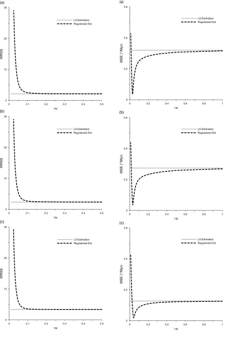
Consequently, the Tykhonov matrix in Eq. (7) can be obtained with respect to an ideal network configuration through Eqs. (12)–(17). The regularization constant is usually obtained through an ad-hoc method (Tarantola, 2005). Various methods such as the L-Curve, generalized cross-validation, maximum likelihood, Morozov’s discrep-ancy principle, quasi-optimality criterion, and the Cp-Plot, have been developed in different contexts (Mallows, 1973; Hansen, 1992; Golub and von Matt, 1997). However, the success of each method to determine the regularization con-stant depends on the specific application (Hoerl and Ken-nard, 1970). One suitable method for one specific problem could have an over-smoothing or under-smoothing effect on another. In general, all the methods employ the variation of the Weighted Residuals Sum of Squares (WRSS) with re-spect to the regularization constant. The chosen constant should balance the WRSS and the constraints. The empiri-cal determination of the regularization constant from WRSS plots is also very common and has been shown to be a suffi-cient method in many geophysical problems (B¨urgmannet al., 2002; Wrightet al., 2003; Aktu˘get al., 2010).
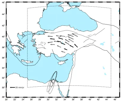
Fig. 1. Three synthetic networks (net #1=black, net #2=white, net #3=gray arrows) and the estimated positions of Euler poles. The ellipses for velocities and the Euler poles are at 95% confidence level. The area with dashed borders represents the borders of an ideal regional network distribution.
distribution is too perfect. Such a non-realistic covariance matrix has also too optimistic error estimates. Using such a covariance matrix corresponds to putting too tight con-straints on thea prioriparameters. However, thea priori
values of the Euler parameters are obtained from many dif-ferent observations of varying accuracy. Therefore, thea priori values are generally less accurate than implied by the covariance matrix of a perfect network distribution. To be able to use less accuratea prioriconstraints while pre-serving the intrinsic correlations of constraints, the cofactor matrix obtained in Eq. (5) can be transformed into a corre-lation matrix and a new inverse cofactor matrix with loose constraints can be formed as:
E=D−1/2ξξξˆD−1/2, (18)
T=
C1x/02E C
1/2 x0
−1
, (19)
whereEis the correlation matrix,Dis the diagonal matrix formed by using the computed covariance asD=diag(ξξξˆ),
Cx0is the diagonal matrix of loosea prioriconstraints fora
priorivalues of the parameters (x0). Cx0 is constructed by
putting the variances of the parameters in the diagonals.
3.
Numerical Application
To demonstrate the efficiency of the regularized estima-tion of Euler vector components, three synthetic velocity fields were formed using a pre-defined Euler vector. The
Table 1. True anda prioriEuler pole parameters.
ϕp λp ω
(◦) (◦) (◦/Myr)
True 32.0000 32.0000 1.4000
A priori 30.0000 31.0000 2.0000
Table 2. Estimated Euler pole parameters with standard least squares.
Net # ϕp λp ω MSE
(◦) (◦) (◦/Myr) (◦/Myr)
1 31.1836 30.8270 1.0812 0.3200
2 30.9492 31.0188 1.1277 0.2739
3 31.6771 31.2491 1.2739 0.1272
typi-Fig. 2. Weighted residual sum of the squares as a function of regularization
Table 3. Estimated Euler pole parameters with regularized method.
Net # ϕp λp ω MSE
(◦) (◦) (◦/Myr) (◦/Myr)
1 31.9541 31.2776 1.2550 0.1457
2 31.7478 31.3165 1.2982 0.1029
3 31.7042 31.3392 1.3141 0.0872
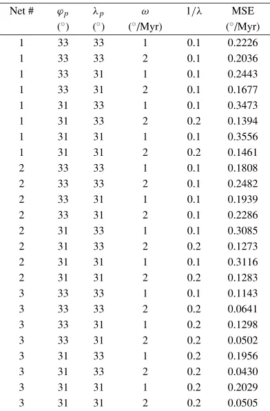
Table 4. MSE values with differenta priorivalues.
Net # ϕp λp ω 1/λ MSE
cal for GNSS observations (Aktu˘get al., 2009b). To suf-ficiently account for the non-rigid behavior of the sites, as well as the possible unmodelled observation errors, a non-rigid deformation of 1–2 mm/yr was also randomly added to the velocities. Such non-rigid behavior is very common in GNNS networks and usually observed in residual veloci-ties with respect to a plate-fixed reference frame (McClusky
et al., 2000; Nocquetet al., 2001). The velocities shown in Fig. 1 include the added noise.
The standard least-squares solutions for the three net-works are given in Table 2. As is clear in Table 2, the Euler vector is highly sensitive to the geometry of the sites. The magnitude of rotation varies up to 0.3◦/Myr, which makes it difficult to compare the results with the results of the stud-ies. In the regularized estimation, the Tykhonov matrix was constructed with loose constraints of 2◦, 2◦and 1◦/Myr for the latitude, longitude and the rotation rate, respectively. Such very loose constraints are compatible with thea pri-orivalues which were deliberately chosen to be imprecise. The regularization constants were determined empirically as 0.10 for all three networks using the WRSS plots of the networks given in Fig. 2, similar to that given in Aktu˘get al.
(2010). The necessary geographical bounds for
construct-ing the Tykhonov matrix were chosen as shown in Fig. 1 by a dashed line. Finally, the Mean Squared errors of both least squares and the proposed method was computed as:
tr(MSE(xˆ))=tr
Ex− ˆx x− ˆxT
, (20)
whereE{·},xandxˆ are the expectation operat¨or, the true values vector, and the estimated values vector of the pa-rameters, respectively. The results of regularized estimation are given in Table 3. The MSE plots of both standard least squares and regularized estimation are given in Fig. 3.
To investigate the effect of differenta priorivalues, the numerical study was repeated with different sets ofa priori
values. The regularization constant was chosen separately for each set. The different sets ofa priorivalues, and the MSE of each trial, are given in Table 4.
4.
Results and Conclusion
The Euler vector has been an indispensible tool for mod-eling plate tectonics, as well as for approximating the rigid motion of sites. However, the number of sites located in the rigid parts of the plates is often limited. Such a limitation is often coupled with uncertainty about the rigid behavior of a site represented in the residuals of the velocities defined in plate-fixed frames. Considering that the estimation model of Euler vectors is in an Earth-centered Cartesian frame, the velocity vectors on a small plate provides a limited ge-ographic coverage, presenting a multicollinear problem.
It has been shown that a very similar network configura-tion can make a huge difference in the estimated parame-ters. For many regional networks, either the latitude or the longitude of the Euler pole is nearly collinear with the mag-nitude of the rotation rate, such that an iterative solution does not converge in the direct estimation of the Euler pole parameters. In the given example, the latitude of the Euler pole is highly correlated with the rotation rate since the Eu-ler pole is almost in the south of the Anatolian plate. The normal equation matrix is a function of the geometry of the distribution of the network, and the condition number of the normal equation matrix is an indication of how well-posed the problem is. Ill-posed problems are generally identified by the high condition numbers of the normal equation ma-trix (Hansen, 2010). For instance in the given examples, while the condition number of the normal equation matrix in a direct estimation of the Euler pole parameters is about
The smaller is the regularization constant, the closer will be the estimate to the standard least-squares. Regardless of the MSE performance, the proposed method also provides a homogenous framework to compare the results of different studies.
Acknowledgments. The authors would like to thank the Editor and two anonymous reviewers for their valuable comments and suggestions to improve the manuscript. All the figures were pre-pared using the software of Wessel and Smith (1995).
References
Aktu˘g, B., Weakly Multicollinear Datum Transformations,J. Surv. Eng., 138(4), 184–192, 2012.
Aktu˘g, B., O. Lenk, M. A. G¨urdal, and A. Kilicoglu, Establishment of re-gional reference frames for detecting active deformation areas in Ana-tolia,Stud. Geophys. Geod.,2, 53, 169–183, 2009a.
Aktu˘g, B., J. M. Nocquet, A. Cingoz, B. Parsons, Y. Erkan, P. England, O. Lenk, M. A. Gurdal, A. Kilicoglu, H. Akdeniz, and A. Tekgul, Deformation of western Turkey from a combination of permanent and campaign GPS data: Limits to block-like behavior,J. Geophys. Res., 114, B10404, 2009b.
Aktu˘g, B., B. Kaypak, and R. N. C¸ elik, Source parameters of 03 February 2002 C¸ ay Earthquake, Mw6.6 and aftershocks from GPS Data, South-western Turkey,J. Seismol.,14, 445–456, 2010.
Altamimi, Z., P. Sillard, and C. Boucher, ITRF2000: A new release of the International Terrestrial Reference Frame for earth science applications,
J. Geophys. Res.,107(B10), 2114, doi:10.1029/2001JB000561, 2002. Argus, D. F. and R. G. Gordon, No-net-rotation model of current plate
velocities incorporating plate motion model NUVEL-1,Geophys. Res. Lett.,18, 2039–2042, 1991.
B¨urgmann, R., M. A. Ayhan, E. J. Fielding, T. Wright, S. McClusky, B. Aktug, C. Demir, O. Lenk, and A. T¨urkezer, Deformation during the 12 November 1999, D¨uzce, Turkey Earthquake, from GPS and InSAR Data,Bull. Seismol. Soc. Am.,92, 161–171, 2002.
DeMets, C., R. G. Gordon, D. F. Argus, and S. Stein, Current plate mo-tions,Geophys. J. Int.,101, 425–478, 1990.
DeMets, C., R. G. Gordon, D. F. Argus, and S. Stein, Effect of recent revisions to the geomagnetic reversal time scale on estimates of current plate motions,Geophys. Res. Lett.,21, 2191–2194, 1994.
DeMets, C., R. G. Gordon, and D. F. Argus, Geologically current plate motions,Geophys. J. Int.,181, 1–80, 2010.
Flores, A., G. Ruffini, and A. Rius, 4D tropospheric tomography using GPS slant wet delays,Ann. Geophys.,18, 223–234, 2000.
Golub, G. and U. von Matt, Tikhonov regularization for large scale prob-lems, Stanford SCCM Report, 97-03, Stanford, California, 1997. Gripp, A. E. and R. G. Gordon, Current plate velocities relative to the
hotspots incorporating the NUVEL-1 global plate motion model, Geo-phys. Res. Lett.,17, 1109–1112, 1990.
Gripp, A. E. and R. G. Gordon, Young tracks of hotspots and current plate velocities,Geophys. J. Int.,150, 321–361, 2002.
Hansen, P. C., Analysis of discrete ill-posed problems by means of the L-curve,SIAM Rev.,34, 561–580, 1992.
Hansen, P. C.,Discrete Inverse Problems: Insight and Algorithms, SIAM, Philadelphia, 2010
Hoerl, A. E. and R. W. Kennard, Ridge regression: Biased estimation for nonorthogonal problems,Technometrics,12, 55–67, 1970.
Howe, B. M., K. Runciman, and J. A. Secan, Tomography of ionosphere: Four dimensional simulations,Radio Sci.,33(1), 109–128, 1998. Kreemer, C., W. E. Holt, and A. J. Haines, An integrated global model of
present-day plate motions and plate boundary deformation,Geophys. J. Int.,154, 8–34, 2003.
Mallows, C. L., Some comments on Cp,Technometrics, 15, 661–675, 1973.
McCaffrey, R., Estimates of modern arc-parallel strain rates in forearcs,
Geology,24, 27–30, 1996.
McCaffrey, R., Crustal block rotations and plate coupling, inPlate Bound-ary Zones, edited by S. Stein and J. Freymueller, AGU Geodynamics Series,30, 101–122, 2002.
McClusky, S., S. Bassalanian, A. Barka, C. Demir, S. Ergintav, I. Georgiev, O. Gurkan, M. Hamburger, K. Hurst, H.-G. Hans-Gert, K. Karstens, G. Kekelidze, R. King, V. Kotzev, O. Lenk, S. Mahmoud, A. Mishin, M. Nadariya, A. Ouzounis, D. Paradissis, Y. Peter, M. Prilepin, R. Relinger, I. Sanli, H. Seeger, A. Tealeb, M. N. Toksaz, and G. Veis, Global Positioning system constraints on plate kinematics and dynamics in the eastern Mediterranean and Caucasus,J. Geophys. Res.,105(B3), 5695–5719, 2000.
Meade, B. J. and B. H. Hager, Block models of crustal motion in southern California constrained by GPS measurements,J. Geophys. Res.,110, B03403, 2005.
Nocquet, J. M., E. Calais, Z. Altamimi, P. Sillard, and C. Boucher, In-traplate deformation in western Europe deduced from an analysis of the International Terrestrial Reference Frame 1997 (ITRF97) velocity field,
J. Geophys. Res.,106(B6), 11239–11257, 2001.
Phillips, D. L., A technique for the numerical solution of certain integral equations of the first kind,J. Assoc. Comput. Mach.,9, 84–96, 1962. Prawirodirdjo, L. and Y. Bock, Instantaneous global plate motion model
from 12 years of continuous GPS observations,J. Geophys. Res.,109, B08405, 2004.
Qiang, Z., Z. Wenyao, and X. Yongqin, Global plate motion models in-corporating the velocity field of ITRF96,Geophys. Res. Lett.,26(18), 2813–2816, 1999.
Sella, G., T. Dixon, and A. Mao, REVEL: A model for recent plate veloc-ities from space geodesy,J. Geophys. Res.,107(B4), 2002.
Tarantola, P.,Inverse Problem Theory, SIAM, Philadelphia, 2005. Tykhonov, A. N., The regularization of incorrectly posed problems,Soviet
Math. Doklady,4, 1624–1627, 1963.
Wessel, P. and W. H. F. Smith, New version of the generic mapping tools released,Eos Trans. AGU,76(329), 1995.
Wright, T. J., Z. Lu, and C. Wicks, Source model for the Mw 6.7, 23 October 2002, Nenana Mountain Earthquake (Alaska) from InSAR,
Geophys. Res. Lett.,30(18), 2003.