R E S E A R C H
Open Access
Cyclic block filtered multitone modulation
Andrea M Tonello
*and Mauro Girotto
Abstract
A filter bank modulation transceiver is presented. The idea is to obtain good sub-channel frequency confinement as it is done by the family of exponentially modulated filter banks that is typically referred to as filtered multitone (FMT) modulation. However, differently from conventional FMT, the linear convolutions are replaced with circular
convolutions. Since transmission occurs in blocks, the scheme is referred to as cyclic block FMT (CB-FMT). This paper focuses on the principles, design, and implementation of CB-FMT. In particular, it is shown that an efficient realization of both the transmitter and the receiver is possible in the frequency domain (FD), and it is based on the concatenation of an inner discrete Fourier transform (DFT) and a bank of outer DFTs. Such an implementation suggests a simple sub-channel FD equalizer. The overall required implementation complexity is lower than in FMT. Furthermore, the orthogonal filter bank design is simplified. The sub-channel frequency confinement in CB-FMT yields compact power spectrum and lower peak-to-average power ratio than in OFDM. Furthermore, the FD equalization allows the exploitation of the transmission medium time and frequency diversity; thus, it potentially yields lower symbol error rate and higher achievable rate in time-variant frequency-selective fading.
Keywords: Filter bank modulation; Multi-carrier modulation; FMT; OFDM; Power spectral density; PAPR; Fading channels; Equalization
1 Introduction
Filter bank modulation (FBM) systems, also referred to as multicarrier modulation systems, have been success-fully applied to a wide variety of digital communication applications over the past several years. The research of improved solutions is still large because of the increasing demand for broadband telecommunication services both over wireline and wireless channels.
Wideband channels are characterized by frequency selectivity which translates in time-dispersive impulse responses that cause significant inter-symbol interference (ISI) in digital communication systems. FBM transceivers employ a transmission technique where a set of narrow band signals (low data rate sequences) are transmitted simultaneously over a broadband channel [1]. In partic-ular, each low rate data sequence is transmitted through a sub-channel that is shaped according to a sub-channel pulse. If the sub-channels are sufficiently narrowband, they will experience an overall flat frequency response so that the medium frequency selectivity does not intro-duce significant inter-carrier interference (ICI) and ISI.
*Correspondence: [email protected]
University of Udine, Wireless and Power Line Communications Lab, Via delle Scienze 208, Udine 33100, Italy
Therefore, the channel equalization task can be simplified. More in general, FBM architectures aim to increase the system spectral efficiency, to enable the agile use of spec-trum and the flexible adaptation of available resources.
Two baseline FBM solutions are orthogonal frequency division multiplexing (OFDM) [2] and filtered multitone (FMT) modulation [3]. FMT consists of an exponentially modulated filter bank that privileges the sub-channel fre-quency confinement rather than the time confinement, as for example OFDM does. In FMT, with frequency confined pulses, the sub-channels are quasi-orthogonal to each other which prevents the system to suffer from ICI, while the ISI introduced by the frequency-selective medium can be mitigated with sub-channel equaliza-tion [3,4] or with the use of outer OFDM modules, one per sub-channel, as described in the concatenated OFDM-FMT scheme in [5]. Clearly, to obtain high sub-channel frequency confinement, long prototype pulses are required. In such a case, the implementation complexity may increase significantly. Therefore, the efficient FMT implementation as well as the design of good pulses is an important aspect [6-10].
In this paper, a novel FBM scheme is described. The ambitious goal is to merge the strengths of both OFDM
and FMT. We refer to it as cyclic block filtered multitone modulation (CB-FMT). Similarly to conventional FMT, CB-FMT aims at generating well frequency localized sub-channels. However, differently from it, CB-FMT transmits data symbols in blocks, and the filter bank does not use linear convolutions but cyclic convolutions. Similarly to OFDM, the block transmission can reduce latency, but the sub-channel frequency confinement is much higher, more similarly to FMT. This translates in higher spec-tral selectivity, more confined power specspec-tral density, and lower peak-to-average-power ratio (PAPR) than in OFDM given the same target spectral efficiency. Further-more, the implementation complexity is lower than that in FMT with the same number of sub-channels and even with longer pulses. In fact, an efficient realization can be devised if both the synthesis and the analysis filter banks in CB-FMT are implemented in the frequency domain (FD) via a concatenation of an inner (with respect to (w.r.t.) the channel) discrete fourier transform (DFT) and a bank of outer DFTs. Such a FD architecture enables the use of a FD sub-channel equalizer designed according to the zero forcing (ZF) or the minimum mean square error (MMSE) criterion [11]. In particular, the ZF solution will restore perfect orthogonality if a cyclic prefix (similarly to OFDM) is appended to each block of signal coefficients that are transmitted over a dispersive (frequency selec-tive) channel. In the presence of channel time variations (because of mobility), the ICI is small due to the sub-channel frequency confinement so that the sub-sub-channel equalizer is sufficient to cope with the ISI experienced by the data symbols transmitted in a block. This equalization scheme is capable to coherently collect the sub-channel energies so that frequency and time diversity, offered by the fading channel, can be exploited. Consequently, this can provide better performance, i.e., lower symbol error rate and higher achievable rate, than OFDM.
The CB-FMT idea and principles were originally pre-sented in [12]. Some aspects related to the FD implemen-tation were disclosed more recently in [13], while in [14] a preliminary analysis of the robustness of the scheme in fading channels was reported. In this paper, we provide a detailed description of CB-FMT with emphasis to the design, implementation, equalization, and performance aspects.
Another FBM scheme referred to as generalized OFDM (GFDM) has been independently presented in [15]. According to [15], GFDM is a FBM scheme that uses a non-orthogonal design where the sub-channel spacing is smaller than the sub-channel Nyquist band. It can be viewed as an FMT scheme operating beyond the critical sample rate. An extended CP is used to take into account the pulse tails and allow the implementation of a so-called tail biting convolution. The tail biting convolution in turn can be implemented with a circular convolution. Since
the design is not orthogonal, ICI is present also in an ideal channel which requires some form of equalization to mitigate it. This may yield performance that is worse than OFDM. However, it is shown in [15] that other benefits are offered by GFDM as spectrum agility and lower PAPR. CB-FMT is a more general architecture than GFDM that shares the idea of using circular convolu-tions instead of linear convoluconvolu-tions. As FMT essentially represents a general exponentially modulated filter bank with linear convolutions, CB-FMT represents a general exponentially modulated filter bank with circular convo-lutions. An orthogonal CB-FMT system can be designed (as done in this paper) without requiring the use of a CP unless more robustness is desirable in time dispersive channels. Orthogonal CB-FMT can offer lower BER and higher spectral efficiency compared to OFDM.
The specific contributions of this paper can be summa-rized as follows:
• The CB-FMT key elements are described in
Section 2. These include the derivation of an efficient frequency domain implementation starting from the time domain signal representation (Section 2.1). • The relations between CB-FMT and conventional
FMT/OFDM are briefly described in Section 2.2 to better understand the differences.
• The complexity analysis is carried out in Section 2.3. • The conditions under which the CB-FMT scheme is orthogonal are studied in Section 3. Herein, a simple orthogonal pulse design is also proposed.
• The analytic derivation of the CB-FMT power spectral density (PSD) and the PAPR are discussed in Section 4.
• Equalization in time-variant frequency-selective fading is discussed in Section 5. A sub-channel FD MMSE equalizer is herein proposed.
• Several numerical examples, which include pulse shapes, complexity, PSD and PAPR, as well as symbol error rate (SER) and achievable data rate
comparisons with OFDM, are collected in Section 6.
Finally, the conclusions follow.
2 Cyclic block FMT modulation
Cyclic block filtered multitone modulation is a multi-carrier modulation scheme. As such, a high data rate information sequence is split into a series of K low data rate sequences. We denote thek-th data sequence with a(k)(N), ∈ Z, which corresponds to a stream
of complex data symbols belonging to a certain constel-lation, e.g., M-QAM or M-PSK, transmitted with sym-bol period NT, where T is the sampling period in the system. A normalized sampling period is assumed, i.e.,
sub-channels obtained by partitioning the wideband transmission medium inKsub-bands.
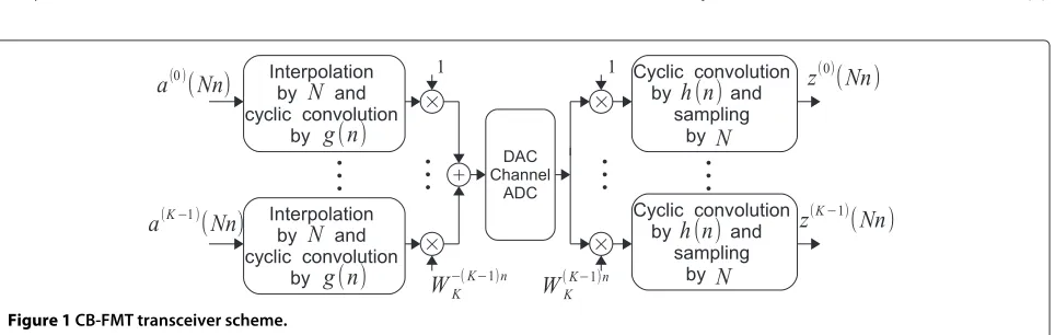
The principle of CB-FMT is depicted in Figure 1. In this scheme, the low data rate data sequences are interpolated by a factorN and, then, filtered with a prototype pulse that is identical for all sub-channels. Differently from con-ventional FMT, the convolutions in the filter bank are circular. The filter outputs are multiplied by a complex exponential to obtain a spectrum translation. Finally, the
K modulated signals are summed together yielding the transmitted discrete time signal.
The circular convolution involves periodic signals, and it can be efficiently realized in the frequency domain via the discrete Fourier transform (DFT). To use the circu-lar convolution, a blockwise transmission is needed. Thus, we gather the low data rate sequences in blocks ofL sym-bolsa(k)(N), ∈ {0,. . .,L−1}, for each sub-channel. Then, we consider the prototype pulseg(n)to be a causal finite impulse response (FIR) filter, with a number of coef-ficients equal toM=LN. If the length is lower thanM, we can extend the pulse length toMwith zero-padding, with-out loss of generality. The CB-FMT transmitted signal can be written as
x(n)= K−1
k=0
a(k)⊗g
(n)
= K−1
k=0 L−1
=0
a(k)(N)g((n−N)M)WK−nk, (1)
n∈ {0,. . .,M−1},
where ⊗denotes the circular convolution operator and
g((n)M)denotes the cyclic (periodic) repetition of the pro-totype pulseg(n)with a period equal toM, i.e.,g((n)M)=
g(mod(n,M))where mod(·,·)is the integer modulo oper-ator.WK−nk = ej2πnk/K is the complex exponential func-tion andjis the imaginary unit.
The signal x(n) is digital-to-analog converted and, then, transmitted over the transmission medium. At the
receiver, after analog-to-digital conversion, the discrete time received signal, denoted withy(), is defined as
y()= P−1
s=0
hCH(s,)x(−s)+η(), ∈Z, (2)
where hCH(s,) is the time-variant channel impulse response andη()is the background noise. In the follow-ing, we assume the channel response to be ideal. The more general case will be discussed in Section 5.
Similarly to the synthesis stage, we can apply the cir-cular convolution to the analysis filter bank. The k-th sub-channel output is obtained as follows:
z(k)(nN)= M−1
=0
y()WKkh((nN−)M), (3)
k∈ {0,. . .,K−1}, n∈ {0,. . .,L−1},
whereh((n)M)denotes the periodic repetition of the pro-totype analysis pulseh(n)with periodM.
Each sub-channel conveys a block of L data symbols over a time period equal toLNT. Therefore, the transmis-sion rate equalsR=K/(NT)symbols/s. More in general, a cyclic prefix can be added (but it is not mandatory) to the transmitted signal, as explained in Section 5. In this case, the rate equals
R= KL
(M+μ)T symbols/s, (4)
whereμis the cyclic prefix length in samples.
2.1 Frequency domain implementation
One of the goals in CB-FMT is the reduction of the computational complexity in the filtering operation w.r.t. the conventional FMT scheme. This can be achieved by exploiting a frequency domain implementation of the system as described in the following.
Firstly, we define a constant integerQsubject to
M=LN=KQ. (5)
Then, theM-point DFT of the transmitted signal in (1) is computed. We obtain
X(i)=
Under the assumptionM=KQ, we can write
X(i)=
SinceM= LN, it should be noted that the summation with indexin (8) is theL-point DFT of the data block
Finally, substituting (9) in (8), we obtain
X(i)= K−1
k=0
A(k)(i−kQ)G(i−kQ), i∈ {0,. . .,M−1}.
(10)
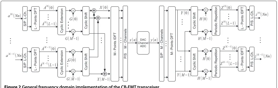
This suggests an implementation of the CB-FMT syn-thesis filter bank as shown in Figure 2. For each sub-channel block of data, we apply anL-point DFT (referred to as outer DFT). We extend cyclically the block of coef-ficients at the output of the outer DFT fromLpoints to
Mpoints. Then, each sub-channel block ofMcoefficients is weighted with the M coefficients G(i) of the proto-type pulse DFT. Next, each sub-channel block is cyclically shifted by a factor−kQ, wherekis the sub-channel index. Finally, the shifted blocks are summed together, and anM -point IDFT (referred to as inner IDFT) is applied to obtain the signal to be transmitted.
If we assume theM-point DFT of the prototype pulse to be confined inQpoints, i.e.,G(i)=0 fori∈ {0,. . .,Q−1}
This suggests an efficient implementation of the CB-FMT synthesis filter bank as shown in Figure 3. For each sub-channel block of data, we apply an L-point DFT (referred to as outer DFT). We extend cyclically the block of coefficients at the output of the outer DFT from L
points to Qpoints. Then, each sub-channel block of Q
coefficients is weighted with theQnon-zero coefficients
G(i)of the prototype pulse DFT. Finally, we apply anM -point IDFT (referred to as inner IDFT) to obtain the signal to be transmitted.
The analysis filter bank can also be implemented in the frequency domain. We start from (3) and we substitute the signaly()with the IDFT of its frequency response as follows:
where in (14) we can recognize the shifted version of the
Figure 2General frequency domain implementation of the CB-FMT transceiver.
where the second equality holds since the signals are peri-odic of M. Considering that M = LN, we have that
WM−(i−kQ)nN =WL−(i−kQ)n, and we can write
z(k)(nN)= M−1
i=0
Y(i)H(i−kQ)WL−(i−kQ)n
= M−1
i=0
Y(i+kQ)H(i)WL−in, (16)
i∈ {0,. . .,M−1},
k∈ {0,. . .,K−1}.
The indexican be decomposed into two indexespandq
asi=p+Lq, withp∈ {0,. . .,L−1}andq∈ {0,. . .,N−1}, to obtain
z(k)(nN)= L−1
p=0 N−1
q=0
Y(p+qL+kQ)H(p+qL)WL−pn.
(17)
In (17), we can recognize theL-point IDFT of the signal
Z(k)(p)that is given by
Z(k)(p)= N−1
q=0
Y(p+qL+kQ)H(p+qL), (18)
p∈ {0,. . .,L−1},
k∈ {0,. . .,K−1}.
This is the periodic repetition with period L of the signal Y(i)H(i − kQ). Therefore, the receiver can be summarized as follows (Figure 2): Firstly, the received signal y(n) is processed with an M-point DFT. Then, the output coefficients are weighted with the proto-type pulse M-point DFT coefficients H(i). Next, a periodic repetition with period L is performed for each sub-channel block of coefficients to obtain (18), where Y(p) is the M-point DFT of the received signal.
Finally, to obtain the k-th sub-channel output, an L -point IDFT is applied to (18), i.e.,
z(k)(nN)= L−1
p=0
Z(k)(p)WL−pn, (19)
n∈ {0,. . .,L−1}, k∈ {0,. . .,K−1}.
Assuming that the analysis pulse has only Qnon-zero coefficients, i.e., H(i) = 0 for i ∈ {Q,. . .,M− 1}, as when the pulse is matched to the synthesis pulse and equal toG∗(i), the pulse weighting and the periodic repetition take place on each sub-channel as graphically depicted in Figure 3. In particular, assumingQ>L, (18) corresponds to adding at the beginning of the block of coefficients
Y(i+kQ)H(i),i∈ {0,. . .,Q−1}the lastQ−Lcoefficients of the same block.
With the orthogonal design that we describe in Section 3, i.e., when H(i) = G∗(i) and assuming that orthogonality conditions are satisfied, we obtain
z(k)(nN)= Q−1
q=0
|G(q)|2a(k)(nN)+N(k)(nN), (20)
which shows that the output sample is equal to then-th data symbol of thek-th sub-channel weighted by the pulse energy, plus a noise contribution. More in general, when the transmission medium is not ideal, equalization can be performed (see Section 5) so that in (20) the coefficient that weights the data symbol is given by the sub-channel energy.
Also the FMT system can be implemented in the fre-quency domain. However, the presence of linear convolu-tions renders it more complex since an overlap-and-add operation has to be carried out as shown in [16].
As a final remark, the use of inner and outer DFTs appeared also in the concatenated OFDM-FMT architec-ture presented in [5].
2.2 Relation with FMT and OFDM
In the following, we briefly highlight the main differences of CB-FMT w.r.t. FMT [3] and OFDM [2]:
2.2.1 Relation with FMT
Similarly to conventional FMT, CB-FMT targets the use of frequency confined sub-channels. However, while the filter banks in FMT deploy linear convolutions, in CB-FMT, the filter banks use cyclic convolutions. Therefore, the FMT transmitted signal does not read as in (1) but as follows:
x(n)= K−1
k=0
∈Z
a(k)(N)g(n−N)WK−nk, n∈Z,
(21)
whereg(n)is the prototype pulse. Furthermore, while in FMT the transmission is typically continuous, in CB-FMT, data signals are transmitted in blocks, each of theK sub-channels transmits a block ofLdata symbols.
In FMT, the rate equals
R= K
NT symbols/s. (22)
The efficient implementation of FMT can exploit a polyphase DFT filter bank architecture [10]. Nevertheless, the FMT complexity is higher than the CB-FMT complex-ity, as shown in Section 2.3 assuming the same number of sub-channels and the same prototype pulse length.
In CB-FMT, very simple frequency domain design can be followed to obtain an orthogonal solution as shown in Section 3. In FMT, the orthogonal design is more con-voluted [9,10]. Thus, non-orthogonal solutions are often adopted in FMT as for instance the use of a truncated root-raised-cosine prototype pulse [3] orad hocfrequency localized pulses [7,8].
When transmission is in time/frequency-selective fad-ing channels, the good sub-channel frequency confine-ment in FMT provides robustness to ICI, while the residual ISI can be mitigated with sub-channel linear equalization [3] or maximuma posteriorisequence estimation [4,17]. In CB-FMT, instead, simple frequency domain equaliza-tion can be adopted as described in Secequaliza-tion 5.
2.2.2 Relation with OFDM
In OFDM, the filter bank privileges the sub-channel time domain localization, rather than the frequency domain localization. OFDM can be seen as a particular case of both FMT and CB-FMT. In fact it corresponds to an FMT system withN =Kand the prototype pulse being a rect-angular window, i.e.,g(n)is equal to 1 forn∈ {0,. . .,N−
1}and 0 otherwise. It follows that the transmitted signal can be expressed as
x(n)= K−1
k=0
a(k)(N)WK−nk, n∈ {N,. . .,(+1)N−1}.
(23)
Starting from CB-FMT, we obtain OFDM by setting
N = K,L = Q= 1, andG(0) = 1, so that we also have
K=M.
In OFDM, the rate equals
R= K
(K+μ)T symbols/s, (24)
2.3 Computational complexity
In this section, we evaluate the computational complex-ity of CB-FMT in terms of number of complex operations [cop] (additions and multiplications) per sample.
Let us assume that anM-point DFT (or IDFT) block has complexity equal toαMlog2(M)[cop] where, for instance,
α=1.2.
At the transmitter,K outer DFTs ofL-points are used, together with oneM-point inner IDFT. Furthermore, the inner IDFT input signals are weighted by the DFT compo-nents of the prototype pulse. Similarly, this applies at the receiver. The operations performed by the cyclic exten-sion is negligible. Let us assume the number of non-zero DFT coeffients of the prototype pulse to be equal toQ2= QC, C ∈ {1,. . .,K}. Since the transmitted block com-prisesLNcoefficients, the number of complex operations per sample is equal to
CCB-FMT= the periodic repetition increases the complexity byS =
2MC−KLfor(Q−L)C < L and byS = (M+KL)C
otherwise. When the prototype pulse has onlyQnon-zero coefficients, i.e.,C = 1,S = Mfor the transmitter and
S=2M−KLfor the receiver.
As a comparison, we consider the complexity of FMT efficiently implemented with a polyphase DFT filter bank as described in [10]. This is equal to
CFMT=
assumingKsub-channels, an interpolation factorN, and a prototype pulse with lengthLg coefficients. This com-plexity does not take into account the operations required by the equalization stage.
If, for example, we assumeK = 64 andN = 80 for both systems and furthermore FMT with a pulse length equal to 20Nwhile CB-FMT withL=K,Q=Nresulting in a longer filter length equal toM = 64N coefficients, the receiver complexity will be equal to{45.8, 21.7} [cop] respectively for FMT and CB-FMT. This shows the gain in complexity of CB-FMT yet having a longer pulse. More results about the complexity are reported in Section 6.2.
3 Orthogonality conditions and prototype pulse design
The frequency domain implementation of CB-FMT allows us to deduce the system orthogonality conditions. A filter bank system is orthogonal when it has the perfect reconstruction property and the transmit-receive filters
are matched, i.e.,g(n)=h∗(−n)andH(i)=G∗(i), so that the system exhibits neither ISI nor ICI [18].
When the prototype pulse satisfies the following two conditions, the CB-FMT system will be orthogonal [19]:
1. TheM -point DFT of the prototype pulse has only Q non-zero coefficients, i.e.,G(i)=0for
i∈ {Q,. . .,M−1}(sufficient condition).
2. The correlation betweeng(n)andg∗(−n), computed with the circular convolution and sampled by a factor N, is the Kronecker delta, i.e.,
3.1 Proof of the orthogonality conditions
To prove the orthogonality conditions, we proceed in two steps. Firstly, we prove the condition to have orthogonal-ity between different sub-channels, i.e., no ICI. Then, we prove the condition to have orthogonality between the data symbols of each sub-channel, i.e., no ISI.
3.1.1 Sub-channel orthogonality
The sub-channels will be orthogonal if theM-point DFT of the prototype pulse, G(i), is equal to zero for i ∈ {Q,. . .,M−1}. In this case, there is no ICI.
Proof.We substitute (10) in (18) assumingY(i)= X(i). The input-output relation between theL-point DFT of the data block is given by
Z(k)(p)=
channels, the terms in the second summation must be zero fork = k. This is possible whenG(q)(p−kkQ)
is equal to zero for kk = 0 and ∀p ∈ {0,. . .,L−
1},∀q ∈ {0,. . .,N−1}. This condition is satisfied when
G(p+qL−kkQ)=0, only forp+qL∈[ 0,. . .,Q−1].
3.1.2 Block orthogonality
Proof. Under the sub-channels orthogonality (previous condition) and with matched filters, (28) becomes
Z(k)(p)=A(k)(p) N−1
q=0
G(q)(p) G(q)(p)∗. (29)
To have perfect reconstruction, we need to have [19]
N−1
q=0
G(p+Lq)G∗(p+Lq)=1, ∀p∈ {0,. . .,L−1}.
(30)
In (30), the summation represents a periodic repetition ofG(p+qL)G∗(p+qL). In the time domain, this translates in sampling by a factorM/L = N. Thus, if we apply an
L-point IDFT to (30), we will obtain (27).
3.2 Orthogonal prototype pulse design
The frequency domain implementation and the orthog-onality conditions suggest to synthesize the pulse in the frequency domain with a finite number of frequency components.
We start by choosing a pulse that belongs to the Nyquist class with roll-off β, Nyquist frequency 1/(2NT), total bandwidth 1/(KT), and frequency responseGˆ(f). Then, we set M. The coefficients in the frequency domain of the CB-FMT prototype pulse are obtained by sampling
the response onlyQout ofMcoefficients are non-zero, whileL < Q
coefficients fall in the the band 1/(NT). It should also be noted that there is a limiting condition on the choice of the roll-offβ. In fact, the maximum roll-off to prevent the pulse tails from exceeding the bandwidth 1/(KT) of Q -points isβmax = (Q−L)/Q. Therefore, we must choose
β ≤βmax.
We recall that the parameters of CB-FMT are related to each other through the relationM = LN = KQ, which can be rearranged as
N
wherepandqare relative prime integers. Therefore, once we have chosenM, the number of sub-channelsK, and the ratioN/K, we obtain the rest of the parametersN,Q,L.
Some examples of pulse responses are reported in Section 6.1. An optimal pulse design method that targets the maximization of the in-band-to-out-of-band pulse energy has been recently presented in [19]. In particu-lar, complex asymetric pulses are also considered. It is also interesting to note that a trivial orthogonal solution is obtained by using a rectangular FD window ofQ non-zero coefficients [20]. In such a case, the CB-FMT scheme
becomes the dual of the OFDM system that uses, instead, a rectangular window in the time domain.
4 PSD- and PAPR-related aspects 4.1 PSD-related aspects
In this section, we study the power spectral density (PSD) of the transmitted CB-FMT signal. The PSD is an impor-tant aspect to evaluate the confinement of the transmitted spectrum. The objective is to limit the out-of-band emis-sions. More in general, the PSD must comply to regulatory aspects that typically set an upper limit, also known as spectrum mask, e.g., as in the IEEE 802.11 WLAN stan-dard [21] or in the HomePlug PLC system [22].
To derive an analytic expression for the PSD of CB-FMT, we can start by expressing the (continuous) transmission of samplesx(n)as follows:
where the sub-channel symbol period M1 = M + μ
takes into account the fact that a cyclic prefix (CP) of lengthμsamples can be used for the equalization, as it will be explained in Section 5. The CP is appended to the block of coefficients at the inner IDFT output. Fur-thermore,X(k)(mM1) are the coefficients at the input of the inner IDFT in the transmitter at time instant mM1,
and gP(n) is the rectangular window that is equal to 1 forn ∈ {0,. . .,M1−1}and zero otherwise. Essentially, X(k)(mM1)represents the block of coefficients defined in
(11) that is transmitted in them-th CB-FMT block. The data symbols a(k)(N) are assumed to be independent, identically distributed with zero mean and power equal to
Ma=E[|a(k)(N)|2].
To convert the signal in (32) from discrete time to con-tinuous time, an interpolation filter with responsegI(t)is
needed. The interpolated signal can be expressed as
x(t)= n∈Z
x(n)gI(t−nT), t∈R. (33)
To obtain the signal PSD, the correlation ofx(t), namely
rx(t,τ)= E[x∗(t+τ)x(t)] whereE[·] is the expectation
operator, needs to be computed. Since the interpolated signal is cyclo-stationary, the correlation is periodic [23], i.e.,rx(t+T,τ)=rx(t,τ). To remove the dependency on the variablet, the mean correlationrx(τ)= T1
T
0 rx(t,τ)dt
The correlation can be written as crete time transmitted signal before the analog interpola-tion filter. To compute (34), we rewrite (32) as
x(n)=
represents the correlation between the sig-nal coefficients at the input of the inner IDFT of the transmitter. We obtain
Consequently, the mean PSD is
Px(f)=
1
TR(f)|GI( f)|
2, (39)
whereR( f)is the discrete Fourier transform of (38).
Assuming that the prototype pulse DFT has onlyQ non-zero coefficients, (37) can be rewritten as
E X(a1+b1Q)(1M1)∗X(a2+b2Q)(2M1)
Then, the PSD can be written as
Px( f)= |GI( f)|2
in the two sums and thus in two resulting terms:
Px(f)=P1( f)+P2( f). (43)
whereGI(f)is the Fourier transform of the analog inter-polation filter. The first term, P1( f), is a sum of sinc functions, each centered infk,qand weighted by the
pro-totype pulse DFT coefficients. The main lobe of the sinc function has a bandwidth equal to 1/ ((M+μ)T). The second term,P2( f), is related to the correlation between the signal coefficientsX(i)at the input of the inner IDFT, defined in (11). In detail, we may reconsider (11). In fact, such coefficients can be written as
X(i)=A(k)(i−kQ)G(i−kQ), (46)
X(i+L)=A(k)(i+L−kQ)G(i+L−kQ)
=A(k)(i−kQ)G(i+L−kQ), (47)
The correlation between (46) and (47) will not be null ifQ > L. This is due to the fact that the block of coeffi-cientsA(k)(i), at the output of the outer DFT, is cyclically
extended. Equation 45 takes this correlation into account.
4.2 PAPR-related aspects
The peak-to-average power ratio (PAPR) is a measure of the transmitted signalx(t), defined as
PAPR= maxt∈R
|x(t)|2
E|x(t)|2 . (48)
The PAPR indicates how much the signal peak power is higher than the mean power value. A signal with high PAPR exhibits high dynamic range. Consequently, this poses a challenge to the analog components of the front end which may introduce distortions. For exam-ple, if the signal exceeds the power amplifier dynamic range, the output signal will be clipped to the supply voltage level. In turn, unintentional out-band interfer-ence due to spurious emissions is generated as well as the signal distortion may cause a performance loss in the receiver stage. In OFDM, the high PAPR is a known drawback. It grows exponentially with the sub-channel number [24]. Generally, the PAPR cannot be expressed in closed-form.
In OFDM, |x(t)| can be approximately modeled as a Rayleigh process as shown in [25] so that pseudo-closed expressions for the distribution of the PAPR can be derived. In CB-FMT, the problem is more complex, so that we have to resort to a numerical approach to evaluate the PAPR as it will be discussed in Section 6.3.
5 Equalization in time-variant frequency-selective channels
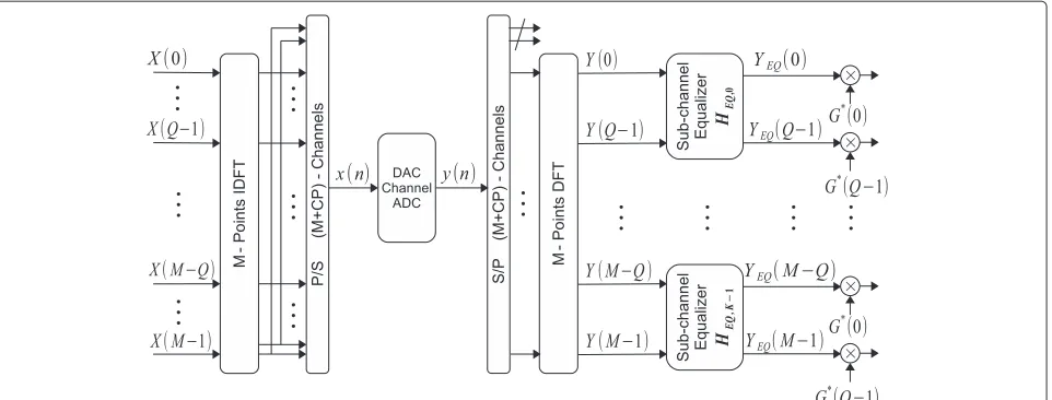
The orthogonality conditions, described in Section 3, ren-der CB-FMT free from interference when the channel is static and has a flat frequency response. When the channel is frequency selective and/or time variant, some inter-ference may be present. However, orthogonality can be restored with an equalizer. From the frequency domain implementation of CB-FMT (Figure 3), we note that the chain comprising theM-point inner IDFT at the trans-mitter, the transmission medium, and theM-point inner DFT at the receiver is similar to the OFDM system. This suggests to append a CP ofμsamples to the transmitted block of samples, as shown in Figure 4.
To proceed, let us denote the time-variant channel response as follows
whereP < μis the channel impulse response length in samples, andαs(n)is thes-th channel tap at time instant n. Then, the received signal can be written as
y(n)= P−1
s=0
hCH(s,n)x(n−s). (50)
To simplify the notation, we focus on the first received block, without loss of generality. After CP removal, under the assumption that the channel duration (in samples) is shorter than the CP, (50) becomes a circular convolution between the transmitted signal and the channel impulse response. In matrix form, we can write
y=HCHx (51)
where y =[y(μ) y(μ+1) . . . y(M+μ− 1)]T, x =
[x(0)x(1) . . . x(M−1)]TandH
CHis the circulant
chan-nel matrix of sizeM×M. The i-th element of the j-th channel matrix column is defined as
{HCH}ij= receiver does through the inner DFT, we will obtain
Y=FMHCHx=FMHCHFHMX= ˆHCHX, (53)
whereFMis theM-point DFT matrix, defined as{FM}ij= WMij/√M,i,j ∈ {0,. . .,M− 1}, andX is the vector of coefficients at the input of the inner IDFT at the transmit-ter side. Essentially, (53) describes the relation that exists between the coefficients at the input of the inner IDFT at the transmitter side and the coefficients at the output of the inner DFT at the receiver side. Such a relation suggests the use of a frequency domain equalizer applied at the out-put of the receiver inner DFT as shown in Figure 4. To proceed, we need to derive an expression for the elements of the matrixHˆCH.
Figure 4Cyclic prefix and frequency domain equalization in CB-FMT.
whereH1(p,n)is theM-point DFT of the channel impulse response at time instantn, i.e., computed along the vari-able. By computing theM-point DFT of (54), we obtain the elements of the vector (53):
Y(q)= M−1
n=0 M−1
p=0
X(p)H1(p,n)WM−pnWMqn
= M−1
p=0
X(p)H2(p,q−p), (55)
q∈ {0,. . .,M−1},
where H2(p,q) is the two-dimensionalM-point DFT of
hCH(,n), defined as
H2(p,q)= M−1
s=0 M−1
n=0
hCH(s,n)WMsp+nq. (56)
Finally, it follows that the elements ofHˆCHare defined as
ˆ
HCH
ij=H2
j, mod(i−j,M). (57)
To derive the FD equalizer, we distinguish between the case of having a time-invariant channel and the case of having a time-variant channel.
5.1 Time-invariant channel
When the channel is time-invariant,hCH(,n) does not depend on the time instantn. Thus,H2(p,q) is not null only forq=0. Consequently, the channel matrixHˆCHis a
diagonal matrix. TheM-point DFT output, at the receiver stage, can be simply written as follows:
Y(p+kQ)=X(p+kQ)H2(p+kQ, 0)+N(p+kQ), (58)
p∈ {0,. . .,Q−1}, k∈ {0,. . .,K−1},
where N(i), i ∈ {0,. . .,M−1}, are the M-point DFT coefficients of the background noise samples. This shows that there is absence of ICI, i.e., interference among the sub-channels. Therefore, the application of a sim-ple 1-tap frequency domain equalizer is enabled [11]. In particular, with zero forcing, the equalizer output is given by
YEQ(p+kQ)=Y(p+kQ)HEQ,ZF(p+kQ), (59)
HEQ,ZF(p+kQ)= 1 H2(p+kQ, 0),
whereHEQ,ZF(i)is thei-th coefficient of the FD zero forc-ing equalizer. In Figure 4, the matrix HEQ,k, associated
to the k-th sub-channel equalizer, is diagonal. Its p-th diagonal element is equal toHEQ,ZF(p+kQ). In such a case, perfect orthogonality is achieved in the system. That is, after zero forcing equalization, the sub-channel signal is multiplied with the conjugate of the pulse frequency response G∗(p), and it is finally processed by the other stages depicted in Figure 3. Then, the output reads as in (20).
Alternatively, the equalizer coefficients can be designed according to the MMSE principle and they read
HEQ,MMSE(p+kQ)= H
∗
2(p+kQ)
|H2(p+kQ, 0)|2+σ2/|G(p)|2,
(60)
5.2 Time-variant channel
When the channel is time variant, the channel matrix
ˆ
HCH has non-zero elements outside the main
diago-nal. The number of non-zero elements off the diagonal grows with the channel Doppler spread. Theq-th inner DFT output coefficient at the receiver can be written as
Relation (61) shows that a simple 1-tap equalizer cannot fully remove the interference introduced by the time-variant channel and represented by the second additive term in (61). Thus, we propose to use a sub-channel block equalizer that mitigates the interference between the L
symbols transmitted in each of the K-th sub-channels considering the fact the the ICI between distinct sub-channels is small due to their good frequency response confinement.
We start by splitting the matrixHˆCHin blocks ofQ×Q
elements, so that (53) can be written as
⎡ Qcoefficients associated to thek-th sub-channel andNis the background noise vector.Bi,jis aQ×Qmatrix defined
as
Thek-th sub-vector in (62) can be written in order to sep-arate the term of interest from the interference as follows
Yk =Bk,kXk+ K−1
i=0 i=k
Bk,iXi+Nk. (64)
Now, thek-th sub-channel block equalizer output vec-tor is given by
YEQ,k=HEQ,kYk, (65)
where the sub-channel equalizer matrix is computed according to the MMSE criterion. Such a matrix is obtained as
is theQ×Qcorrelation matrix between the vectorXkand
the vectorYk, andRYkYk = E
YkYHk
is theQ×Q auto-correlation matrix of the vector Yk. It should be noted
that the signals Xi, i = k, are treated as noise by the k-th sub-channel block equalizer since the interference that they generate is small due to the sub-channel spectral confinement.
After the sub-channel equalization, the output cients are weighted with the prototype pulse FD coeffi-cientsG∗(i)and, finally, processed by the others stages, as shown in Figures 3 and 4.
6 Numerical results 6.1 Pulse design examples
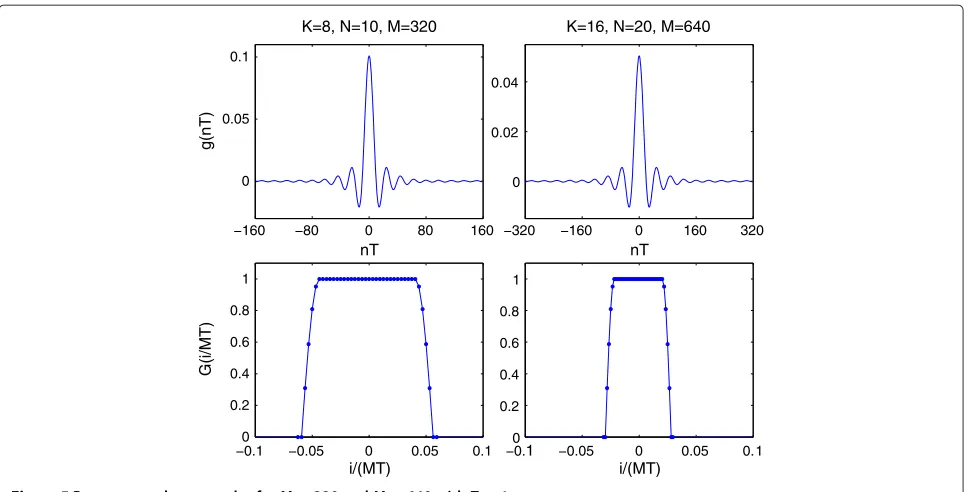
In Figure 5, we report two examples of pulses obtained with the method described in Section 3.2. Several com-binations of parameters are considered. The pulses have been obtained starting from a root-raised-cosine spec-trum with roll-off equal to 0.2. The pulses are designed for
M=320 andM=640. Furthermore,K =8 andN=10 orK=16 andN=20 are considered, respectively.
In Table 1, we report the ratio between the in-band and the out-of-band energy of the interpolated prototype pulse for several choices of the parameters. Despite the simple design method, the pulses exhibit good frequency confinement which increases for larger values ofM.
In all numerical results that will follow, a common con-figuration is related to the case M = 320 and K ∈ {8, 16, 32, 64}.
6.2 Complexity comparisons
In Figure 6, we show the complexity of OFDM, FMT, and CB-FMT as a function of the prototype pulse length (in samples) and assuming it has Q non-zero DFT coeffi-cients. In all FMT, OFDM, and CB-FMT, the pulse length
Lg is set equal toM. It should be noted that OFDM uses
−160 −80 0 80 160 0
0.05 0.1
K=8, N=10, M=320
nT
g(nT)
−320 −160 0 160 320
0 0.02 0.04
K=16, N=20, M=640
nT
−0.1 −0.05 0 0.05 0.1
0 0.2 0.4 0.6 0.8 1
i/(MT)
G(i/MT)
−0.01 −0.05 0 0.05 0.1 0.2
0.4 0.6 0.8 1
i/(MT)
Figure 5Prototype pulse examples forM=320 andM=640 withT=1.
The figure shows that CB-FMT has significant lower complexity than conventional FMT. Clearly, OFDM is the simplest solution. However, CB-FMT and OFDM have a more comparable complexity, i.e., CB-FMT is more complex than OFDM by a factor of about 1.5. As it will be shown in the next sections, this extra complexity pays back since CB-FMT can offer better PSD confine-ment, lower PAPR, and better performance in fading channels.
6.3 Power spectral density and PAPR
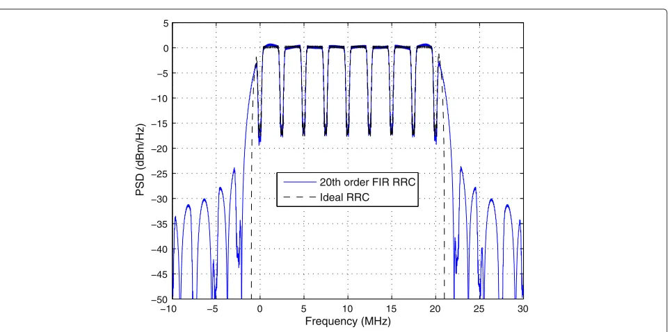
In this section, we consider the PSD and the PAPR of CB-FMT. For the OFDM system, the PSD derivation is reported in [26]. In Figure 7, we report an example of PSD of CB-FMT assuming the parameters equal toK =8,
N = 10,Q = 40,L = 32 (thereforeM = 320),β = 0.2 and the cyclic prefix equal toμ = 8 samples. The inter-polation filter is a root-raised-cosine (RRC) pulse with roll-off equal to 0.1. If the interpolation pulse were ideal, i.e., the filter was a perfect low-pass filter, the out-band
Table 1 In-band/out-of-band power ratio for CB-FMT prototype pulse
M
160 320 640 1,280
K=4,N=5 50.10 61.42 69.20 70.91
K=8,N=10 33.44 50.16 61.56 69.86
K=16,N=20 27.40 33.46 50.15 61.23
K=32,N=40 23.90 27.41 33.47 50.14
emissions would be null. However, a real interpolation filter introduces out-band emissions. For the parameters specified, the ratio between the useful signal power and out-band emissions power is equal to 25.48 dB. In OFDM, assuming the number of sub-channels equal toK =320, this ratio is equal to 22.80 dB. CB-FMT has slightly better in-band/out-band power ratio due to a higher sub-channel frequency selectivity w.r.t OFDM, under comparable com-plexity assumption. If we set the number of sub-channels in OFDM equal toK = 8, then its in-band/out-of-band power ratio will decrease even further to 20.1 dB.
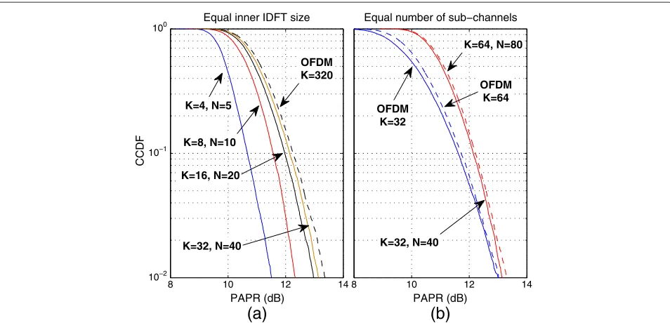
We now consider the PAPR. The complementary cumu-lative distribution function (CCDF) of the PAPR for CB-FMT and OFDM is shown in Figure 8. The PAPR is influenced by the inner IDFT block size. In Figure 8a, we perform a comparison under similar complexities, i.e., the number of sub-channels in OFDM is set equal toK=320, and in CB-FMT, we setM=320 andK∈ {4, 8, 16, 32}. In CB-FMT, the PAPR is significantly lower than in OFDM for low values ofK,N. In Figure 8b, we perform a compar-ison under an equal number of sub-channels. In CB-FMT, we keep the IDFT block size equal toM = 320. In this case, OFDM outperforms CB-FMT due to the smaller inner IDFT size. In the simulations, a 4-PSK constellation is used for both systems. As it is shown in the next section, CB-FMT can offer higher spectral efficiency than OFDM with a smaller number of sub-channels. In turn, this allows to obtain a lower PAPR.
In Table 2, the mean PAPR for CB-FMT is shown when
320 640 960 1280 0
50 100 150 200 250 300
M Conventional FMT
cop/sample
320 640 960 1280
10 12 14 16 18 20 22
M CB−FMT
K=8, N=10 K=16, N=20 K=32, N=40 K=64, N=80 OFDM, M subchan.
Figure 6Complexity of CB-FMT, FMT, and OFDM in terms of cop/sample as a function of the parameters.
than in CB-FMT for all parameter combinations herein considered.
6.4 Performance in fading channels
In order to evaluate the performance of CB-FMT, we consider the transmission over a wireless fading chan-nel. We consider both static and time-variant channels. In
particular, the channel coefficientsα(n)in (49) are mod-eled according to Clarke’s isotropic scattering model [27]. Therefore, they are assumed to be independent stationary zero-mean complex Gaussian processes with correlation defined as
Eα∗(m)α(m+n)=J0(2πfDn)δ(−), (69)
−10 −5 0 5 10 15 20 25 30
−50 −45 −40 −35 −30 −25 −20 −15 −10 −5 0 5
Frequency (MHz) PSD (dBm/Hz) 20th order FIR RRCIdeal RRC
8 10 12 14 10−2
10−1 100
Equal inner IDFT size
PAPR (dB)
(a)
CCDF
8 10 12 14
Equal number of sub−channels
PAPR (dB)
(b)
K=4, N=5
K=8, N=10
K=16, N=20
K=32, N=40
K=64, N=80
OFDM K=320
OFDM K=32
OFDM K=64
K=32, N=40
Figure 8The PAPR complementary cumulative distribution function (CCDF) for CB-FMT and OFDM.(a)PAPR when CB-FMT and OFDM have equal inner IDFT size.(b)PAPR when CB-FMT and OFDM have equal number of sub-channels. Both transmitted signals are interpolated with a 20th-order root-raised-cosine filter.
wherefD andJ0(·)are the maximum Doppler frequency and the zero-order Bessel function of the first kind, respectively. We assume an exponential power decay pro-file, i.e., = 0 e−/γ, where 0 is a normalization constant to obtain unit average power, andγ is the nor-malized, w.r.t. the sampling period, delay spread. The channel impulse response is truncated at−10 dB.
First, we show the performance in terms of average SER versus signal-to-noise ratio (SNR) varying the delay spreadγ, considering CB-FMT and OFDM both using a CP and a 1-tap MMSE equalizer at the receiver. 4-PSK modulation is assumed. Then, we show the maximum achievable data rate as a function of Doppler spread for different SNR values.
In Figure 9a, the CB-FMT system has parametersK =8,
N =10,M=320, and CP with length 8 samples. For the OFDM system, we consider the number of sub-channels equal toK=64, as in the IEEE 802.11 WLAN standard. In OFDM, the CP length is set equal to 18 samples so that the two systems have identical transmission rate assuming an identical transmission bandwidth. We consider channels
Table 2 Mean PAPR in CB-FMT for different values ofK andN
K N Mean PAPR [dB]
4 5 10.03
8 10 10.76
16 20 11.06
32 40 11.19
with normalized delay spread equal toγ = {1, 2, 3}and no Doppler spread (static channels). The results reveal that CB-FMT can significantly lower the SER, especially for high values of delay spreadγ. A 10-dB SNR gain is found at SER=10−4.
This is due to the fact that CB-FMT in conjunction with the MMSE equalizer can exploit the frequency diversity introduced by the channel, and thus, the more dispersive the channel, the higher the gain is for CB-FMT. In OFDM, the performance is identical for all values ofγ considered, since the sub-channels see flat Rayleigh fading [17].
In Figure 9b, we show the SER for several combina-tions of parameters in CB-FMT. In all cases, CB-FMT hasM = 320, K ∈ {8, 16, 32, 64}, N ∈ {10, 20, 40, 80}, and a CP equal to 8 samples so that it has the same data rate of OFDM. The normalized delay spread is set to
γ = 2. The SER grows with the number of sub-channels
K, and it approaches that of OFDM, i.e., the performance of 4-PSK in flat Rayleigh fading. This is because when
K increases, Q = M/K decreases and, consequentially, the ability of coherently capturing the sub-channel energy (thus exploiting diversity) with the MMSE equalizer is reduced.
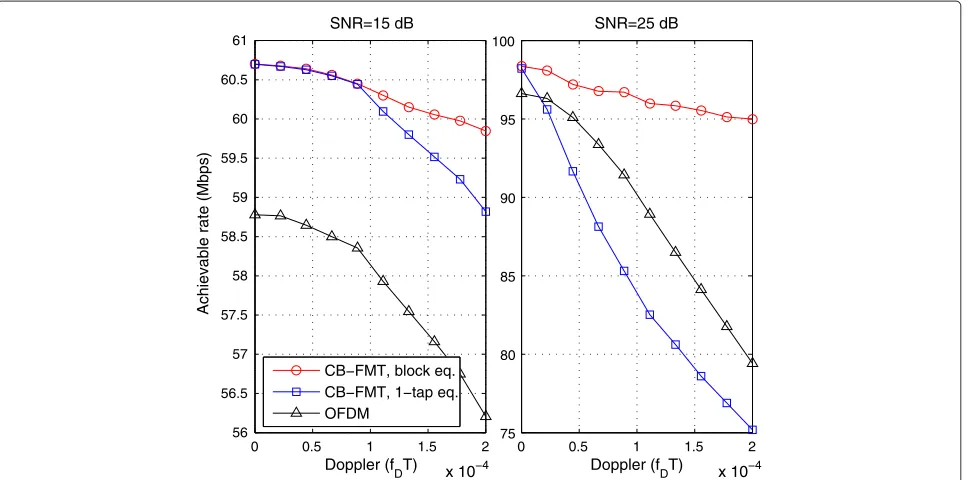
In Figure 10, we show the average maximum achiev-able rate (Shannon capacity [23]) assuming time-variant frequency-selective fading and additive white Gaussian noise. The system parameters for OFDM and CB-FMT are equal to those assumed for the SER analysis in Figure 9a. Furthermore, we assume the transmission bandwidth
0 10 20 30 40 10−7
10−6
10−6 10−5
10−5 10−4
10−4 10−3
10−3 10−2
10−2 10−1
10−1
100 100
SNR (dB)
(a)
SER
CB−FMT,γ=1 CB−FMT,γ=2 CB−FMT,γ=3 OFDM,γ ∈ {1,2,3}
0 10 20 30 40
SNR (dB)
(b)
K=8, N=10 K=16, N=20 K=32, N=40 K=64, N=80 OFDM, K=64
Figure 9Symbol error rate.(a)SER vs. SNR varying the normalized delay spreadγfor CB-FMT and OFDM.(b)SER vs. SNR for various combinations of CB-FMT parameters whenγ=2. The systems have identical transmission bandwidth and data rate.
γ = 2. For the OFDM system, we use a 1-tap MMSE sub-channel equalizer. For CB-FMT, we apply two differ-ent equalizers. Firstly, we use a 1-tap MMSE equalizer, similar to the OFDM equalizer. Then, we use the sub-channel block equalizer described in Section 5.2. For low
SNRs (equal to 15 dB in the considered case), the 1-tap equalizer in CB-FMT is sufficient and provides good per-formance which is better than that offered by OFDM also in the presence of high Doppler spreads. For high SNRs (25 dB in the considered case), CB-FMT with single-tap
0 0.5 1 1.5 2
x 10−4 56
56.5 57 57.5 58 58.5 59 59.5 60 60.5 61
Achievable rate (Mbps)
Doppler (f
DT) Doppler (fDT) x 10−4
SNR=15 dB
0 0.5 1 1.5 2
75 80 85 90 95 100
SNR=25 dB
CB−FMT, block eq. CB−FMT, 1−tap eq. OFDM
equalization provides higher achievable rate than OFDM for a Doppler below 400 Hz. For higher Doppler, the per-formance is dominated by the interference. Therefore, the MMSE sub-channel block equalizer provides significantly higher performance than the single-tap equalizer. In par-ticular, at the maximum Doppler considered that is equal to 4 kHz, the gain in achievable rate of CB-FMT over OFDM is 6%, 20% for an SNR equal to 15 and 25 dB, respectively. This shows that CB-FMT has the potential-ity of bettering the performance of OFDM also in the presence of channel time variations introduced by mobil-ity of the nodes. The gains in Figure 10 are due to the fact that CB-FMT is more robust to the channel time variations due to the use of frequency confined pulses that allow to lower the ICI compared to OFDM. Further-more, as shown also in the BER curves, CB-FMT with the FD equalizer can exploit the sub-channel frequency diversity.
7 Conclusions
In this paper, a filter bank architecture referred to as cyclic block filtered multitone (CB-FMT) modulation is presented. This scheme can be derived from the FMT architecture philosophy. However, linear convolutions are substituted with circular convolutions, and data are pro-cessed in blocks, which justifies the acronym CB-FMT. The efficient implementation of CB-FMT in the frequency domain has been discussed, and the performance anal-ysis has been carried out. The main conclusions can be summarized as follows:
• The computational complexity analysis shows that CB-FMT can significantly lower the complexity compared to conventional FMT with even longer pulses.
• The orthogonal CB-FMT design can be done in the frequency domain, and a simple pulse design procedure can be followed by sampling in the FD a band-limited Nyquist pulse. Optimal frequency localized orthogonal pulses for CB-FMT can also be designed in the frequency domain as recently shown in [19].
• The orthogonal CB-FMT transmitted signal shows high frequency compactness and potentially lower PAPR than OFDM if a lower number of data
sub-channels is used (still offering the same or higher spectral efficiency).
• Sub-channel FD MMSE equalization provides good performance in double-selective fading channels. In particular, lower symbol error rate and higher spectral efficiency than OFDM in multipath time-variant fading channels has been found depending on the choice of parameters.
Competing interests
The authors declare that they have no competing interests.
Received: 4 December 2013 Accepted: 23 June 2014 Published: 11 July 2014
References
1. ML Doelz, ET Heald, DL Martin, Binary data transmission techniques for linear systems. Proc. IRE.45(5), 656–661 (1957)
2. JAC Bingham, Multicarrier modulation for data transmission: an idea whose time has come. IEEE Commun. Mag.31, 5–14 (1990)
3. G Cherubini, E Eleftheriou, S Olcer, Filtered multitone modulation for very high-speed digital subscribe lines. IEEE J. Sel. Areas Commun.20(5), 1016–1028 (2002)
4. AM Tonello, Asynchronous multicarrier multiple access: optimal and sub-optimal detection and decoding. Bell Labs Tech. J.7(3), 191–217 (2003)
5. AM Tonello, A concatenated multitone multiple-antenna air-interface for the asynchronous multiple-access channel. IEEE J. Selected Areas Commun.24(3), 457–469 (2006)
6. W Kozek, AF Molisch, Nonorthogonal pulseshapes for multicarrier communications in doubly dispersive channels. IEEE J. Sel. Areas Commun.16(8), 1579–1589 (1998)
7. M Harteneck, S Weiss, RW Stewart, Design of near perfect reconstruction oversampled filter banks for subband adaptive filters. IEEE Trans. Circuits Syst. II: Analog Digital Signal Process.46(8), 1081–1085 (1999) 8. B Borna, TN Davidson, Efficient design of FMT systems. IEEE Trans.
Commun.54(5), 794–797 (2006)
9. C Siclet, P Siohan, D Pinchon, Perfect reconstruction conditions and design of oversampled DFT-modulated transmultiplexer. EURASIP J. Appl. Sign. Proc.2006, 1–14 (2006)
10. N Moret, AM Tonello, Design of orthogonal filtered multitone modulation systems and comparison among efficient realizations. EURASIP J. Adv. Signal Process.2010, 1–18 (2010)
11. MV Clark, Adaptive frequency-domain equalization and diversity combining for broadband wireless communications. IEEE J. Select. Areas Commun.16(8), 1385–1395 (1998)
12. A Tonello, Method and apparatus for filtered multitone modulation using circular convolution. Patent n, UD2008A000099, WO2009135886 (2008) 13. AM Tonello, A novel multi-carrier scheme: cyclic block filtered multitone
modulation, inProc. of IEEE International Conference on Communications (ICC 2013). Budapest, 9–13 June 2013, pp. 3856–3860
14. AM Tonello, M Girotto, Cyclic block FMT modulation for communications in time-variant frequency selective fading channels, inProc. of
European Signal Processing Conference (EUSIPCO 2013). Marrakech, 9–13 Sept 2013
15. G Fettweis, M Krondorf, S Bittner, GFDM - generalized frequency division multiplexing, inIEEE 69th Vehicular Technology Conference, 2009. VTC Spring 2009. Barcelona, 26–29 Apr 2009, pp. 1–4
16. AM Tonello, Time domain and frequency domain implementations of FMT modulation architectures, inIEEE International Conference on Acoustics, Speech and Signal Processing (ICASSP 2006). vol. 4, Toulouse, 14-19 May 2006
17. AM Tonello, Performance limits for filtered multitone modulation in fading channels. IEEE Trans. Wireless Commun.4(5), 2121–2135 (2005)
18. PP Vaidyanathan,Multirate Systems and Filter Banks. Electrical Engineering. Electronic and Digital Design. (Dorling Kindersley, London, 1993) 19. M Girotto, AM Tonello, Orthogonal design of cyclic block filtered
multitone modulation, inProc. of European Wireless (EW 2014). Barcelona, 14–16 May 2014
20. AM Tonello, M Girotto, Cyclic block FMT modulation for broadband power line communications, in17th IEEE International Symposium on Power Line Communications and Its Applications (ISPLC 2013). Johannesburg, 24–27 Mar 2013, pp. 247–251
21. IEEE,802.11 Standard: Wireless LAN Medium Access Control and Physical Layer Specification. (The Institute of Electrical and Electronics Engineers, Inc., Piscataway, 2007)
24. R Van Nee, A de Wild, Reducing the peak-to-average power ratio of OFDM, inProc. of IEEE Vehicular Technology Conference (VTC 98). vol. 3, Ottawa, 18–21 May 1998, pp. 2072–2076
25. H Ochiai, H Imai, On the distribution of the peak-to-average power ratio in OFDM signals. IEEE Trans. Commun.49(2), 282–289 (2001)
26. T van Waterschoot, V Le Nir, J Duplicy, M Moonen, Analytical expressions for the power spectral density of CP-OFDM and ZP-OFDM Signals. IEEE Signal Process. Lett.17(4), 371–374 (2010)
27. GL Stuber,Principles of Mobile Communication, 2nd edn. (Kluwer, Boston, 1996)
doi:10.1186/1687-6180-2014-109
Cite this article as:Tonello and Girotto:Cyclic block filtered multitone modulation.EURASIP Journal on Advances in Signal Processing20142014:109.
Submit your manuscript to a
journal and benefi t from:
7Convenient online submission 7 Rigorous peer review
7Immediate publication on acceptance 7 Open access: articles freely available online 7High visibility within the fi eld
7 Retaining the copyright to your article