A sequential and partial ambiguity resolution strategy for improving the initialization performance of medium baseline relative positioning

(1)

FULL PAPER

A sequential and partial ambiguity

resolution strategy for improving the

initialization performance of medium-baseline

relative positioning

Shoujian Zhang, Lei Zhao

*

_{, Xintan Li and Bing Cheng}

Abstract

Ionosphere products that are relatively precise are available thanks to the efforts of the International GNSS Service (IGS), and it might be possible to obtain a high success rate for the fixed integer ambiguities for medium- or longer-baseline ambiguity resolution (AR) using the ionosphere products as a priori information constraints. In this study, we used the IGS precise ionosphere products as a priori information before forming double-difference (DD) measure-ment equations using only original observables in a mid-range relative positioning and estimated the ionosphere residuals explicitly after DD. Furthermore, we proposed a sequential and partial ambiguity resolution (SPAR) strategy under the integer least square condition to realize fast and reliable AR. To demonstrate our proposed strategy, we randomly selected seven baselines ranging from 30 to 111 km and undertook positioning in a post-processing mode using real GPS dual-frequency data. According to the results, the SPAR strategy has a faster convergence process com-pared with batch AR. For instance, the convergence time with >90 % cumulative frequency percentage (probability) for 30, 40, 56, 66, 80, 95, and 111 km baselines was advanced by 55, 50, >75, 85, >110, 65, and >35 epochs, respec-tively, with a 30-s sample interval. By considering ionospheric correction before DD, we found further improvement in the initialization performance with the use of the SPAR strategy.

Keywords: GPS, Medium-range relative positioning, Sequential and partial ambiguity resolution, Convergence time, Precise ionosphere consideration

© 2016 Zhang et al. This article is distributed under the terms of the Creative Commons Attribution 4.0 International License (http://creativecommons.org/licenses/by/4.0/), which permits unrestricted use, distribution, and reproduction in any medium, provided you give appropriate credit to the original author(s) and the source, provide a link to the Creative Commons license, and indicate if changes were made.

Background

Real-time kinematic (RTK) positioning, which is known for its precision, has been used widely as positioning technol-ogy in many fields of engineering and science. The situation is relatively simple for short-baseline (<10 km) RTK under 10 km. The double difference (DD) of satellite observables between rover and base stations mostly eliminates atmos-pheric delay errors, and the ambiguity resolution process usually employs the least squares ambiguity decorrelation adjustment (LAMBDA) method (Teunissen 1995) that is efficient in delivering reliable fixed integer ambiguities. After comparison of four ambiguity resolution (AR) methods:

LAMBDA, geometry-free models for three-carrier ambi-guity resolution (TCAR) (Forssell et al. 1997; Vollath et al. 1998), geometry-based TCAR (Teunissen et al. 2002; Feng and Li 2008, 2009), and GIF-TCAR (TCAR based on a geometry-free and ionosphere-free combination) (Wang and Rothacher 2013), Zhang and He (2015) highlighted that the LAMBDA method is optimal in both short- and medium-baseline (10–100 km) cases. Li et al. (2015) devel-oped a reliable AR strategy that efficiently resolves ambi-guities sequentially under the integer least square (ILS) condition (Teunissen 1995) for the case of short-range RTK. However, for medium or long baselines (>100 km), large ionospheric delay residuals remain after DD. The con-ventional method for overcoming this problem is to use ionosphere-free linear combinations (LCs) of the original observables and to accommodate AR using a sequential

Open Access

*Correspondence: [email protected]

(2)

rounding process of wide-lane (WL) and narrow-lane (NL) ambiguities (Takasu and Yasuda 2010). Unfortunately, the LCs of the original measurements amplify the observ-able noise and lead to the inevitobserv-able addition of positioning error. Therefore, for longer-baseline RTK, it is better to use original observables to limit the propagation of measure-ment noise. Li et al. (2014) developed efficient procedures for improved float solutions and ambiguity fixing over long-baseline RTK without using ionosphere-free measurements, although the WL AR process remained a rounding process. In fact, simple rounding schemes for WL and NL ties cannot ensure high reliability of fixed integer ambigui-ties. Teunissen (1999) provided proof that an ILS estimator of the carrier-phase ambiguities is best for maximizing the probability of correct integer estimation. Hence, the AR process should be performed under an ILS condition to ensure the reliability of the fixed integer ambiguities. Nev-ertheless, validation of the batch AR mode by the LAMBDA method might still fail because of biases in some estimated float ambiguities (Takasu and Yasuda 2010), especially in the case of long baselines. Therefore, the partial AR technique was developed, which resolves a subset of the ambiguities to overcome this condition (Teunissen et al. 1999).

Ionosphere products that are relatively precise are available owing to the efforts of the International GNSS Service (IGS), and it might be possible to obtain a high success rate for the fixed integer ambiguities for medium- or longer-baseline AR using the ionosphere products as a priori information constraints. Considering the problems mentioned above, we used the IGS precise ionosphere products as a priori information before forming the DD measurement equations using only original observa-bles in a mid-range RTK and estimated the ionosphere residuals explicitly after DD. Furthermore, we propose a sequential and partial ambiguity resolution (SPAR) strat-egy under the ILS condition to realize fast and reliable AR. In the following, we offer a detailed description of the proposed SPAR strategy. We compare the initializa-tion performances of the SPAR and batch AR strategies and investigate the influence of a priori ionosphere infor-mation on the efficiency of the SPAR strategy.

Sequential and partial ambiguity resolution (SPAR) strategy

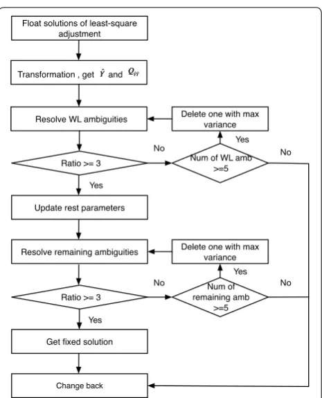
For clarity, a flowchart of this strategy is presented in Fig. 1.

After the ordinary least square adjustment stage in rel-ative positioning, we can obtain the real-value estimates and their variance–covariance matrix (dual-frequency case):

(1)

� ˆ

X Bˆ1 Bˆ2 �T

, 



Q_X_ˆ_X_ˆ Q_X_ˆ_B_ˆ₁ Q_X_ˆ_B_ˆ₂ Q_B_ˆ₁_X_ˆ Q_B_ˆ₁_B_ˆ₁ Q_B_ˆ₁_B_ˆ₂ Q_B_ˆ

2Xˆ QBˆ2Bˆ1 QBˆ2Bˆ2 

,

where B1ˆ and Bˆ2 are the DD carrier-phase ambiguity esti-mates on carrier waves L1 and L2, respectively, which should be integers, and Xˆ represents the estimates of the remaining unknowns, including the baseline components (coordinates), tropospheric parameters, and ionospheric parameters.

For medium- or longer-baseline RTK, because of the biases in some float ambiguities, batch AR by the LAMBDA method might still not pass the valida-tion step. Therefore, the partial AR technique, which resolves a subset of the ambiguities, is implemented to obtain a high success rate (Teunissen et al. 1999; Zinas et al. 2013; Wang and Feng 2013). The success rate and ratio test are different indicators with which to assess the reliability of the fixed ambiguities (Euler and Schaf-frin 1990; Teunissen 1998; Hassibi and Boyd 1998; Teunissen and Verhagen 2008; Wang and Feng 2013). The selection of the ambiguity subset, however, is not unique, and it could be based on the float ambiguity variance, elevation angle, and LCs (Mowlam and Collier 2004). Parkins (2011) described an algorithm for resolv-ing a subset of ambiguities with validation from previ-ous epochs in single-epoch RTK positioning (Wang and Feng 2013). Takasu and Yasuda (2010) employed a very

(3)

simple criterion involving the satellite elevation angle for long-baseline RTK. Li et al. (2015) chose a subset that comprised all the extra-WL or WL ambiguities in a multi-frequency case, because the extra-WL or WL ambiguities suffer relatively low effects from noise and they can be easily resolved reliably. They also indicated the possibility of resolving the ambiguities sequentially when the corresponding success rate is very close to the batch AR mode and they proposed a multi-carrier fast partial ambiguity resolution strategy that they tested with short baselines.

For longer baselines, WL ambiguity resolution will be affected inevitably by the biases in the measurements. Thus, a subset that contains all the WL float ambigui-ties without distinction might not be the best choice, and consequently, there is a need to optimize the subset. Here, we propose an optimization method that works in an iterative scheme to fix the float ambiguities with low variance. The ratio test (Euler and Schaffrin 1990) is used here for ambiguity validation. The ratio test in fact calcu-lates the closeness of the float ambiguity Bˆ to its nearest integer B¯ compared to the second nearest integer B¯′, and it reads as:

Accept B¯ if: value, to be determined by user. In general, c can be cho-sen 1.5, 2, 3 (Leick 2004; Wang and Feng 2013). In our validation step, we chose the critical value 3.

Different from the direct batch AR mode, we first con-duct a transformation:

After transformation, the ambiguity types are BˆWL and

ˆ

B1 instead of the previous B1ˆ and Bˆ2. This transformation is fundamental in our proposed strategy for introducing the WL ambiguity type.

According to the law of error propagation, the vari-ance–covariance matrix of Yˆ is:

(2)

Based on this, we propose the SPAR strategy, outlined below.

Step 1 Resolve the WL ambiguities first using the LAMBDA method; the validation technique used here is the popular ratio test with a critical threshold value of 3. Actually, this is the partial AR idea that resolves a subset of the entire float ambiguities. As the biases in the measurements have the least effect on the resolution of WL ambiguities, a subset that comprises all the WL float ambiguities is reasonable (Li et al. 2015). However, for a longer baseline, WL AR could be disturbed by measure-ment noise, meaning that it is not possible to select all the float WL ambiguities without distinction. When the validation test fails, our optimizing method deletes the float WL ambiguity with the maximum variance (which is considered the one disturbing the WL AR process) from BˆWL, and then repeats the resolution and test until

the validation test is passed, which provides the integer solution B¯WL.

Step 2 Update Xˆ, B1ˆ , and their variance–covariance matrix together with the fixed solution B¯WL. In this step,

the remaining float ambiguities on the L1 frequency and other parameters are not distinguished. The formula for the update is as below (Teunissen 1995):

Step 3 Resolve the remaining ambiguities on the L1 fre-quency using the LAMBDA method and repeat the entire process from Step 1 to obtain the remaining inte-ger ambiguities B1¯ .

Step 4 Obtain the fixed solution of the remaining unknowns using the formulas below:

Step 5 Change back. Conduct the inverse transformation of (3).

The fundamental concepts of this strategy involve resolving the WL ambiguities and the ambiguities on the L1 frequency sequentially, and optimizing the selected

(4)

ambiguity subset circularly based on the estimated ambiguity variance, as long as the validation test fails.

Experiment demonstration

Figure 2 displays the distribution of our experimental stations. We randomly selected seven baselines of the EUREF Permanent Network (EPN) and used their 3-day GPS dual-frequency observational data with a 30-s sam-pling interval, starting from day-of-year (DOY) 152 to DOY 154 in 2015. The detailed information of the data is presented in Table 1.

In the positioning process, we tested our strategy in a post-processing mode. We estimated the residual iono-spheric and tropoiono-spheric delay errors explicitly after determining the DD of the satellite observables between the rover and base stations. The relative positioning sys-tem was reset every 2 h to obtain a sufficient number of initialization samples; thus, there were almost 36 ini-tializations for each baseline during the study period. For each initialization, we were interested in the corre-sponding convergence time. A simple representation of the convergence time adopted here is the time (measured in epochs) at which no less than 90 % of the ambiguities are resolved, with the restriction that the components of the positioning errors are <10 cm. Because of noise in the observations, these 36 initializations do not perform consistently. Therefore, for both the batch AR and SPAR

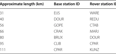
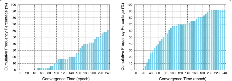
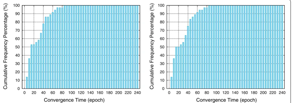
strategies, we drew pictures of the cumulative distribu-tion histograms of the convergence time corresponding to the 36 initializations of one baseline (Figs. 3, 4, 5, 6, 7, 8, 9).

It is obvious that the SPAR strategy demonstrates amazing efficiency. Taking the 31-km baseline as an example, it can be seen that the cumulative frequency percentage (probability) of the convergence time under 55 epochs is >90 % when using the SPAR strategy. Con-versely, under the batch AR strategy, the probability of the convergence time under 55 epochs is only 50 % and actually 110 epochs are needed to achieve the probabil-ity of the convergence time of >90 %. For each baseline, we recorded the corresponding convergence time when the probability in the cumulative distribution histogram was >90 % for both strategies and the results are listed in Table 2. It can be seen that the SPAR strategy is always faster than the batch AR strategy. Interestingly, for the baselines GOPE–CTAB, BRUX–DOUR, and CPAR– KUNZ, the probabilities of the convergence time are all <90 % during the 2-h interval purposely designed in our program when using the batch AR strategy, whereas the probabilities of the convergence time are all >90 % when using the SPAR strategy, corresponding to 165, 130, and 205 epochs, respectively. We speculate that this is mainly due to the large ionosphere delay residuals after DD in the case of these baselines. Since SPAR strategy inherently suffers relatively low effect in the biases of observables, it will perform still faster even toward large ionosphere residuals.

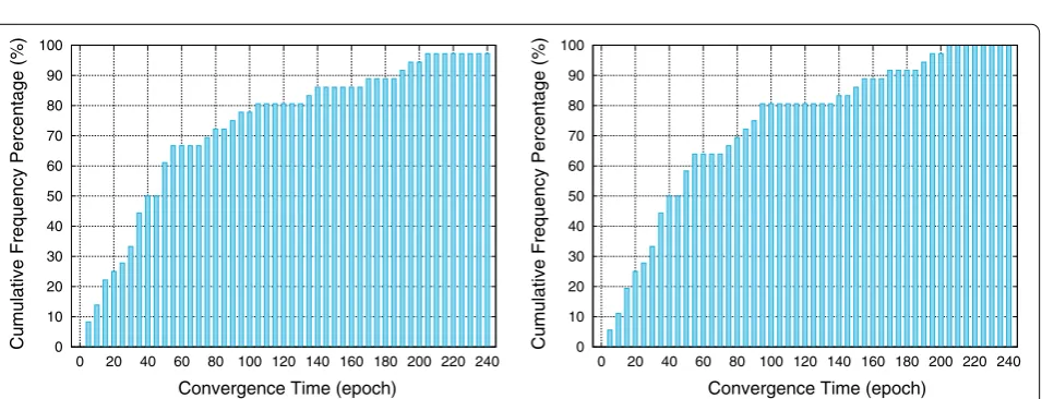
Currently, relatively precise ionosphere products are available owing to the efforts of the IGS, and it is possible to obtain a high success rate for the fixed integer ambi-guities for medium- or longer-baseline AR using the ionosphere products as a priori information constraints in a post-processing mode. Therefore, we considered performing the ionosphere correction first to further reduce the ionospheric delay errors and then to esti-mate the ionosphere residuals explicitly in the DD equa-tions. We applied two ionosphere models: the broadcast ionosphere model and the precise IGS ionosphere ver-tical total electron content (TEC) products which is in ionosphere exchange (IONEX) format to former seven baselines and performed the experiment again using the proposed SPAR strategy. The cumulative distribution histograms of the convergence time for both models are presented in Figs. 10, 11, 12, 13, 14, 15, and 16. Again, we recorded the convergence time when the probabil-ity in the cumulative distribution histogram was >90 % and the results are listed in Table 2. For the baseline of 31 km, there appears to be no improvement in the con-vergence time after considering the ionosphere correc-tion. This is because the DD operation eliminates most Fig. 2 Station distribution

Table 1 Information of selected baselines in EUREF Approximate length (km) Base station ID Rover station ID

31 EIJS WARE

40 DOUR REDU

56 GOPE CTAB

66 CRAK MARJ

80 BRUX DOUR

95 CLIB CPAR

(5)

0

Convergence Time (epoch)

0

Fig. 3 Cumulative distribution histograms of the convergence time for EIJS–WARE (30 km) baseline: (left) batch ambiguity resolution strategy and (right) sequential and partial ambiguity resolution strategy

0

Fig. 4 Cumulative distribution histograms of the convergence time for DOUR–REDU (40 km) baseline: (left) batch ambiguity resolution strategy and (right) sequential and partial ambiguity resolution strategy

0

(6)

0

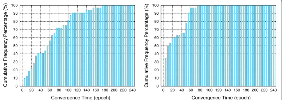
Fig. 6 Cumulative distribution histograms of the convergence time for CRAK–MARJ (66 km) baseline: (left) batch ambiguity resolution strategy and (right) sequential and partial ambiguity resolution strategy

0

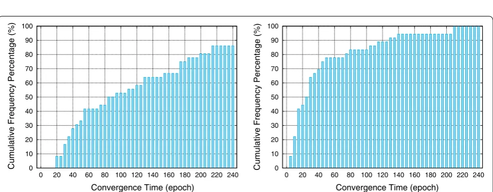
Fig. 7 Cumulative distribution histograms of the convergence time for BRUX–DOUR (80 km) baseline: (left) batch ambiguity resolution strategy and (right) sequential and partial ambiguity resolution strategy

0

(7)

of the ionospheric delay errors, which makes the correc-tion redundant at this relatively short range. However, for longer baselines, dramatic improvements in the con-vergence time can be seen. For instance, the concon-vergence time with >90 % cumulative frequency percentage is only 75 epochs for the baseline BRUX–DOUR (80 km), after applying the ionosphere correction models in the SPAR strategy, which is a considerable improvement on the original 130 epochs. But for the baseline GOPE–CTAB (56 km), broadcast ionosphere model correction seems not to bring improvement on the convergence time. We think this probably results from the low precision in the broadcast model. Interestingly, there appears to be no obvious difference between the two ionosphere models applied in the SPAR strategy for these baselines, except the 56 km and the 111 km baselines. From the 0

0

Fig. 9 Cumulative distribution histograms of the convergence time for CPAR–KUZE (111 km) baseline: (left) batch ambiguity resolution strategy and (right) sequential and partial ambiguity resolution strategy

Table 2 Comparison of initialization performance for the two strategies and comparison of initialization performance for two ionosphere correction models applied in SPAR strategy

Baseline length (km)

Convergence time (epoch) with cumu-lative frequency percentage ≥90 %

Convergence time (epoch) with cumulative frequency percentage ≥90 % for SPAR strategy

Batch AR SPAR Broadcast

model IONEX TEC model

31 110 55 55 55

40 130 80 60 60

56 >240 165 175 160

66 230 145 110 110

80 >240 130 75 75

95 130 65 60 60

111 >240 205 190 170

0

(8)

0

Fig. 11 Cumulative distribution histograms of the convergence time for DOUR–REDU (40 km) baseline: (left) broadcast ionosphere model correc-tion and (right) IONEX TEC model correction in sequential and partial ambiguity resolution strategy

0

Fig. 12 Cumulative distribution histograms of the convergence time for GOPE–CTAB (56 km) baseline: (left) broadcast ionosphere model correction and (right) IONEX TEC model correction in sequential and partial ambiguity resolution strategy

0

(9)

0

Fig. 14 Cumulative distribution histograms of the convergence time for BRUX–DOUR (80 km) baseline: (left) broadcast ionosphere model correc-tion and (right) IONEX TEC model correction in sequential and partial ambiguity resolution strategy

0

Fig. 15 Cumulative distribution histograms of the convergence time for CLIB–CPAR (95 km) baseline: (left) broadcast ionosphere model correction and (right) IONEX TEC model correction in sequential and partial ambiguity resolution strategy

0

(10)

convergence time results of the GOPE–CTAB (56 km) and the CPAR–KUNZ (111 km) baselines, it seems that the more precise IONEX TEC model leads to faster AR in comparison with the broadcast model when using our SPAR strategy.

Conclusions

In this work, we proposed a SPAR strategy for a dual-fre-quency case with estimation of atmosphere residuals for medium- and longer-baseline relative positioning. The fundamental concepts of this strategy involve resolving the WL ambiguities and the ambiguities on the L1 fre-quency sequentially, and optimizing the selected ambi-guity subset circularly based on the estimated ambiambi-guity variance, as long as the validation test fails. Tested using real GPS dual-frequency data of seven mid-range base-lines in a post-processing mode, our strategy was shown always to be faster than the batch AR mode. The conver-gence time with >90 % cumulative frequency percentage in our samples for randomly chosen 30, 40, 56, 66, 80, 95, and 111 km baselines was advanced by 55, 50, >75, 85, >110, 65, and >35 epochs, respectively, with a 30-s sample interval. We undertook ionosphere corrections for each baseline before considering the DD of the satel-lite observables with the intention of reducing the ion-ospheric delay errors further. The results showed that after considering ionosphere correction, our proposed strategy worked faster; however, differences between the ionosphere models applied with our strategy were not obvious, which means it is acceptable to use the broad-cast model with our SPAR strategy in such mid-range circumstances. Further investigation is necessary to do to test our proposed strategy in different positioning modes.

Authors’ contributions

All the authors contributed to the design of the proposed algorithm. SZ came up with the idea of partial optimization in the algorithm. XL and BC partici-pated in the experimental analysis. LZ carried out the experiments and drafted the manuscript. All authors read and approved the final manuscript.

Acknowledgements

This work is supported by Grants from the National Natural Science Founda-tion of China (Nos. 41304027 and 41274033) and the NaFounda-tional Basic Research Program of China (973 Program) (Grant No. 2013CB733301). The authors are also very grateful to the open source software RTKLIB and EPN for providing GPS dual-frequency data.

Competing interests

The authors declare that they have no competing interests.

Received: 30 November 2015 Accepted: 11 February 2016

References

Euler HJ, Schaffrin B (1990) On a measure for the discernibility between dif-ferent ambiguity solutions in the static-kinematic GPS-mode. In: Paper presented at the IAG Symposia no. 107, Kinematic Systems in Geodesy, Surveying, and Remote Sensing. Springer, New York, pp 285–295 Feng Y, Li B (2008) A benefit of multiple carrier GNSS signals: regional scale

network-based RTK with doubled inter-station distances. J Spat Sci 53(2):135–148

Feng Y, Li B (2009) Three carrier ambiguity resolutions: generalised problems, models and solutions. J Glob Position Syst 8(2):115–123

Forssell B, Martin-Neira M, Harris R (1997) Carrier phase ambiguity resolution in GNSS-2. In: Proceedings of the ION GPS-1997, Institute of Navigation, Kansas City, MO, pp 1727–1736

Hassibi A, Boyd S (1998) Integer parameter estimation in linear models with applications to GPS. IEEE Trans Signal Process 46(11):2938–2952 Leick A (2004) GPS satellite surveying, 3rd edn. Wiley, New York

Li B, Shen Y, Feng Y, Gao W, Yang L (2014) GNSS ambiguity resolution with con-trollable failure rate for long baseline network RTK. J Geod 88(2):99–112. doi:10.1007/s00190-013-0670-z

Li J, Yang Y, Xu J, He H, Guo H (2015) GNSS multi-carrier fast partial ambiguity resolution strategy tested with real BDS/GPS dual- and triple-frequency observations. GPS Solut 19(1):5–13

Mowlam AP, Collier PA (2004) Fast ambiguity resolution performance using par-tially fixed multi-GNSS phase observations. In: Paper presented at the 2004 international symposium on GNSS/GPS, Sydney, Australia, 6–8 December Parkins A (2011) Increasing GNSS RTK availability with a new single-epoch

batch partial ambiguity resolution algorithm. GPS Solut 15(4):391–402. doi:10.1007/s10291-010-0198-0

Takasu T, Yasuda A (2010) Kalman-filter-based integer ambiguity resolution strategy for long-baseline RTK with ionosphere and troposphere estima-tion. In: Proceedings of international technical meeting of the satellite Division of the Institute of Navigation, vol 7672, no 6, pp161–171 Teunissen PJG (1995) The least-squares ambiguity decorrelation adjustment: a

method for fast GPS integer ambiguity estimation. J Geod 70(1–2):65–82 Teunissen PJG (1998) Success probability of integer GPS ambiguity rounding

and bootstrapping. J Geod 72(10):606–612

Teunissen PJG (1999) An optimality property of the integer least squares estimator. J Geod 73(11):587–593

Teunissen PJG, Verhagen S (2008) GNSS ambiguity resolution: when and how to fix or not to fix? In: VI Hotine-Marussi symposium on theoretical and computational geodesy: challenge and role of modern geodesy, Wuhan, China, 29 May to 2 June 2006, Series: International Association of Geod-esy Symposia, vol 132, pp 143–148

Teunissen PJG, Joosten P, Tiberius C (1999) Geometry-free ambiguity success rates in case of partial fixing. In: Proceedings of the 1999 national techni-cal meeting of the Institute of Navigation, San Diego, CA, January 25–27, 1999, pp 201–207

Teunissen PJG, Joosten P, Tiberius C (2002) A comparison of TCAR, CIR, and lambda GNSS ambiguity resolution. In: Proceedings of the ION GPS-2002, Institute of Navigation, Portland, OR, pp 2799–2808

Vollath U, Birnbach S, Landau H, Freile-Ordonez JM, Martin-Neira M (1998) Analysis of three-carrier ambiguity resolution (TCAR) technique for pre-cise relative positioning in GNSS-2. In: Proceedings of the ION GPS-1998, Institute of Navigation, Nashville, TN, pp 417–426

Wang J, Feng Y (2013) Reliability of partial ambiguity fixing with multiple GNSS constellations. J Geod 87:1–14

Wang K, Rothacher M (2013) Ambiguity resolution for triple-frequency geometry-free and ionosphere-free combination tested with real data. J

Geod 87(6):539–553. doi:10.1007/s00190-013-0630-7

Zhang X, He X (2015) Performance analysis of triple-frequency

ambigu-ity resolution with Beidou observations. GPS Solut. doi:10.1007/

s10291-014-0434-0

Zinas N, Parkins A, Ziebart M (2013) Improved network-based single-epoch ambiguity resolution using centralized GNSS network processing. GPS