A Statistical Framework for Quantitative Trait Mapping
S´aunak Sen and Gary A. Churchill
The Jackson Laboratory, Bar Harbor, Maine 04609
Manuscript received July 29, 2000 Accepted for publication June 4, 2001
ABSTRACT
We describe a general statistical framework for the genetic analysis of quantitative trait data in inbred line crosses. Our main result is based on the observation that, by conditioning on the unobserved QTL genotypes, the problem can be split into two statistically independent and manageable parts. The first part involves only the relationship between the QTL and the phenotype. The second part involves only the location of the QTL in the genome. We developed a simple Monte Carlo algorithm to implement Bayesian QTL analysis. This algorithm simulates multiple versions of complete genotype information on a genomewide grid of locations using information in the marker genotype data. Weights are assigned to the simulated genotypes to capture information in the phenotype data. The weighted complete genotypes are used to approximate quantities needed for statistical inference of QTL locations and effect sizes. One advantage of this approach is that only the weights are recomputed as the analyst considers different candidate models. This device allows the analyst to focus on modeling and model comparisons. The proposed framework can accommodate multiple interacting QTL, nonnormal and multivariate phenotypes, covariates, missing genotype data, and genotyping errors in any type of inbred line cross. A software tool implementing this procedure is available. We demonstrate our approach to QTL analysis using data from a mouse backcross population that is segregating multiple interacting QTL associated with salt-induced hypertension.
T
HE problem of identifying the genetic factors un- QTL models because of their ability to separate linked QTL on the same chromosome and to detect interact-derlying complex and quantitative traits has a longhistory. The idea of using the association between a ing QTL that may otherwise be undetected. They pro-vide increased power to detect QTL and can eliminate discrete trait (marker) and a continuously variable
phe-notype to establish linkage of a quantitative trait locus biases in estimates of effect size and location that can be introduced by using an inappropriate single-QTL (QTL) first appeared in the work ofSax (1923). The
first known statistical approach is due toThoday(1961). model (Schork et al. 1993). A variety of approaches have been proposed for mapping multiple QTL.Haley
Modern analysis of quantitative trait genetics utilizes
andKnott (1992) described a simple approximation large sets of DNA-based markers to carry out genome
to interval mapping that is based on regression, which scans that are capable of identifying multiple genetic
can be applied to multiple-QTL models. Composite factors associated with a trait in a mapping population.
interval mapping (CIM) and multiple-QTL mapping Statistical analysis of QTL mapping data is typically
car-(MQM; Jansen 1993; Jansen and Stam 1994; Zeng
ried out by interval mapping (Landerand Botstein
1993, 1994) represent attempts to reduce the multidi-1989) in which likelihood-ratio tests are computed on
mensional search for QTL to a series of one-dimensional a dense grid of possible QTL locations. The interval
searches. This is achieved by conditioning on markers mapping procedure is based on an
expectation-maximi-outside a region of interest to account for the effects zation (EM) algorithm (Dempster et al. 1977), which
of other QTL. Multiple interval mapping (MIM) pro-maximizes the likelihood of a single-gene genetic model
posed by Kao et al. (1999) extends interval mapping by averaging over the possible states of the unknown
directly to the case of multiple QTL. An EM algorithm genotype at each possible QTL location. Despite its
ex-is used to calculate LOD scores under a multiple-QTL plicit use of a single gene model, this approach has
model. Like MIM we use an explicit multiple-QTL been successfully applied to detect multiple genes that
model but we replace the EM algorithm with a Monte underlie a wide range of complex and/or quantitative
Carlo algorithm. Thus we trade off exact computation traits.Rapp(2000) provides an excellent review of the
for ease of computation and flexibility. state of the art of QTL methodology focusing on
hyper-For pragmatic reasons, we chose to approach the prob-tension in rats.
lem of mapping multiple QTLs from a Bayesian perspec-Multiple-QTL models are an improvement over
single-tive. The Bayesian framework provides a clear picture of the probabilistic structure of the QTL mapping prob-lem. In particular, the treatment of unknown quantities
Corresponding author:Gary Churchill, The Jackson Laboratory, 600
Main St., Bar Harbor, ME 04609. E-mail: [email protected] (the QTL locations, the QTL genotypes, and the
typic means and variances) is straightforward. However, ues for a phenotype, it is implicit that there is a genetic basis for the difference. Association between the geno-we depart from a strictly Bayesian analysis at several
points as indicated below. Bayesian approaches to link- types and phenotypes in progeny derived from a cross between such strains will provide information about the age analysis and QTL mapping have been described by
others (Hoeschele andVanRaden 1993; Satagopan genetic basis for the trait. However, there are at least two components of “noise” in the data that can obscure
et al. 1996; Uimari and Hoeschele 1997; Sillanpa¨a¨
and Arjas 1999). We restrict our attention to inbred the genetic effects. First is the environmental variation that is inherent in most quantitative phenotypes. Second line crosses and comment onSatagopanet al.(1996).
They constructed a Markov chain Monte Carlo (MCMC) is the incomplete nature of the genotype information, which can only be observed at the typed markers. algorithm that sequentially samples from the unknown
QTL locations, QTL genotypes, and genetic model pa- Marker genotypes may also contain missing values and errors. Typically, an investigator is interested in knowing rameters. An advantage of the MCMC approach is the
ability to explore the model space by allowing the num- how many genes contribute to the trait, where they are located, and how they act. Statistical approaches are ber of QTL to change as part of the Markov chain
(Green1995). Our computations rely on an indepen- needed to address these questions.
Consider the simple case in which the trait is affected dent sample Monte Carlo approach, using importance
sampling of multiple imputed data sets. This avoids the by allelic variation at a single gene. In the presence of environmental variation, the phenotype can be viewed problematic issue of mixing of the Markov chain.
Fur-thermore the Monte Carlo error is inversely propor- as a “noisy” version of a biallelic locus (the QTL) whose position in the genome is unknown. If the genotype of tional to the square root of the number of imputed
data sets and can be tightly controlled. The operational the QTL could be known, the effects of the QTL could be estimated by simply looking at the distribution of simplicity of our algorithm should make it more
accessi-ble to nonspecialists in MCMC methodology. phenotypes within the groups of individuals defined by
the QTL alleles. Furthermore, the QTL position could Central to our approach is the observation that, by
conditioning on the unobserved QTL genotypes, the be localized by mapping the biallelic QTL relative to the typed markers. Thus the unknown QTL genotypes problem of QTL mapping can be divided into two
simple and statistically independent parts: the genetic are key.
If we have complete genotype information on a dense model part, which relates the QTL genotypes to the
phenotype, and the linkage part, in which the locations set of markers, a one-dimensional genome scan can be performed by regressing the phenotype on each of the of the QTL are determined. This observation is not new
(Jansen1993;Thompson2000); it is implicit in almost markers. The more a marker explains the phenotypic variance, the more likely it is to be close to a QTL. This all published work on QTL. However, making the QTL
genotypes the central focus offers several advantages. It belief can be quantified by plotting the LOD score or
F-statistic obtained from regressing the phenotype on leads to a readily implemented algorithm and that
admits a broad range of generalizations. The problems the marker. In practice the markers may be widely spaced across the genome and some marker genotypes of missing marker data, genotyping errors, covariates,
nonnormal and multivariate phenotypes, epistatic QTL, will be missing or in error. Still we can imagine having access to a dense set of completely genotyped markers; crossover interference, and nonstandard cross designs
can all be addressed within this framework. we call them pseudomarkers.Using linkage information
in the available marker data we can infer the genotypes In the sections that follow, we outline our approach
using a general notation that highlights the probabilistic of the pseudomarkers. There will be some uncertainty regarding the pseudomarker genotypes so we may de-structure of the QTL mapping problem. This de-structure
is used to devise an efficient computational strategy for cide to construct several, say 10, versions of this ideal genotype data each of which is consistent with the ob-Bayesian inference. We point out the relationship of
the log posterior distribution of QTL location (LPD) served marker genotypes. Variation in the imputed ge-notypes reflects the uncertainty in our knowledge of to the LOD score and show how the former leads to a
simple method for constructing confidence regions for the true complete genotypes. If the typed markers are dense, the variation will be negligible. As in the case QTL locations. This is followed by a description of our
software tools. After discussing possible variations of when we had complete genotype information, we can now regress the phenotype on each of the pseudomark-the basic pseudomark-theme, we demonstrate our approach with an
example of a complete QTL data analysis. Many of the ers and repeat this process for each of the imputed versions. We now have not 1, but 10 sets of LOD scores. technical details can be found inappendices a–f.
The strength of evidence in favor of a QTL being near any given pseudomarker can be quantified by averaging
A FRAMEWORK FOR QTL INFERENCE
the 10 LOD scores. For technical reasons explained below, the average is not an arithmetic mean of the Heuristic and motivation:If two inbred strains raised
This approach extends to the simultaneous mapping of multiple QTL. Suppose that there are two QTL influ-encing the trait. Using the same pseudomarkers, LOD scores are computed for eachpairof pseudomarkers for a two-dimensional genome scan. Interactions between QTL can be accommodated. We implemented pairwise and triplet genome scans and illustrate their application below. Higher-order genome scans could become
com-Figure1.—Graph of the stochastic dependencies between
putationally prohibitive. We argue below that the
pair-the five main data structures on pair-the QTL mapping problem.
wise scans should be sufficient for the analysis of data Boxes represent observed data structures and circles represent with many segregating QTL provided that interactions unobserved (or missing) data structures.
are limited to pairwise effects and that there are no groups of three or more tightly linked QTL. When these conditions are met, the results of single and pairwise
Imputed genotypes can also be used to compute the genome scans can be combined into a single statistical
marginal probability of the datapH(m,y), which is useful model that describes the simultaneous effects of
multi-for making model comparisons. ple QTL on a quantitative phenotype. The last step
To develop our arguments we begin by looking at the represents a compromise that is necessary because a
joint distribution of all of the observed and unobserved full search for four or more QTL is computationally
data. Under the assumption of no ascertainment, the impractical. The best approach to search for multiple
joint distribution can be factorized as QTL models remains an open problem.
Data structures and notation: Suppose that we have p(y,m,g,,␥)⫽
共
p(y|g,)p()兲共
p(g|m,␥)p(m)p(␥)兲
. data onnanimals or plants derived from an inbred line(1) cross. Denote the quantitative trait measurements by
A proof is provided inappendix a. This factorization
y⫽ (y1,y2, . . . ,yn)⬘, and denote the genotyping data
implies that, conditional on the QTL genotypes,g, the by then⫻kmatrixm⫽(mij), where the rows correspond
genetic model part of the problem involving (y,) can to individuals and the columns correspond to markers.
be solved independently from the linkage part of the The quantitiesyandmare theobserved data.Assume that
problem involving (m,␥). Figure 1 represents this condi-the chromosome of origin, order, and genetic distance
tional independence and highlights the central role of between the markers is known. In practice, these
quanti-the unobserved QTL genotypes. ties may have to be estimated.
This decomposition of the problem into two parts The genetic model, denoted byH, is a description of
conditional on the unobserved QTL genotypes suggests the distribution of phenotypes given the QTL
geno-that we should begin by obtaining the posterior distribu-types. If there are p contributing QTL and the trait
tion of the QTL genotypes. Inappendix bwe show that values are normally distributed within the QTL
geno-the posterior distribution of geno-the QTL genotypes after type classes, a general linear model may be used to
integrating out the parametersand␥can be expressed describe the relationship of the phenotype to the QTL
as genotypes. The parameters of the genetic model are denoted by. The locations of the QTL are denoted
p(g|y,m)⬀p(y|g)p(g|m). (2) by thep-dimensional vector␥. The QTL genotypes are
denoted by then ⫻ p matrix g⫽ (gij). The rows of g The first term indicates how compatible a phenotype is with the QTL genotypes. The second term measures the correspond to individuals and columns correspond to
the loci. The quantities,␥, andg are the unobserved compatibility of the QTL genotypes with the observed marker data.
data.Note that the meaning and dimensionality of the
unobserved data structures depend on the genetic Sampling QTL genotypes:Expression (2) suggests an
efficient computational approach for simulating from model,H.
Theory: Our goal is to make inferences about the the posterior distribution of the QTL genotypes. We can first simulate samples fromp(g|m) and then weight genetic model parameters () and the QTL locations
(␥) given the observed data. We use Bayesian statistical each sampled genotype by p(y|g). The idea is that the genotypes that are most compatible with the observed theory because it provides a convenient and
mathemati-cally consistent method for describing uncertainties in marker data are most likely to turn up in the simulation fromp(g|m). Among those genotypes, the ones that are the form of posterior distributions. As outlined above,
we combine information from the marker genotypes most compatible with the phenotypes will get the largest weights. Details are provided inappendix b.
and the phenotypes to reconstruct the unknown QTL
genotypes. Multiple imputed versions of the QTL geno- We want to consider models with multiple QTL, in-cluding cases in which there is linkage and/or interac-types are then used to compute approximations to the
the location ␥ will have p components and the QTL p(␥ ⫽u|y,m)⬀
冮
p(y|g)p(g|m,␥ ⫽u)p(␥ ⫽u)dggenotypes will constitute ann⫻pmatrix. Furthermore,
the locations are not knowna prioriand thus we want ⯝
兺
q
i⫽1
WH(ri(u)). (4)
to scan through all possible locations to search for QTL.
These considerations suggest that we should simulate In interval mapping, inference about QTL locations genotypes at all possible locations in the genome from is based on a likelihood-ratio test, which when expressed their joint distribution given the marker data. In prac- on the scale of base 10 logarithm, is called the LOD tice we generate genotypes on a discrete grid of loca- score. The LOD score at location␥can be shown to be tions spanning the genome, which we refer to as the equal to
pseudomarker grid. For a given p-tuple of
pseudo-LOD(␥)⫽constant⫹ log10
冢
sup p(y,m|,␥)
冣
. (5) marker locationsu ⫽(u1, . . . ,up), the ith realizationof genotypes is ann⫻pmatrix denoted as ri(u).
The logarithm (base 10) of the posterior distribution A weighted sample of QTL genotypes is generated by
of the QTL locations (LPD) is the following steps:
LPD(␥)⫽log10(p(␥|y,m)) 1. Select a regularly spaced grid G of pseudomarker
locations and create q realizations of the pseu- ⫽constant⫹ log
10
冢
冮
p(y,m|,␥)p()d冣
domarkers by sampling from the distributionp(g|m,␥ ⫽G). The notation␥ ⫽Gis used to indicate that ⫹ log
10(p(␥)). (6)
the entire grid of pseudomarkers is simulated as a
We expressed the LOD score and LPD in this form to joint distribution. We assume that there is no
cross-illustrate their similarity. Details are provided in
appen-over interference and that genetic distances between
dix d.By comparing (5) and (6) we see that the LOD the markers are known. With these assumptions, a
score takes a maximum over the genetic model parame-simple Markov chain sampling scheme can be used
ters whereas the LPD carries out an averaging operation. to generate the pseudomarker genotypes (Lander
In most situations when a uniform prior on the QTL andGreen 1987).
locations is used, LOD(␥) and LPD(␥) will be approxi-2. For eachp-tuple of locationsuin each pseudomarker
mately equal to each other up to an additive constant. In realization (i⫽1, . . . ,q), calculate the weight under
Figure 2, on the basis of the hypertension data discussed the assumed genetic modelH:
below, we compare the LOD score, the LPD, and the
WH(ri(u))⫽p(y|g⫽ ri(u))p(␥ ⫽u). (3) HaleyandKnott(1992) approximation to the LOD score. We can see that in this example the LOD score If the prior on the QTL locations is uniform, the and the LPD are essentially indistinguishable. However, termp(␥ ⫽u) is constant for all locationsuand can we note that it is possible to construct examples where
be ignored. the two quantities differ.
The LPD raised to the power of 10 is the posterior Note that the weight function is model dependent
density of the QTL location and hence can be used to whereas the pseudomarker generation is not. This is
construct confidence intervals (Sen 1998;Dupuisand convenient for exploring the space of models as it
re-Siegmund 1999). In our implementation, the pseu-duces the amount of computation required when a new
domarker grid is discrete, and thusp(␥|m,y) is a discrete model is considered. For normally distributed data
un-probability distribution. This is a reasonable approxima-der the assumption that the prior distribution on the tion to a continuous distribution of locations provided genetic model parameters is of the order of one obser- that the grid density exceeds our ability to resolve the vation, the weights are approximately proportional to QTL locations. In practice even a very coarse grid
n⫺v/2RSS⫺n/2, wherenis the sample size,vis the model
(10 cM) is quite effective. A denser grid (2 cM) is prefer-dimension, and RSS is the residual sum of squares ob- able for localization of QTL once they have been as-tained by regressing phenotypes on the QTL genotypes. signed to a chromosome. The discrete nature of the grid Genotypes that explain more of the variation in the makes the computation of a highest posterior density phenotype get a bigger weight. Additionally, the dimen- (HPD) region straightforward. For example, on a chro-sion of the genetic model is penalized. This penalty mosome with two QTL, the weights for each pair of
becomes important when different genetic models are pseudomarkers can be normalized and ranked from
compared. A derivation of normal model weights is pro- highest to lowest. A 1 ⫺ ␣HPD region is constructed
vided inappendix c. by including the pairs with highest weights in the set
Estimating QTL locations: In appendix b we show until the sum of the weights first exceeds 1⫺ ␣. Bayesian that the posterior distribution of the QTL location is confidence intervals based on the LPD have the desired proportional to the average weight of all pseudomarker long-run frequency coverage in large samples. SeeSen
Figure 2.—Comparison of LOD score, LPD, and Haley-Knott approximation onto the LOD score on chromosome 1 of the hypertension data: (A) Plot of the LOD score calcu-lated using the EM algorithm (solid line), the LPD (dotted line), and the approximate LOD score calculated using the Haley-Knott method (dashed line). (B) Plot of the differ-ences between LPD-LOD (dot-ted line) and LPD-approximate LOD (dashed line). (C) Plot of the proportion of missing ge-notype information as a func-tion of locafunc-tion on chromo-some 1. One can see that the three methods agree with each other where the proportion of missing genotype information is small. The discrepancy in-creases as the proportion of missing information increases.
Substantive prior information can be incorporated if a chromosome is assumed to contain two QTL, we use a summation over all pairs of pseudomarkers on into the LPD through the additive term log10p(␥). This
is analogous to the process of accumulating evidence the chromosome to estimate the effects associated with the two QTL. If two unlinked QTL have an interaction by adding LOD scores (Morton1955).
Estimating QTL model parameters: In appendix b term in the model, the two must be considered simulta-neously and the summation will run over all pairs on we show that the posterior distribution of the model
parameters can be expressed as the two chromosomes of interest. By estimating the
pa-rameters associated with small subsets (of size one, two,
p(|y,m)⬀
冮冮
p(|g,y)WH(g,␥)p(g|m,␥)dg d␥ or three) separately we can significantly reduce the amount of computation with negligible effects on the⯝
兺
qi⫽1
兺
up(|y,g⫽ ri(u))WH(ri(u)), (7) results. When we are estimating effects of one set of QTL, the other QTL may be represented by including where the summation onuis over allp-tuples of pseu- marker genotypes as covariates in the regression (see domarker locations. The first term in the summation is section on covariates below) as in CIM and MQM. Alter-the “complete data” posterior distribution of Alter-the model natively, we can simply ignore the other QTL. In practice parameters given the phenotypes and the QTL geno- both approaches yield essentially identical point esti-types. The second is the weight of the QTL genoesti-types. mates. This is a consequence of the independent assort-Thus (7) is a weighted mixture of complete data poste- ment of chromosomes, which results in approximate rior densities. Posterior means and variances of the orthogonality between unlinked locations in the ge-model parameters, E(|y, m) and V(|y,m), are com- nome. The standard errors will generally be smaller puted by the method of iterated expectation as detailed when conditioning.
inappendix b. Model scanning and model selection:In practice, the
We depart from a strictly Bayesian approach here. genetic modelH, which includes the number of QTL Suppose that we are entertaining a model with six QTL. and their interactions, is not known and has to be cho-The summation overuin (7) would range over all sextu- sen on the basis of the data. The problem of selecting
ples of pseudomarkers in the genome and could be an appropriate model is challenging and we cannot
prohibitive to compute. In practice we take advantage offer a complete formal solution. The model selection of the partitioning of the genome into chromosomes. problem is fundamental to multiple QTL analysis.
Bro-We estimate the model parameters one (or two) chro- manandSpeed(1999) reviewed different QTL analysis mosomes(s) at a time and restrict the summation over methods from a model-selection point of view. They propose a criterion for model selection on the basis of
a modification of the Bayesian information criterion there is a significant interaction, the pair represents two interacting QTL. If the interaction is not significant, (BIC) ofSchwarz(1978), which they called BIC␦.Kao
et al.(1999) use a stepwise selection procedure. each member of the pair should be individually
signifi-cant. In this case the pair represents two additive QTL. The Bayes factor (KassandRaftery1995) is a
Bayes-ian inferential device that can be used to support an InSugiyamaet al.(2001) the secondary decisions were made using marker-regression-based tests and nominal exploratory analysis of potential models. The Bayes
fac-tor for comparing two models,HandK, is the ratio of Pvalues. In our application we are using Bayes factors on the chromosomes on which the loci are located. the marginal distribution of the observed data
calcu-lated under the two models Secondary decisions about the significance of the
inter-action do not require genomewide corrections as the pair has already been selected on the basis of a stringent
B(H,K)⫽pH(y,m)
pK(y,m)
. (8)
criterion. One should be reasonably conservative about declaring interaction effects. We suggest that aPvalue The marginal probability of the data under a modelH
of at least 0.01 or a Bayes factor of 10 is a reasonably is approximately equal to the average of all the
pseu-conservative guideline. domarker weights
Stepwise procedures for model selection using the BIC␦ ofBroman andSpeed (1999) and theF-to-enter pH(y|m)⯝
1
qs
兺
q
i⫽1
兺
uWH(ri(u)),
criterion ofKaoet al.(1999) can be carried out using our software tools. It is an area that holds promise but (see appendix e), where s is the number of p-tuples one we have not adequately explored. We also note of pseudomarker locations. In practice we limited the that a QTL may be deemed important if it explains a application of Bayes factors to making decisions about substantial proportion of the variance even if it fails to subsets of the QTL in a model. For example, we may achieve statistical significance.For nonnormally
distrib-compare a two-QTL model on a given chromosome uted phenotypes the ANOVA concept does not carry
to a single-QTL model on that chromosome. We can over and alternative criteria (such as those based on compare a two-QTL model with an interaction term to deviance in the case of generalized linear models) may a two-QTL model with only additive effects. In these be used. How well a QTL is localized also provides a cases, the summation onucan be restricted to the chro- measure as to how important the QTL may be. Some mosome of interest. Bayes factors can present computa- balance of judgment is required and all the evidence
tional difficulties (Satagopanet al.1996). in support of a reported QTL should be reported.
Our data analysis consists of a model scanning step Prior distributions:All Bayesian analyses depend on followed by model selection. It represents a departure prior distributions. The influence of the prior distribu-from the Bayesian approach to model selection. We tion decays with increasing sample size and, for most carry out single and pairwise genome scans and select problems, vanishes asymptotically. For sample sizes that only those regions (or pairs) that exceed stringent per- are typical in most QTL studies (50–250 individuals), mutation testing thresholds (Churchilland Doerge the prior distribution on the model parameters is not
1994). We then fit multiple gene models that include likely to have a large effect on the posterior distributions. the regions identified as being significant in the genome However, it has a more tangible impact on the Bayes scans. This approach is consistent with the idea that one factors used for model selection. For example, the Bayes should report only highly significant QTL to minimize factors are not well defined if (improper) reference false positive results (Lander and Kruglyak 1995). priors are used for the genetic model parameters. There is often some fine tuning required to determine In our analyses we used proper priors whose weight which interaction effects to include and to resolve linked is approximately equal to that of one observation. This QTL. These model comparisons may be carried out assumption leads to the penalty term of n⫺v/2 in the using Bayes factors or likelihood-ratio tests. weight function, wherevis the dimension of the genetic Permutation testing for the pairwise genome scan model (seeappendix c). Using proper priors also helps requires a bit of explanation. We are seeking pairs of loci stabilize numerical computations when the phenotypes that together contribute significantly to the observed are not normally distributed.
that can be used for preliminary analysis and manipula- Bayes factors for model comparisons are obtained from the output of the scan functions since the marginal tion of the data.
Pseudomarker generation is implemented in the distribution of the data under a genetic model is the average of the pseudomarker weights. Bayes factors are function IMPUTE, which takes marker genotypes and
map positions as input and generates a three-dimen- calculated on selected genomic regions of interest. For example, to compare a single-QTL model on chromo-sional array of imputed genotypes (the first dimension
is individuals, the second dimension is pseudomarker some 1 to a two-QTL additive model on chromosome 1, we will compare the average pseudomarker weight positions, and the third dimension is replications). This
array is used repeatedly in subsequent analysis steps. on chromosome 1 (obtained from MAINSCAN) to the average pseudomarker weight on chromosome 1 for an Weights for imputed QTL genotypes are computed
by genome scan functions. These functions can be ap- additive model (obtained from PAIRSCAN).
Model selection is carried out using the permutation plied to the whole genome or restricted to
chromo-somes of interest. A one-dimensional scan is performed tests on one-dimensional and two-dimensional scans fol-lowed by secondary tests. Loci can be “flagged” by the using the function MAINSCAN, which produces a LPD
profile assuming a single-QTL model at each pseu- functions FLAG and FLAG2. The former uses Bayes
factors for secondary tests while the latter uses likeli-domarker location. MAINSCAN will produce essentially
identical results to a Mapmaker/QTL analysis. A two- hood ratios.
For localization of a QTL or a pair of QTL, we con-dimensional scan can be carried out using PAIRSCAN.
This function assumes a two-QTL model and computes struct a dense pseudomarker grid on the chromosome and repeat the imputation and scanning steps on that the weights both with and without an interaction effect.
It scans through all pairs of marker loci and produces chromosome. Then we plot the results using LOCALIZE or PAIRLOCALIZE to plot the posterior distribution of a two-dimensional LPD profile. The functions
PLOT-MAINSCAN and PLOTPAIRSCAN are used to plot the the QTL or QTL pair.
We are currently constructing examples, including results from the scans. Traditionally, scanning functions
have plotted the LOD score. Our functions plot the analysis scripts that illustrate the steps involved in applying these software modules. Results will be posted proportion of variance explained. This is approximately
a linear multiple of the LOD score (LanderandBotstein on our web site. In our experience we find that each QTL data set is unique and requires a tailored analysis.
1989; Dupuis and Siegmund 1999) for models with
normally distributed phenotypes and it has an intuitive Thus we prefer an interactive software environment that allows the analyst to work with the data.
appeal. Permutation tests on the one-dimensional and two-dimensional scans are performed by PERMUTEST and PERMUTEST2, respectively. A three-dimensional
EXTENSIONS
scan can be performed using TRIPLESCAN. We
typi-cally restrict a triple scan to a limited number of geno- We consider two general classes of extensions to the basic framework, those that alter the genetic model and mic regions that have already been identified in the
one- and two-dimensional scans. TRIPLESCAN can be those that alter the linkage model. Changes to the ge-netic model can be implemented by programming a used to assess three-way interactions and is useful for
localizing QTL in some situations. For example, if there new weight function. Changes to the linkage model affect only the code that simulates the pseudomarker are two linked QTL, one or both of which interact with
a third unlinked QTL, a joint analysis of their effects genotypes. Modularity in software design as well as in data analysis that the framework provides is an impor-will be required to provide unbiased estimates of
loca-tion and effect sizes. Higher-dimensional scans may be tant advantage.
Extensions of the genetic model:For normally distrib-performed using the SCAN function. This function is
generally slower than ONESCAN or TWOSCAN but is uted phenotypes, the weights are based on a normal
regression model. More general distributions can be more flexible.
After the genome scans have been carried out we can accommodated by calculating the weights assuming a
generalized linear model (McCullagh and Nelder
obtain estimates of the QTL model parameters. For a
QTL that is not linked to or interacting with any other 1989). Generalized linear models have been mentioned by several authors, for exampleJansen(1993), but they QTL, the function ONEESTIMATE computes estimates
of the posterior mean and standard error of the effect do not appear to be widely used in practice. This may be due in part to the robustness of normal regression size. This function, applied on one chromosome at a
time, provides an estimate of the effect size of a QTL models but is also due to lack of readily available soft-ware tools.Shepelet al.(1998) used a Poisson regression
onthat chromosome.For linked and/or interacting QTL,
we provide functions TWOESTIMATE and THREE- model on marker loci and stepwise selection using the
BIC criterion to identify multiple loci. Implementing ESTIMATE. Scanning and estimation functions for
our software package only the weight function needs to phenotype in which some of the animals survive beyond the observation period. The data are represented as a be revised.
In general the weight function for any model is binary indicator of survival status (y1) and, for those animals that died, a time to death (y2). To reproduce
WH(y,g)⫽
冮
pH(y|g,)p()d. (9)the results ofBromanet al.(2000) we implemented the weight function
For generalized linear models, under the assumption
that the prior distribution on the genetic model parame- WH(y,g)⫽WB
H(y1,g)WNH(y2,g), (10) ters is of the order of a single observation, this works
where WB
H denotes the weight function corresponding out to be approximately
to a binomial distribution andWN
H to that of a normal distribution.
exp(⫺ dev 2 )n
⫺v/2,
In QTL experiments covariates are often collected in addition to the phenotypes of interest. The logic behind where dev ⯝⫺2 log(p(y|g, ⫽ ˆ )) ⫺ log(p( ⫽ ˆ ))
measuring covariates is to measure and adjust for envi-is the observed unscaled deviance (McCullagh and
ronmental factors that influence phenotypic
expres-Nelder 1989), ˆ is the posterior mean of, and v is
sion. These might be blocking factors in an agricultural the dimension of the genetic model. If the phenotype
field trial or cage number in a mouse cross. The covari-data follow a Poisson distribution, the weight function
ate may also be another phenotype, in which case some is
care must be exercised in the interpretation of results. We assume that there is no direct association between
WH(y,g)⫽
冢
兿
ki⫽1
nyi.i
yi!
冣
⫺1,
the QTL that affect the trait of interest and the covariate. If this is not the case, the phenotype and the covariate where k is the number of genotype classes, ni is the should be treated as a multivariate phenotype. We de-number of observations in theith class, and yi. is the note the covariate by x and any unknown parameters sum of the observations in the ith class. For binomial governing the distribution ofxare denoted by. It can
data, the weight function will be be shown by calculations similar to that inappendix a
that the appropriate weight function is
WH(y,g)⫽
冢
兿
ki⫽1
冢
mi.
yi.
冣冣
⫺1,
WH(y,g)⫽p(y|x,g)p(␥ ⫽u). (11)
wheremi.is the total of the size parameters of the bino- The practical implication of (11) is that the weights are mial observations in each group and yi. is the sum of now based on a regression analysis of the phenotype on
the observations in theith class. the covariates and the QTL genotypes.
Many complex trait studies involve measurement of The use of marker loci as covariates in QTL analysis
multiple related phenotypes. If two phenotypic mea- was suggested by Jansen (1993) and also by Zeng
surements are affected by the same set of genes, then it (1993). When analysis of a QTL is focused on a single can be more efficient to consider a multivariate analysis chromosome or other genomic region, the use of un-(JiangandZeng1995;Korolet al.1995;Roninet al. linked markers as covariates presents no difficulties. The 1999). If the phenotype is multivariate normal, then the weight function (11) is appropriate. This can be a useful
appropriate weighting scheme is device for reducing the complexity of QTL analysis by
accounting for other segregating QTL in a cross and is
WH(y,g)⫽ n⫺v/2det(S)⫺n/2,
easy to implement using our software tools. However, the use of linkedmarkers as covariates presents some whereSis the residual covariance matrix of the
multivar-iate ANOVA andvis the model dimension (appendix difficulties and may significantly reduce power. If there are multiple unlinked QTL in a cross, conditional
analy-c). Models in multivariate space are more complex and
some of the nice interpretations that apply to univariate sis of one QTL with marker covariates to control for others can be an effective strategy. When there are mul-normal phenotypes do not carry over. Although
multi-variate phenotyping comes with the promise of greater tiple linked QTL or interactions among unlinked QTL, we recommend a joint analysis of their effects.
power to detect QTL, there are some costs. Unless two
phenotypes are affected by the same biochemical path- Extensions of the linkage model:Missing marker data are common in QTL experiments, sometimes due to way, adding a phenotype into the analysis may add genes
and interactions to the list of genes affecting the (multi- difficulties with typing but also as a result of selective
genotyping. Following Rubin (1976) and Schafer
variate) phenotype. This may complicate the analysis of
complex traits where a large number of genes are known (1997) we argue that as long as the missingness mecha-nism depends on the observed data and not on the to be affecting the trait of interest. We recommend that
multivariate trait analysis be used with caution. missing data values, it does not have an impact on the posterior distributions of the parameters of interest. An interesting mutlivariate data structure is presented
or multiple imputation to take missing data into ac-count. If there is some ascertainment bias, such as if only animals with high phenotypes are collected and the rest discarded, then this assumption would be vio-lated. As a general rule the phenotype data from an entire cross should be included in the analysis even for individuals with no genotype information.
Let Rdenote the missing marker data pattern, and letmobsandmmisdenote the observed and missing marker data, respectively. It can be shown that the form of the posterior distributions of the QTL locations␥, the genetic model parameters, and the QTL genotypesg
given the observed data R, y, and mobs is unchanged. The marginal distribution of the observed data under the genetic modelHis
pH(y,mobs,R)⫽p(R|mobs,y)pH(y|mobs)p(mobs). (12)
Figure3.—Distribution of blood pressure values. The histo-gram of the blood pressures of 250 mice in the backcross
Thus to compute the Bayes factor for comparing
differ-reported inSugiyamaet al. (2001) is shown. Also displayed
ent models, we only need to calculatepH(y|mobs), other
on top of the histogram are the means and two standard
terms being independent of the model.
deviation error bars of the two parental strains. Eight mice in
Selective genotyping is a practical device for reducing the BL/6 strain and 10 mice in the A/J strain were measured. the cost of QTL mapping experiments (Lander and
Botstein 1989). For example, an investigator, after
measuring the phenotype of the animals from a cross, under a no-interference model cannot be used (Zhao may decide to genotype only the extremes. In this case, et al.1995).
the missing data pattern depends only on the observed data (the phenotypes). If the decision to genotype was
EXAMPLE
based on a phenotypey, but the trait of interest is
an-other phenotypez, then the appropriate analysis would We illustrate the application of our approach by a use a multivariate phenotype composed of (y, z). Al- reanalysis of a hypertension cross described in Sugi-though it is technically not correct to analyze z as a yamaet al.(2001). Blood pressure measurements were univariate trait when data have been selected usingy, obtained on 250 mice from a backcross between strain we do not anticipate a serious bias if the univariate C57BL/6J (high blood pressure) and strain A/J (low
analysis is used. blood pressure). We analyze blood pressure data
assum-Genotyping errors were considered byLincolnand ing a normal model. Figure 3 shows the distribution of
Lander(1992). Their formulation was based on a sim- the blood pressure of the backcross individuals com-ple model of the probability of a typing error. We note pared with the parental lines. The mean blood pressure that this falls into the missing data framework presented was ⵑ101.6 mm of Hg and the standard deviation of above and can be handled by modifying the pseu- the blood pressure wasⵑ8.4 mm of Hg. A total of 174
domarker simulation code. markers were typed. Initially only the extremes of the
Backcross and intercross designs have been widely backcross population were genotyped in a standard se-utilized in quantitative trait mapping studies. However, lective genotyping design. Following an initial analysis there are alternative approaches and there is interest of the data, additional genotyping was carried out in in developing new cross designs that might improve the regions of interest on all mice.
resolution of QTL mapping studies. Designs that utilize We used a 10-cM pseudomarker grid with 16 imputa-recombinant inbred lines, congenic or isogenic lines, tions for the initial scanning step. The model refine-repeated backcrossing, and advanced intercross lines ment and localization were done using a 2-cM pseu-are some examples (Darvasi 1998). In principle, any domarker grid with 256 imputations. The initial genome
crossing design can be accommodated into our proce- scan using MAINSCAN revealed two significant QTL
dure provided that one can simulate a pseudomarker on chromosomes 1 and 4 and a suggestive peak on
genotype conditional on observed marker data. chromosome 15. In Figure 4 the proportion of the
Figure4.—Results of one-dimension-al scan. The top shows the proportion of the variance explained as a function of QTL location. The pseudomarker spacing used was 10 cM and 16 sets of imputations were used. The two hori-zontal lines correspond to 1 and 5% criti-cal values based on 1000 permutations. Strong evidence for QTL on chromo-somes 1 and 4 and weak evidence for a QTL on chromosome 15 are indicated. There is a hint of two QTL on chromo-some 1. The bottom shows a plot of esti-mated effects and 95% confidence inter-vals based on a single-QTL model on each chromosome. The effect size is de-fined as half of the effect of substituting an A/J allele in place of a C57BL6/J allele.
the variance. The Bayes factor estimates for comparing for interacting QTL on chromosomes 7 and 15, which explainsⵑ5% of the variance over an additive model the null model of no genetic effects to a single-QTL
model are ⬍1 for all chromosomes except chromo- (the Bayes factor is 11.4). The Bayes factor indicates that the evidence for the 6⫻15 interaction is stronger somes 1, 4, and 15 (the respective values are 37.3, 1.1⫻
105, and 1.7). Figure 5 shows the result of a two-dimen- than that of the 7 ⫻ 15 interaction even though the size of the estimated effects is about the same (see Figure sional scan using two-QTL models fitted using
PAIR-SCAN. We find that the QTL on chromosomes 1 and 8). A look at the localization plots (see Figure 7) reveals that the localization information is stronger with the 4 together explainⵑ22% of the variance. There is
evi-dence for interaction between loci on chromosomes 6 6 ⫻ 15 interaction than with the 7 ⫻ 15 interaction. The combined results of these scans suggest that we and 15. The Bayes factor for interactionvs.no
interac-tion is 20.4. The interacinterac-tion explainsⵑ6% of the vari- should look closely at chromosomes 1 and 4 to deter-mine if there may be multiple QTL on either of these ance above an additive model. There is also evidence
Figure5.—Results of
Figure6.—Close-up of two-dimension-al scan on chromosomes 1, 4, 6, 7, and 15. This suggests that there may be two QTL on chromosome 1. The interaction effects between loci on chromosomes 6 and 15 and those on 7 and 15 are appar-ent in the top diagonal. This was pro-duced using 256 sets of imputations on a 2-cM pseudomarker grid.
chromosomes and that we should examine the simulta- tions detected using PAIRSCAN are sufficient to de-scribe the joint effect of these loci. The 6⫻15 interaction neous effects of loci on chromosomes 6, 7, and 15 to
sort out the nature and extent of the interactions. was reported by Sugiyama et al. (2001). The 7 ⫻ 15 interaction was not detected in their analysis, which may We carried out a TRIPLESCAN restricted to
chromo-somes 6, 7, and 15. There is no evidence for a three- be due to large intermarker spacings on chromosome 7. Now we turn our attention to chromosome 1, which way interaction among these markers. The Bayes factor
for the three-way interaction model vs. a model with showed some evidence for two QTL on the basis of the output from MAINSCAN and PAIRSCAN. The Bayes all three two-way interactions is 0.2. There is also no
evidence for an interaction between chromosomes 6 factor comparing a two-locus additive model on chro-mosome 1 to a single-locus model on chrochro-mosome 1 is and 7. Thus we conclude that the two pairwise
interac-Figure 7.—Summary of localization
the QTL mapping problem into the linkage part and the genetic model part. This decomposition is used to develop a computational strategy that uses multiple im-putations of a pseudomarker grid to approximate inte-grals needed to perform Bayesian inference. Our soft-ware provides a set of flexible extensible tools suitable for the analysis of QTL data.
The problem of model selection remains a thorny issue in theoretical statistics and presents a serious chal-lenge in the analysis of QTL data. For this reason we emphasized exploratory tools over formal model selec-tion procedures in our analysis. We provide a visual representation of two-QTL models and two-way interac-tions in the QTL mapping problem.
Most of the QTL analysis methods proposed so far have relied on linear (or generalized linear) regression models. Recently, classification and regression trees
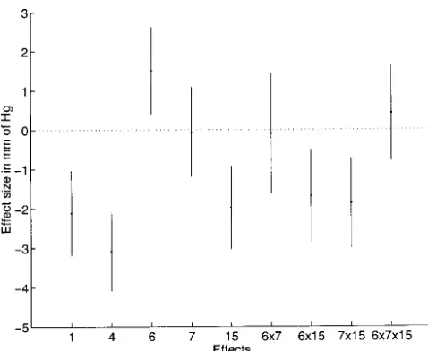
Figure8.—Estimated effects of QTL and their interactions (CART) models were proposed for QTL data (T. Speed,
in the hypertension cross. The estimated effects are identified personal communication) because they have a richer with the chromosome the QTL are in. Also shown are the
interaction space. We note here that by using
appro-95% confidence intervals for the effects based on the posterior
priate weight functions,WH(y,g), where the model,H, variances of the effects. The sizes of the interaction effects
6⫻15 and 7⫻15 are comparable to the main effects of 1 can be a regression tree, we can include CART in our
and 15. By adding up the squares of the effect sizes we find framework. that the plotted QTL effects explainⵑ41% of the total
vari-Multiple-QTL models were considered byHaleyand
ance. For comparison, we included the interaction effects 6⫻
Knott(1992), who presented a simple regression
ap-7 and 6⫻7⫻15, which are not in the final model.
proximation to the LOD score. The LOD score, the Haley-Knott approximation, and the LPD will coincide 0.41. This is inconclusive evidence but it favors the sin- at locations where there is complete genotype informa-gle-QTL model. The localization plot assuming a two- tion. At locations with incomplete genotype informa-QTL model on chromosome 1 seems to indicate two tion, the three versions of the LOD score will differ. QTL, but not overwhelmingly. Additional experimenta- This can be seen in Figure 2. The regression approxima-tion may be needed to provide stronger evidence for tion to the LOD score deviates substantially from the
the presence of two QTL on chromosome 1. We note LOD score and the LPD in regions where the
propor-thatSugiyamaet al.(2001) conclude that there are two tion of missing information is high. The bias in the
QTL on chromosome 1. Our reanalysis suggest weaker HaleyandKnott(1992) approximation to the LOD
evidence in favor of two QTL than their original analysis. score has been investigated in detail byKao (2000). A localization scan of chromosome 4 suggests the possi- We have already mentioned the close connection be-bility of multiple QTL but again there is not strong tween the LOD score and the LPD. Notwithstanding support provided by the Bayes factor, which is 0.15. their similarities, the two can be numerically divergent. The final model that we arrived at through this analy- There is an importantconceptualdifference between the sis includes five loci on chromosomes 1, 4, 6, 7, and 15. LOD score and the LPD. The LOD score is designed The localization information for these loci is given in to be atest for linkagewherein the location of the QTL Figure 7. The main effects for QTL explain, respectively, (␥) is a nuisance parameter andis the parameter of 6, 13.5, 3, 0, and 5.5% of the variance. There are two two- interest. Indeed, themaximumof the LOD score is used way interactions in the model. The interaction between as the test statistic for linkage. The LPD is designed with QTL on chromosomes 6 and 15 explainsⵑ6% and the the reciprocal purpose oflocalizationwhere the location one between QTL on chromosomes 7 and 15 explains of the QTL (␥) is the parameter of interest. The
parame-ⵑ6.5% of the variance. Taken together the model ex- teris the nuisance parameter and is integrated out. plainsⵑ41% of the variance. The effect sizes are summa- The Monte Carlo error in approximating the
poste-rized in Figure 8. rior distributions by the pseudomarker algorithm is
in-versely proportional to the square root of the number of imputations. Unlike MCMC methods, we do not have
DISCUSSION
to worry about proper mixing of the Markov chains. Accuracy of the calculations also depends on the density We analyzed the stochastic dependencies between the
different observed and unobserved data structures in of the pseudomarker grid. For initial genome scans we find that 20 pseudomarker sets at a spacing ofⵑ10 cM the QTL mapping problem. By conditioning on the
pseudomarker map on selected chromosomes with QTL mapping studies will continue to contribute to our understanding of the nature of quantitative trait
ⵑ200 replicated data sets. Adjustment for individual
situations is quite easy. More replications may be re- genetics. However, to achieve this goal we must acknowl-edge the complexity of quantitative inheritance, which quired when the proportion of missing genotypes is
high. The investigator will have to vary the density of is often determined by multiple interacting genetic loci, and we must develop and apply analytic methods that the pseudomarker map and the number of replicated
data sets according to his/her needs. The best way to are appropriate for this problem.
know what is reasonable for the map is to start with a We thank Drs. B. Paigen, F. Sugiyama, and K. Broman for sharing sparse pseudomarker set and repeat the analysis. If the data with us. This work has benefited enormously from the critical comments of Dr. K. Broman and two anonymous referees. The Ameri-pictures differ markedly, more replications are needed.
can Heart Association provided financial support through a grant to To control Monte Carlo fluctuations we also adopted
G.A.C. some additional devices explained in greater detail in
appendix f.Another option to controlling Monte Carlo noise (which we have not currently implemented)
LITERATURE CITED
would be to use smoothing techniques on the LPD since
Broman, K. W.,andT. Speed,1999 A review of methods for identi-it is approximately piecewise quadratic (Kong and
fying QTLs in experimental crosses, pp. 114–142 inStatistics in
Wright1994). The variation in the imputed genotypes Genetics and Molecular Biology, Vol. 33 of IMS Lecture Notes—
Monograph Series, edited byF. Seiller-Moiseiwitsch.Institute at a pseudomarker location can be used as an estimate
of Mathematical Statistics, Hayward, CA. of the amount of missing genotype data for that
loca-Broman, K. W., V. L. BoyartchukandW. F. Dietrich,2000 Map-tion. This may be used to decide if more genotyping ping time-to-death quantitative trait loci in a mouse cross with high survival rates. Technical Report MS00-04, Department of needs to be done in a particular region of the genome;
Biostatistics, Johns Hopkins University, Baltimore. we implemented a graphical diagnostic tool called
Churchill, G.,andR. Doerge,1994 Empirical threshold values PLOTMISSINGPROP to identify regions of the genome for quantitative trait mapping. Genetics138:963–971.
Darvasi, A.,1998 Experimental strategies for the genetic dissection that might benefit from additional genotyping.
of complex traits in animal models. Nat. Genet.18:19–24. We presented a QTL mapping framework in the
con-Dempster, A., N. LairdandD. Rubin,1977 Maximum likelihood text of analyzing data from inbred line crosses. However, from incomplete data via the EM algorithm. J. R. Stat. Soc. Ser.
B39:1–22. the idea of using multiple imputation of complete
Dupuis, J.,andD. Siegmund,1999 Statistical methods for mapping genotype information is applicable to more general
quantitative trait loci from a dense set of markers. Genetics151:
gene-mapping situations, including complex human 373–386.
Green, P.,1995 Reversible jump Markov chain Monte Carlo compu-pedigrees. How it performs in practice requires further
tation and Bayesian model determination. Biometrika82:711– investigation.
732.
Finally, it is pertinent to point out some of the inher- Haley, C.,andS. Knott,1992 A simple regression method for mapping quantitative trait loci in line crosses using flanking mark-ent limitations of QTL mapping studies. The number
ers. Heredity69:315–324. of QTL that we can reliably detect in a cross depends
Hoeschele, I.,andP. VanRaden,1993 Bayesian analysis of linkage on the number of individuals available, the numbers of between genetic markers and quantitative trait loci. II. Combining prior knowledge with experimental evidence. Theor. Appl. segregating QTL, and the strength of their effects. If
Genet.85:946–952. there are interactions between QTL that are ignored,
Jansen, R.,1993 A general mixture model for mapping quantitative then we may fail to find those QTL. For example, with trait loci by using molecular markers. Theor. Appl. Genet.85:
252–260. 100 progeny from a backcross, we can expect to observe
Jansen, R. C.,andP. Stam,1994 High resolution of quantitative
ⵑ25 individuals in each genotype class for two unlinked
traits into multiple loci via interval mapping. Genetics136:1447–
QTL. With three unlinked QTL, the number isⵑ12. If 1455.
Jiang, C.,andZ-B. Zeng, 1995 Multiple trait analysis of genetic the three QTL are linked, some genotype classes may
mapping for quantitative trait loci. Genetics140:1111–1127. be unrepresented in the data or may have very small
Kao, C.-H.,2000 On the difference between maximum likelihood numbers. Thus, it may be impossible to detect and char- and regression interval mapping in the analysis of quantitative
trait loci. Genetics156:855–865. acterize interactions of order 3 or higher and genes
Kao, C.-H., Z-B. ZengandR. D. Teasdale,1999 Multiple interval that act through high-order interactions may not be
mapping for quantitative trait loci. Genetics152:1203–1216. detected. It has been shown that model misspecification Kass, R.,andA. Raftery,1995 Bayes factors. J. Am. Stat. Assoc.90:
773–795. can lead to misleading results (Wright and Kong
Kong, A.,andF. A. Wright,1994 Asymptotic theory for gene map-1997). We also acknowledge that the localization of QTL
ping. Proc. Natl. Acad. Sci. USA91:9705–9709.
in any cross of a reasonable size is limited by the number Korol, A. B., Y. I. RoninandV. M. Kirzhner,1995 Interval mapping of quantitative trait loci employing correlated trait complexes. of crossover events. QTL mapping studies will generally
Genetics140:1137–1147. not be adequate to identify the polymorphic genes or
Lander, E.,and D. Botstein, 1989 Mapping Mendelian factors regulatory regions that are affecting a trait of interest. underlying quantitative traits using RFLP linkage maps. Genetics
121:185–199. The availability of complete genome sequences will
ex-Lander, E.,andL. Kruglyak,1995 Genetic dissection of complex pand the list of candidate genes for a QTL and will
traits: guidelines for interpreting and reporting linkage results. facilitate efforts to identify the genes responsible for the Nat. Genet.11:241–247.
netic linkage maps in humans. Proc. Natl. Acad. Sci. USA84: The first equality is an application of the definition of 2363–2367.
conditional probability and the second follows from the
Lee, P. M.,1997 Bayesian Statistics, Ed. 2. Arnold Publishers, London.
Lincoln, S. E., and E. S. Lander,1992 Systematic detection of assumption that the phenotype depends on the location errors in genetic linkage data. Genomics14:604–610. of the gene only through the genotype of the QTL and
McCullagh, P.,andJ. Nelder,1989 Generalized Linear Models, Ed.
the genetic model. The third equality follows from the 2. Chapman & Hall, London/New York.
Morton, N.,1955 Sequential tests for the detection of linkage. Am. assumption that the distribution of the QTL genotype
J. Hum. Genet.7:277–318. depends on the genetic model only through the position
Rapp, J. P.,2000 Genetic analysis of inherited hypertension in the
of the QTL relative to the markers. In the final equality rat. Physiol. Rev.80:131–172.
Ronin, Y. I., A. B. KorolandE. Nevo,1999 Single- and multiple-trait we assume that the distribution of the marker genotypes mapping analysis of linked quantitative trait loci: some asymptotic is independent of the location of the QTL and the analytical approximations. Genetics151:387–396.
disease model and regroup the terms. This final
assump-Rubin, D.,1976 Inference and missing data. Biometrika63:581–592.
Satagopan, J., B. Yandell, M. NewtonandT. Osborn,1996 A tion will be true if there is no ascertainment. If individu-Bayesian approach to detect quantitative trait loci using Markov als have been selected based on their phenotype and chain Monte Carlo. Genetics144:805–816.
the phenotypes of nonselected individuals are not
in-Sax, K.,1923 The association of size difference with seed-coat
pat-tern and pigmentation inphaseolus vulgaris.Genetics8:552–560. cluded in the analysis this result will not hold.
Schafer, J.,1997 Analysis of Incomplete Multivariate Data.Chapman & Hall, London/New York.
Schork, N., M. BoehnkeandJ. Terwilliger,1993 Two-trait-locus
APPENDIX B: POSTERIOR DISTRIBUTIONS
linkage analysis: a powerful strategy for mapping complex genetic traits. Am. J. Hum. Genet.53:1127–1136.
An expression for the distribution of the QTL
geno-Schwarz, G.,1978 Estimating the dimension of a model. Ann. Stat.
6:461–464. types given the observed data can be derived from the
Sen, S.,1998 Confidence intervals for gene location: the effect of full joint distribution using elementary operations as model misspecification and smoothing. Ph.D. Thesis,
Depart-ment of Statistics, University of Chicago. p(g|m,y)⬀
冮冮
p(y,m,g,,␥)dd␥Shepel, L. A., H. Lan, J. D. Haag, G. M. Brasic, M. E. Gheenet al., 1998 Genetic identification of multiple loci that control breast
⫽
冮
冤
冮
p(y|g,)p()d冥
cancer susceptibility in the rat. Genetics149:289–299.
Sillanpa¨a¨, M.,andE. Arjas,1999 Bayesian mapping of multiple quantitative trait loci from incomplete outbred offspring data.
⫻
冤
p(g|m,␥)p(m)p(␥)冥
d␥Genetics151:1605–1619.
Sugiyama, F., G. A. Churchill, D. C. Higgins, C. Johns, K. P.
Makaritsis et al., 2001 Concordance of murine quantitative ⬀
冮
p(y|g)p(g|m,␥)p(␥)d␥ trait loci for salt-induced hypertension with rat and human loci.Genomics71:70–77.
⫽ p(y|g)p(g|m). (B1)
Thoday, J.,1961 Location of polygenes. Nature191:368–370.
Thompson, E. A.,2000 Statistical Inference From Genetic Data on
Pedi-The expression (B1) suggests that we obtain a
represen-grees, Vol. 6 ofNSF-CBMS Regional Conference Series in Probability
and Statistics.Institute of Mathematical Statistics, Beachwood, OH. tation of the posterior distribution of g by sampling
Uimari, P., andI. Hoeschele,1997 Mapping-linked quantitative from
p(g|m, ␥) and then weighting the samples by trait loci using Bayesian analysis and Markov chain Monte Carlo
W(g) ⫽ p(y|g). The weights are importance sampling algorithms. Genetics146:735–743.
Wright, F. A.,andA. Kong,1997 Linkage mapping in experimental weights and the idea is thatp(g|m) has a flatter distribu-crosses: the robustness of single-gene models. Genetics146:417–
tion than p(g|m, y) and therefore is a good proposal 425.
distribution to use. Summing the weights is a numerical
Zeng, Z-B.,1993 Theoretical basis of separation of multiple linked
gene effects on mapping quantitative trait loci. Proc. Natl. Acad. approximation to integration with respect top(␥)d␥. It Sci. USA90:10972–10976.
is possible to use an irregularly spaced list of␥values.
Zeng, Z-B.,1994 Precision mapping of quantitative trait loci.
Genet-In that case we will have to weigh each point suitably ics136:1457–1468.
Zhao, H., T. P. SpeedandM. S. McPeek,1995 Statistical analysis as in a numerical trapezoidal integration formula. A of crossover interference using the chi-square model. Genetics
numerical integration over the QTL location space is 139:1045–1056.
reasonable because the shape of the log-likelihood in Communicating editor:S. Tavare´ large samples is piecewise quadratic and hence smooth
(KongandWright1994).
The posterior distribution of the QTL locations is
APPENDIX A: FACTORIZATION OF THE JOINT DISTRIBUTION
p(␥|m,y)⬀
冮冮
p(y,m,g,,␥)dg dThe joint distribution of the observed and missing
⫽
冮冮
p(y|g,)p()p(g|m,␥)p(m)p(␥)dg ddata structures is
p(y,m,g,,␥)⫽p(y|m,g,,␥)p(m,g,,␥) ⫽
冮
冤
冮
p(y|g,)p()d冥
p(g|m,␥)p(␥)p(m)dg (B2) ⫽p(y|g,)p(g|m,,␥)p(m,,␥)⬀
冮
p(y|g)p(g|m,␥)p(␥)dg (B3) ⫽p(y|g,)p(g|m,␥)p(m,,␥)≈
兺
qi⫽1
WH(ri(␥))p(␥). (B4)