Model development for shape memory polymers

Model Development for Shape Memory Polymers

Ryan D. Siskind

and Ralph C. Smith

Department of Mathematics

North Carolina State University, Raleigh, NC 27695

ABSTRACT

The nonlinear thermomechanical relationship in shape memory polymers (SMPs) has drawn considerable atten-tion in many fields ranging from aeronautics to medicine largely due to their ability to withstand deformaatten-tions several orders of magnitude larger than in shape memory alloys (SMAs). At high temperatures, SMPs share attributes with compliant elastomers and exhibit long-range reversibility. In contrast, at low temperatures they become very rigid and are susceptible to plastic, although recoverable, deformations.

Keywords: shape memory polymers, smart materials

1. INTRODUCTION

Whereas the research involving shape memory polymers (SMP) is less mature than that of shape memory alloys (SMA), the proposed uses for these materials has significant potential. Polymer medical sutures that are stretched and locked in an elongated state utilize a temperature-controlled release to return to its original length.[2] If this recovery process is implemented after the suture is used to close a skin laceration, a tighter stitch is possible. Polymer sutures can also be used where the parent shape is a loose knot.[2] Locking the suture in a straightened state prior to use allows for wound closure in tight areas where tying a finishing knot is difficult or impossible. Once the suture is made, again through a temperature-controlled release, the free end wraps around itself into a loose knot.

Morphing wing structures have long been an aeronautical area of research. Optimal wing characteristics shift from a triangular shape at low speeds to a cigar shape at high speeds. Whereas the internal components need to be a very rigid material, the skin of the each wing needs to be a very pliable yet rigid material and SMPs exhibit both characteristics when transformed through different temperature regimes.

Space systems necessarily need to utilize smart materials due to their immense size once fully operational. The lightweight, flexible, cost effective, and high deformability of SMPs make them a leading candidate in the development of space systems.[6] For example, deployable antenna booms with rigid battens can be constructed with SMP joints. These joints can be bent prior to deployment in order to minimize the fully assembled volume necessary for transport. Once in space, the polymer joints are returned to their parent shape, allowing the antenna to reach its fully deployed shape.

The extensive prior research on SMA provides a natural starting point for SMP model development.

1.1 SMA shape recovery process

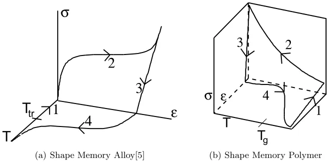
Shape memory alloys are materials that are metallic in nature whose shape recovery processes are enthalpy driven. The typical shape recovery process (Figure 1(a)) [5] begins at a temperature above the transition temperature, Ttr. In this state, the austenite cellular configuration is dominant and stable. The alloy is then cooled below

Ttr. During the cooling process, the austenite configuration becomes unstable (this happens around Ttr) and

the cellular configuration transitions to twinned martensite.

Once the alloy is belowTtr, it is deformed with an applied stress (or strain). This applied deformation causes

a strain (or stress) on the alloy which grows linearly until a critical stress is reached at which point the twinned martensite transitions to the detwinned martensite cell configuration. After the transition to the detwinned state, the applied deformation is released but a residual strain remains because of the detwinned martensite cellular configuration. In the final step of the shape recovery process, the alloy is heated above Ttr at which

point the martensite configuration returns to the stable austenite configuration. a

s

e

T

T

1

2

3

4

(a) Shape Memory Alloy[5]

s e

T

g

1

2

3

4

T

(b) Shape Memory Polymer

Figure 1. Thermomechanical cycle of (a) shape memory alloys and (b) shape memory polymers.

1.2 SMP shape recovery process

Shape memory polymers (SMPs) are materials that are rubbery in nature composed of long, intertwined polymer chains and whose shape recovery processes are entropy driven. Under tension, the polymer chains stretch to accommodate the deformation. Because of the stretching, the number of possible configurations a chain can take and, as such, the configurational entropy is decreased. The tension in the chain is not cause by a change in energy, but rather a change in entropy.

The typical shape recovery process for small deformations (see Figure 1(b)) begins at a temperature above the glass transition temperature,Tg.At this temperature, the polymer is in a rubbery elastic (active) state. The

polymer is then deformed with an applied stress (or strain) which creates a strain (or stress) in the polymer.

Once the polymer is deformed, it is cooled below Tg at which point the active polymer becomes inelastic

(frozen or glassy). The applied deformation is removed, however the polymer remains in its deformed state because the deformation becomes “locked” in place belowTg. The resulting deformation creates a residual strain

which remains present until the shape recover process is completed when the polymer is heated aboveTg.

It is important to note that polymers at low deformation levels (compared to what they are capable of sustaining) exhibit a fully recoverable linear elastic behavior. If an undeformed polymer is cooled belowTg and

then deformed, once the external forces are removed it will return to its previous undeformed state.

1.3 Comparison of SMPs with SMAs

Whereas the shape recovery process in shape memory alloys is a result of different cellular configurations in which they can exist, the shape recovery process in shape memory polymers is governed by the transition from an active state to a frozen state (and back again). Figure (2) illustrates a representative volume which contains both frozen and active parts of the polymer.

The microstructure of a shape memory polymer can vary based on how the polymer is synthesized including entanglement of polymer chains, cross-linking, crystallization and the formation of domain structures. This polymer interaction gives each polymer volume unique properties.

Shape memory alloys are known to have large recovery pressures (as much as 500 MPa). They are also able to dissipate energy greatly when going through the shape recovery process. However, SMAs are only able to recover from deformations up to 10%, above which plastic deformation with unrecoverable shape change can occur. Also, they are subject to internal heating and metal fatigue, both of which degrade the reliability of SMAs.

On the other hand, SMPs can recover from deformations well over 100% and can go through a high number of repetitions without any significant material degradation. BelowTg, SMPs do sustain plastic deformations,

Figure 2. Frozen and active portions of a polymer. [3]

280 300 320 340

0 0.1 0.2 0.3 0.4 0.5 0.6 0.7

Temp (T)

Tan delta

Cooling Heating

Figure 3. Tan delta curve for polymer. [4]

Tg.[1] The primary disadvantage of SMPs is that the recovery pressure is several orders of magnitude below that

of SMAs (around 1-3 MPa) when transitioned through a thermomechanical cycle.

2. EXPERIMENTAL PROCEDURE

All experiments and data collection were performed by Y.+ Liu et.+ al.+ [4] where a more detailed account of experiments and procedures can be found.

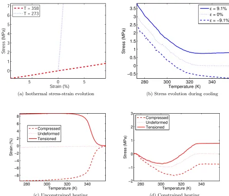
Using a commercial thermoset epoxy system intended for deployable space structure applications, thermome-chanical experiments were conducted with dog-bone shaped specimens. The first experiment was a three-point flexure test to determine the storage modulus, loss modulus, and ultimately tan delta (ratio of loss modulus to storage modulus). All polymers show similar response as a function of temperature, where the peak of the tan delta curve occurs at the glass transition temperature. Figure (3) shows the tan delta curve for the polymer in these experiments and shows a peak atT≈343K.

The bulk modulus for the polymer, in both the glassy and active states, was found by a simple ten-sion/compression test at a temperature well belowTg (T = 273K) and at a temperature aboveTg (T = 358K),

Stress evolution occurs for a constant strain condition when the temperature varies. This is most notably due to thermal strain attempting to contract the sample. Figure (4(b)) illustrates the cyclic stress evolution during a cooling-heating cycle for three different pre-deformed states: tensioned, compressed, and undeformed. This experiment is analogous to curve 2 of the SMP thermomechanical cycle depicted in Figure (1(b)).

After the stress evolution during the cooling process for a constant strain, the applied strain can be removed at which point the polymer will “spring back” to a fixed strain. This is depicted in Figure (1(b)) at the junction point between curves 3 and 4. This fixed strain is essentially how much deformation has been “locked” in the cooling process and is typically smaller in magnitude than the applied deformation.

At this point, there are two options from this stress-free point: unconstrained heating (zero stress throughout), or constrained heating (constant strain throughout). Unconstrained heating is when no strain is applied to the polymer during heating and it is allowed to return to its original shape by allowing the internal stresses to reach an equilibrium throughout the process. Figure (4(c)) depicts this process as a temperature-strain relationship. In contrast, constrained heating is when the deformed polymer is kept at a constant strain through the heating process generating internal stress. Figure (4(d)) depicts this process as a temperature-stress relationship.

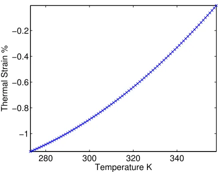
Also necessary for model implementation is the thermal expansion coefficients. During the heating and cooling process, the polymer volume contracts and expands due to thermal strain. Figure (5) shows the unconstrained uniaxial thermal strain. The thermal expansion coefficient (defined by the slope of the thermal strain) is obtained in both the frozen and active regimes to beαf = 1.2×10−4 andα_a= 1.8_×10−4.

3. CHARACTERIZATION OF STRAIN IN SMPS

Polymers undergo a transition from high-stiffness to low-stiffness and back through heating and cooling processes respectively. The temperature at which this transition takes place is known as the glass transition temperature, Tg, and characterization of the polymer on both sides of this transition point is necessary due to the marked

differences.

3.1 Components of strain

The description of strain follows the work done in ??. We begin with a shape memory polymer that has total volumeV (which may be a function of temperature). As the whole volume undergoes a temperature change, the volume will contain both a frozen and active portion. These volume fractions are denoted as

φf =

Vf rz

V , φa = Vact

V ,

whereφf+φa= 1.Under sufficiently slow heating and cooling processes, as well as sufficiently slow strain rates,

it can be assumed that the phase fractions are strictly dependent on temperature.

Because of the different phases present in the volume, the total strain can be characterized as the sum of the strain in each phase fraction. Therefore, we write

ε=φfεf+ (1−φf)εa. (1)

In the frozen phase, the entropic portion of the pre-deformation is assumed to be completely locked and stored during cooling. Due to the localized freezing process, the entropic frozen strainεe

f, can be anisotropic inside the

ever-growing frozen phase and should be considered as a function of the position vector,x. [4] Deformation in the frozen phase comes from the sum total of three parts:

• the average of the frozen entropic strain,

• the internal energetic strainεif, and

5 0 5 0

1 2 3 4 5 6 7

Strain (%)

Stress (MPa)

T = 358 T = 273

(a) Isothermal stress-strain evolution

280 300 320 340

−0.5 0 0.5 1 1.5 2 2.5 3 3.5

Temperature (K)

Stress (MPa)

ε = 9.1%

ε = 0%

ε = −9.1%

(b) Stress evolution during cooling

280 300 320 340

−8 −6 −4 −2 0 2 4 6 8

Temperature (K)

Strain (%)

Compressed Undeformed Tensioned

(c) Unconstrained heating

280 300 320 340

−2 −1 0 1 2 3

Temperature (K)

Stress (MPa)

Compressed Undeformed Tensioned

(d) Constrained heating

280 300 320 340 −1 −0.8 −0.6 −0.4 −0.2 Temperature K

Thermal Strain %

Figure 5. Thermal strain of polymer.

Deformation in the active phase come from the external stress-induced entropic strainεe

a and the thermal strain

εT

a.Therefore, equation (1) becomes

ε=

"

1 V

Z Vf rz

0

εefdv

#

+

φfεif+ (1−φf)εea

+

φfεTf + (1−φf)εTa

. (2)

The first term is considered to be thestored strain εs, and can be rewritten as

εs=

1 V

Z Vf rz

0

εef(x)dv=

Z φf

0

εef(x)dφ (3)

where φ= v/V. The second term is considered the mechanical (elastic) strain εm and, under the assumption

that the material behaves in a linear elastic manner in both the active and frozen phases, εi f and ε

e

a can be

related to the stress via Hooke’s law. Thus,εi

f =Siσ andεea=Seσ where Si andSeare the elastic compliance

corresponding to the internal energetic and entropic deformation respectively. Therefore the mechanical strain can be written as

εm= [φfSi+ (1−φf)Se]σ. (4)

The final term is considered to be the thermal strainεT and can be rewritten in terms of the thermal expansion

coefficientαfrom a reference temperatureT0. Therefore,

εT =

Z T

T0

[φfαf + (1−φf)αa]dθ (5)

whereαf andαa are the thermal expansion coefficients of the frozen and active phases respectively.

Equation (2) can be rewritten as

ε=εs+εm+εT (6)

=

Z φf

0

εe

f(x)dφ+ [φfSi+ (1−φf)Se]σ+

Z T

T0

[φfαf+ (1−φf)αa]dθ (7)

which yields the constitutive relationship

σ=E ε−

Z φf

0

εef(x)dφ−

Z T

T0

[φfαf+ (1−φf)αa]dθ

!

where

E= 1

φfSi+ (1−φf)Se

(8b)

is the Young’s modulus for the overall volume of the polymer.

3.2 Constitutive equations

To fully define the necessary constitutive equations for this model, we begin with stress as a function of strain, temperature, frozen fraction, and frozen entropic strain:

σ(ε, T, φf, εef) =E(ε−εs−εT) (9a)

where

E= _φ 1 f

Ei +

1₋φf

Ee

(9b)

is the Young’s modulus for the overall volume of the polymer.

We recall equation (3) which statesεs=

Rφf

0 ε

e

fdφand by the fundamental theorem of calculus, this implies

that

dεs

dT =ε

e f

dφf

dT . (10)

However, under the assumption that the entropic portion of the pre-deformation is completely frozen and stored during cooling, we can assume that εe

f =ε e

a =Seσ. Therefore equation (10) can be rewritten as the first order

differential equation

dεs

dT =Seσ dφf

dT =SeE(ε−εs−εT) dφf

dT (11a)

εe

f(Th) = 0 (11b)

where This some temperature sufficiently aboveTg.

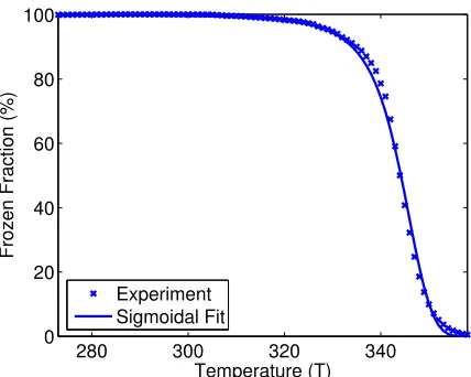
The frozen fractionφf is chosen to be a sigmoidal [4] of the form

φf = 1−_{1 +c} 1

f(Th−T)n. (12)

In order to find the unknowns n and cf, is fit to the curve defined by the modified recovery strain (tensioned

free-recovery curve in Figure 4(c) divided by the pre-deformation strain). With this curve fitting (shown in Figure 6), the parameters identified arecf = 2.76×10−5andn= 4.

The inelastic modulus is taken to be a constant as once the polymer chains become locked in a glassy state, it will not evolve with temperature. Experimentally, it is found thatEi= 813.The elastic modulusEeis considered

a linear function of absolute temperature andEe= 3N kT whereN is the cross-link density andkis Boltzmann’s

constant. N is experimentally found to be approximately 1.6379×10−21.

Equation (5), along with the experimentally found thermal expansion coefficients, can be rewritten in terms of a differential equation (to admit implicit definitions of φf in the future) by

∂εT

∂T = 0.00012φf(T) + 0.00018(1−φf(T)), εT(T0) =ε

0

T. (13)

These constitutive equations closely follows the work in [4]. Currently, differences are in the determination in thermal coefficients and thermal strain, however work is ongoing to better define the frozen fraction as a function of temperature, rate of change in temperature, and distance away from the glass transition temperature, Tg.

While fitting functions to data will increase computational speed, determining φf based on experimental data

280 300 320 340 0

20 40 60 80 100

Temperature (T)

Frozen Fraction (%)

Experiment Sigmoidal Fit

Figure 6. Comparison of sigmoidal in (12) with modified recovery strain

4. MODEL VALIDATION

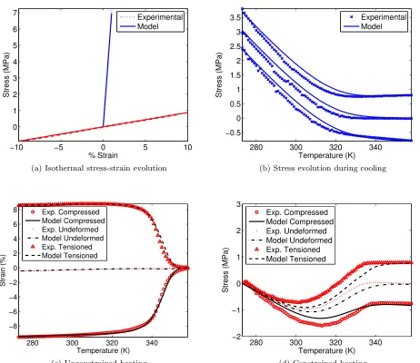
Figure (7) illustrates the models prediction of the experiments outlined in section 2. Figure (7(a)) is the isother-mal experiment with model prediction. Because the temperature remains constant, the model simplifies to the linear relation

σ=Eε (14)

since εs and εT are both temperature dependent. The high accuracy is apparent since the bulk modulus E is

found experimentally atT = 273 andT = 358.

Figure 7(c) illustrates the model’s prediction of the constrained heating data. Again, the apparent accuracy is due the determination of the frozen fraction in equation (12) is found by fitting the sigmoidal to the tensioned data.

Although figures (7(b)) and (7(d)) do not appear to be numerically accurate, the model accurately predicts the overall behavior of the different experiments and the proposed constitutive equations appear to be promising.

5. CONCLUSIONS

A phenomenological model for the shape recovery process of shape memory polymers is proposed. The prediction of the thermomechanical cycle of SMPs while remaining in the linear elastic regime with small deformations (<10%) will be instrumental as a building block for the future research of system responses and development of models involving large deformations (>>10%).

ACKNOWLEDGMENTS

The research of R.D.S. was supported in part through the NSF Grant DMS-0636590, EMSW21-RTG program. The research or R.C.S. was supported in part by the Air Force Office of Scientific Research through the grant AFOSR-FA9550-04-1-0203.

REFERENCES

[1] Christian G’Sell. Dislocations in glassy polymers do they exist? are they useful? Materials Science and Engineering, 2001.

[2] Andreas Lendlein and Robert Langer. Biodegradable, elastic shape-memory polymers for potential biomedical applications. Amer. Assoc. Adv. Sci., 2002.

−10 −5 0 5 10 0

1 2 3 4 5 6 7

% Strain

Stress (MPa)

Experimental Model

(a) Isothermal stress-strain evolution

280 300 320 340

−0.5 0 0.5 1 1.5 2 2.5 3 3.5

Temperature (K)

Stress (MPa)

Experimental Model

(b) Stress evolution during cooling

280 300 320 340

−8 −6 −4 −2 0 2 4 6 8

Temperature (K)

Strain (%)

Exp. Compressed Model Compressed Exp. Undeformed Model Undeformed Exp. Tensioned Model Tensioned

(c) Unconstrained heating

280 300 320 340

−2 −1 0 1 2 3

Temperature (K)

Stress (MPa)

Exp. Compressed Model Compressed Exp. Undeformed Model Undeformed Exp. Tensioned Model Tensioned

(d) Constrained heating

[4] Yiping Liu, Ken Gall, Martin L. Dunn, Alan R. Greenberg, and Julie Diani. Thermomechanics of shape memory polymers: Uniaxial experiments and constitutive modeling. International Journal of Plasticity, 22:279–313, 2006.

[5] Ralph C. Smith. Smart Material Systems: Model Development. SIAM Frontiers in Applied Mathematics, 2005.