Karen E. Daniels, Jonathan E. Kollmer, and James G. Puckett
Citation: Review of Scientific Instruments 88, 051808 (2017); doi: 10.1063/1.4983049
View online: http://dx.doi.org/10.1063/1.4983049
View Table of Contents: http://aip.scitation.org/toc/rsi/88/5
Photoelastic force measurements in granular materials
Karen E. Daniels,1Jonathan E. Kollmer,1and James G. Puckett2
1Department of Physics, North Carolina State University, Raleigh, North Carolina 27695, USA 2Department of Physics, Gettysburg College, Gettysburg, Pennsylvania 17325, USA
(Received 11 December 2016; accepted 26 March 2017; published online 26 May 2017)
Photoelastic techniques are used to make both qualitative and quantitative measurements of the forces within idealized granular materials. The method is based on placing a birefringent granular material between a pair of polarizing filters, so that each region of the material rotates the polarization of light according to the amount of local stress. In this review paper, we summarize the past work using the tech-nique, describe the optics underlying the techtech-nique, and illustrate how it can be used to quantitatively determine the vector contact forces between particles in a 2D granular system. We provide a description of software resources available to perform this task, as well as key techniques and resources for building an experimental apparatus.Published by AIP Publishing.[http://dx.doi.org/10.1063/1.4983049]
I. INTRODUCTION
Photoelasticity has long been used by engineers to quan-tify the internal stresses within solid bodies.1 The technique is based on the understanding, dating to Maxwell,2 that light can be polarized (the electric and magnetic fields have a well-defined orientation) and its speed depends on the medium’s index of refraction. Many crystalline materials are birefrin-gent: their crystalline axes specify a fast and slow direction for the propagation of light.
Non-crystalline materials such as polymers and glasses can nonetheless bephotoelastic, with the degree of birefrin-gence at each point in the material depending on the local stress. When a photoelastic material is placed between two polarizers and subjected to stress, each region of the mate-rial rotates the polarization of light according to the amount of local stress and the stress-optic coefficient of the material. This creates a visual pattern of alternating bright and dark fringes within the material, and this pattern depends in a detailed way on the orientation of the polarizers, the shape of the material, and how it is stressed.
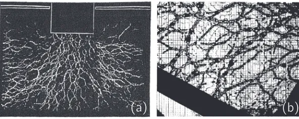
Before the creation of finite-element computing meth-ods, photoelastic analysis was a key technique for predicting regions of high compressive or tensile stress during the design of manufactured parts. As such, it has been an important part of engineering practice in both its qualitative and quantitative forms.3–6It was therefore inevitable that photoelastic methods eventually be applied to the study of idealized conceptions of granular materials, as was first done by Wakabayashi using epoxy tracer particles in 1950s,7 followed by Dantu (using ordered/disordered arrays of glass cylinders8) and later by Drescher and de Josselin de Jong9 (in polymer disks) and Liu et al.10 (in glass spheres). The network-like structures visible in Figs. 1 and 2 have come to be known as force chains.
These pioneering experiments played a key role in the physics community’s realization that heterogeneous force transmission identifiable at the particle scale is of great impor-tance for understanding the mechanics of granular materi-als.10,11 A series of papers by Behringer and co-workers
established the photoelastic method as the key technique for making quantitative advances.12–14 In the past two decades, many different experimental teams have used pho-toelastic force visualization to quantify myriad phenomena. For example, it has been possible to reveal the particle-scale anisotropy of the contact force networks,15 identify interparticle contacts,16,17measure fabric and stress tensors,18 examine particle shape dependence,19 test the validity of statistical ensembles,20 identify dilatancy-softening,21 mea-sure force chain order parameters,22 evaluate the grain-scale stresses caused by growing plant roots,23,24observe the effects of fluid flow,25 follow slow dynamics under shear,13,26–28 and quantify fast dynamics.29–32 Because the photoelas-tic response is known analyphotoelas-tically for circles/ellipses, sev-eral of these studies have measured the vector contact forces at every interparticle contact within the granular material.33–35
This paper first provides a review of photoelasticity and how it can be used to create high-quality images of stress within the granular material (SectionII). These images can be used either semi-quantitatively (Section III) or quantita-tively (SectionsIVandV), with the latter providing a method to determine the vector contact forces for each of many cir-cular particles in the system. We provide a description of software resources available to perform this task. Finally, we describe key techniques for building an experimental appara-tus (SectionVI), including resources for the purchase of key components.
II. Photoelasticity
This section provides a brief overview of polarized light and photoelasticity, to aid the reader in building a qualita-tive understanding of the method. A standard optics text-book (such as Hecht36) can provide quantitative details about polarized light, and the classic two-volume monograph by Frocht1 provides a comprehensive treatment of photoelastic-ity as a method. Several recent book chapters also provide an introduction to the method’s use in the context of granular materials.35,37
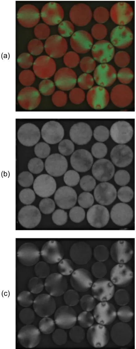
FIG. 1. Historical examples of force chains in (a) glass cylinders viewed via darkfield photoelasticity. From Dantu, Proceedings of the Fourth International Con-ference on Soil Mechanics and Foundation Engineer-ing, London. Copyright 1957. Reprinted with permission from Butterworth’s Scientific Publications.8(b) Polymer
disks viewed via brightfield photoelasticity. Reprinted with permission from Drescher and de Josselin de Jong, J. Mech. Phys. Solids20, 337 (1972). Copyright 1972 Elsevier.9
A. Polarized light
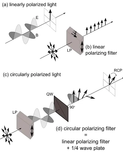
Electromagnetic waves travel in a direction co-perpendicular to the sinusoidal electric and magnetic fields of which they are comprised (see Fig.2(a)). Linearly polar-ized light consists of waves that all have the same orientation of their electric fields. Two common ways to generate lin-early polarized light are reflection from a metallic surface and transmission through a polarizing filter (also known by a brand name, PolaroidTM). These filters consist of a thin sheet of iodine-impregnated polyvinyl alcohol, with polymer chains preferentially aligned along one axis. The mechanism through which they polarize the light is that the iodine provides conduction electrons which polarize along the polymer chains and thereby cancel the electric field of the incident light polar-ized in the parallel direction but not in the perpendicular direction. Typically efficiencies are to absorb>95% of light in the parallel direction and transmit <40% of light in the perpendicular direction.38
Circularly polarized light consists of electric and mag-netic fields that remain mutually perpendicular but rotate with constant magnitude with left-handed (counter-clockwise) or right-handed chirality (clockwise) with respect to the direc-tion of propagadirec-tion. To create circularly polarized light, light is first linearly polarized and then passes through a quarter wave plate that advances the phase of one polarization with respect to the other. A quarter wave plate is a birefringent material of chosen orientation (fast/slow axes) and thickness
FIG. 2. A modern example of darkfield photoelasticity; particles that appear brighter and with more fringes are those experiencing large forces. Within each bright grain, the number of alternating bands of light/dark fringes increases with average stress on the particle, an effect shown in more detail in Figs.7
and8.
matched to the wavelength of interest. The orientation of the fast axis at±45◦ (see Fig.2) with respect to the linear ization determines whether the output is left-circularly polar-ized (LCP) or right-circularly polarpolar-ized (RCP). Typically, the two optical elements are purchased as a single, fused unit. Note that, unlike linear polarizers, a circular polarizer can be arbitrarily rotated by any angle around the transmission axis with no effect on the filtered light but cannot be flipped over.
B. Polariscopes
The basic principle of a darkfield polariscope is to place a photoelastic sample between a polarizer and an analyzer of the opposite polarization (e.g., vertical and horizontal linear polarizers or LCP and RCP circular polarizers), viewed in transmission. Sample configurations are shown in Fig.4. Note that care must be taken during the installation of circular polar-izers, to ensure that the polarizer and analyzer are both placed with their quarter-wave plates facing the sample.
In each case, initially unpolarized light becomes polarized after passing through the polarizer. As the light passes through the sample, the amount of birefringence at each point depends on the local stress state (photoelasticity). This birefringence causes the light to rotate its polarization as it passes through the sample, and when it exits the sample the polarization has been rotated by a total ofθdegrees. The light now passes through a final polarizer called the analyzer. The final intensity of light depends on the local stress in the birefringent sample as well as the orientation of the analyzer. In a stressed sample, this leads to an image of light and dark fringes (see Fig.3).
While both linear and circular polariscopes are possible, there is a practical difficulty with linear polariscopes that limits their utility: In a linear polariscope, there are two possible reasons for fringes to appear: (1) the photoelastic response of the sample rotates the polarization to match/mismatch the analyzer; and (2) if the principal stress of the sample happens to be aligned with the polarizers, it will not be affected by the photoelastic response of the material. Therefore, for linear polariscopes, the fringe pattern depends on both the relative angles between the polarizer (fixed) and the principal stress (changes at different locations and times during experiment). For this reason, quantitative work with polariscopes should always be conducted with circularly polarized light, which provides azimuthal symmetry.
FIG. 3. (a) Linearly polarized light has its electric (E) and magnetic (B) fields oscillating in-phase and mutually perpendicular to the direction of propaga-tion. The axis of the electric field specifies the direction of polarizapropaga-tion. (b) Linearly, vertically, polarized light is created by the transmission of unpolar-ized light through a linear polarizing filter which attenuates the electric field components in the horizontal direction. ((c) and (d)) Circularly polarized light has its electric and magnetic fields oscillating 90◦out of phase and mutually perpendicular to the direction of propagation. The chirality of the rotation of the electric field component specifies the direction of polarization. Circularly polarized light is created by the transmission of unpolarized light through a linear polarizing filter which attenuates the electric field components in the horizontal direction, followed by a quarter-wave plate which creates the 90◦ phase shift between the electric and magnetic fields. The fast/slow axes of the quarter-wave plate are rotated by 45◦degrees with respect to the linear polarizer.
ambiguity in the phase. Various groups have proposed vari-ous methods to unwrap the phase map of the resulting image to extract the stress in the sample. However, many images of the sample are needed with different wavelengths of light39 and different analyzer orientations.40 These methods must resolve both isochromatics (associated with the magnitude of local stress) and the isoclinics (the angle of stress). In investigations of granular materials, we are solely interested in the contact forces of each sample rather than the local stress state itself. Therefore, it is sufficient for contact-force measurements to use an analyzer which has been arbitrarily rotated about its azimuthal axis (with respect to the polar-izer); this results in an image of the isochromatics only. Throughout the remainder of the text, we assume images are acquired using the circular polarizers set up as shown in Fig.4.
Generally speaking, the samples in Figs.1and2illustrate that particles with more force are brighter (darker) against a dark (bright) background because the light that passed through them had its polarization rotated. Often, this contrasting effect is sufficient to identify general features of stress-transmission within a granular sample. Methods for quantifying these fea-tures are described in Section III. Importantly, there is a quantitative, one-to-one mapping between the stress field in
FIG. 4. Schematic diagrams of sample (a) linear and (b) circular darkfield transmission polariscopes. For brightfield polariscopes, the polarizer and ana-lyzer would match (e.g., two RCP polarizers, both with their quarter-wave (QW) plates facing inwards and the linear polarizers (LPs) facing outwards).
the sample and the resulting pattern of fringes.1 Therefore, it is possible to solve the inverse problem and use polariscope images to determine the vector contact forces on each parti-cle in the sample. Quantitative methods for performing this inversion are detailed in SectionsIVandV.
III. SEMI-QUANTITATIVE MEASUREMENTS
Originally, images of the type shown in Figs.1and2were used for semi-quantitative investigations, without the knowl-edge of the vector contact forces between the particles. Even in modern experiments, there is much that can be learned from comparing the spatial patterns of the force chains. For exam-ple, images of the force chains can reveal history dependence via spatial correlations,41,42 the ensemble-averaged response to point forces,43and the principal axis of the response.44By subtracting images taken before/after an event, it is possible to examine spatial patterns of failure26,45 and the speed of sound.31
To quantify how the number of dark/light fringes increases with the stress on each particle, Behringer and co-workers11,13,14,46 calculated the squared local gradient, averaged over all pixels in an image
hG2i=X
i,j f
(Ii+1,j−Ii−1,j)2+ (Ii,j+1−Ii,j−1)2
+1
2(Ii+1,j+1−Ii−1,j−1)
2+1
2(Ii+1,j−1−Ii−1,j+1)
2g
. (1)
FIG. 5. (a) Sample darkfield image illustrating the gradient-squared (G2) technique given by Eq.(1). (b)
SampleG2calibration data. Reprinted with permission
from Howellet al., Phys. Rev. Lett.82, 5241 (1999). Copyright 1999 American Physical Society.11
TheG2method has several important advantages over the
photoelastic inverse methods to be described in SectionV. First, it works on low-resolution images (10 pixels/particle is enough) as long as there is sufficient intensity contrast. Second, image processing times are very fast: at the time of writing, it takes 0.05 s to calculate the pressure within a 1 megapixel image on a single processor. Finally, there are no parameters in Eq. (1). To translateG2 into pressure, only a single calibration experiment needs to be done under the same lighting conditions as the experiment, in order to properly account for the image intensity and contrast. For these rea-sons, theG2method has remained popular, even as the speed
and accuracy of vector contact force measurement codes have improved.
IV. PHOTOELASTIC THEORY
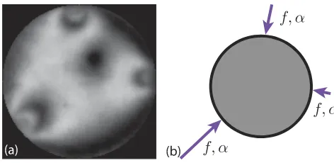
As illustrated in Fig. 6, a set of z contact forces on a disk determines the pattern of photoelastic fringes. Because the analytical solutions for the stress created by point contact forces on a disk are known,1 it is possible to determine the intensity fieldI(x,y) from the set ofzvector forces. In ana-lyzing images from experiments (to be shown in SectionV), we will need to do the inverse: for a knownI(x,y) recorded by a camera, determine the vector contact forces which cre-ated that image. In this section, we present the theory required to determine the mapping from~f→I and calibrate the mea-surements so that they can be used for the inverse problem in Sec.V.
FIG. 6. (a) A image of the isochromatic stress on a disk withz= 3 contacts, and (b) a schematic of possible contact forces acting on the disk, with force magnitudef and impact angleα.
A. Solution for diametric loading
The special case of diametric loading provides both an instructive example for understanding quantitative photoelas-ticity and the means of calibration necessary for any quan-titative experiment. As illustrated in Fig. 7, the number of dark/light fringes increases with the diametric load of mag-nitudef (equal and opposite forces along the diameter of the disk). We can understand this behavior starting from the known solutions for the stress tensor at the center of the disk,1,50
σxx=
2f
2πRh, (2)
σyy=−
6f
2πRh, (3)
σxy=0. (4)
The intensity of the fringe pattern at any point is given by
I(x,y)=I0sin2
π(σ1−σ2)hC(λ)
λ , (5)
where (σ1−σ2) is the difference in the principal stress at the
point (x,y),h is the material thickness,λis the wavelength of light, andC is the stress-optic coefficient (aλ-dependent material property).
The spatial variations inI, visible in Fig.8, are present because σ1 −σ2 is spatially varying. We will consider the
simpler case of monochromatic light, so that Fσ=λ/Ch
FIG. 7. Comparison of observed image (bottom) and pseudo-image calcu-lated from Eq.(6)(top) for a set of eight diametrically compressed disk with
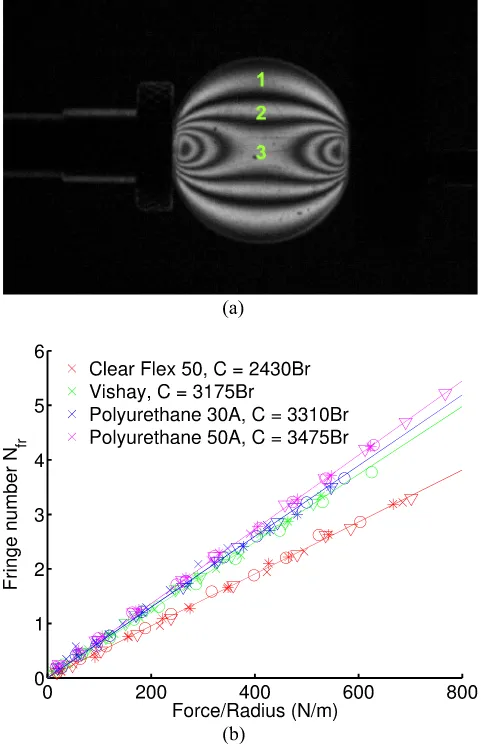
FIG. 8. (a) Sample fringe counting for the disk withNfr= 3. (b) Calibration
ofFσ for 4 different photoelastic materials. The units of the stress-optic coefficient are in Brewsters: 1 Br = 1012m2/N.
(the stress-optic coefficient) is a constant. In the case of isochromatic fringes, Eq.(5)reduces to
I(x,y)=I0sin2
π(σ1−σ2)
Fσ . (6)
Using Eq. (4), we have σyy=−3σxx, where the
off-diagonal componentsσxyandσyxare zero and the shear stress
is zero at the center of the disc. The difference in the principal stress is the difference in the eigenvalues, which then is given byσ1−σ2=|σxx−σyy|. Then, at the center of the disc, the
number of fringesNfris given by
λ
hC =
σ1−σ2 Nfr =
4f πRNfrh
. (7)
For an unstressed disk, σ1=σ2=0 everywhere in the
disk, the difference in the phase is zero and thus the isochro-matic image is dark. The first bright fringe occurs when the difference in the principal stress isσ1−σ2=Fσ/2. The bright
and dark fringes on the disk arise from the periodic function (sin2x) in the phase retardation. As shown in Fig.7, the total number of fringes increases as the sin function cycles through an increasing number of bright and dark fringes for increasing values ofσ1−σ2.
Thus,Fσcan be empirically determined by diametrically compressing the disk by a known force and recording the fringe number as follows. For diametric loading, the fringe number is defined as the number of fringes counted between the edge of the disk and the center of the disk, as shown in Fig.8(a). The fringe number at the boundary is zero. Moving toward the center, each bright/dark band increments the fringe number by 0.5. In order to measureC(the material parameter), a typical experiment proceeds by placing a disk of known radius and thickness into a load cell and illuminating it with monochro-matic, polarized light. As the diametric load on the particle is slowly increased, a measurement is taken each time a new fringe appears (Nfr increases). A scatter plot of the diametric
force and number of fringes allows for a fit to the left and right sides of Eq. (7). Since all other parameters are known, this provides a measurement ofCfor that particular material, as shown in Fig.8(b). Most of the commonly used materials (see SectionVI A) haveC≈3000 Br.
B. Solution for arbitrary contacts
Ultimately, we will determine all contact forces acting on a particle based on the pattern of isochromatic fringes recorded in images of photoelastic disks. This goal is illustrated for a single particle in Fig.6. To achieve this will require a formula for the solutionI(x, y), as a function of an arbitrary set ofz vec-tor contact forces, acting at arbitrary contact locations around the perimeter of a disk. In this section, we derive the solution to the stress fieldσ(x,y) inside an elastic disk in mechanical equilibrium withzpoint forces on the boundary, along with a short review of the necessary theory of elasticity. The solution presented here largely follows the work by Refs.1,50, and51. For any linear elastic solid with boundary forces, there are three basic assumptions: (a) the condition of equilibrium (force and torque balance); (b) a constitutive relation (here, linear stress-strain); (c) Saint-Venant’s condition of compatibility (no gaps or overlaps). In two dimensions and in the absence of body forces, the condition of equilibrium for a static solid is given by
∂σxx ∂x +
∂σxy ∂y = 0, ∂σyy
∂y + ∂σxy
∂x = 0.
(8)
Equivalently, ∇ · σ=0. The second assumption is a linear relation between the strain and stress tensors,
σ=k. (9)
The third assumption is Saint-Venant’s condition: the solid deforms continuously leaving no gaps and creating no over-laps.52 For plane strain in the absence of body forces, the compatibility of infinitesimal strains is given by
∂2 ∂x2 +
∂2 ∂y2
!
(σxx+σyy)=0. (10)
The solution to Eq.(10)in two dimensions is solved using Airy stress functions,ϕ, where the components of the stress tensor are derivatives ofϕ,
σxx= ∂2ϕ
∂y2, σyy= ∂2ϕ
∂x2, σxy=− ∂2ϕ
Then the compatibility equation of the stress function is biharmonic
∂2 ∂x2 +
∂2 ∂y2
! ∂2ϕ
∂x2 + ∂2ϕ ∂y2
!
=0,
∇4ϕ=0. (12)
In general, the solution to Eq. (12) is guessed by using symmetries or adjusting a known solution to the boundary conditions.
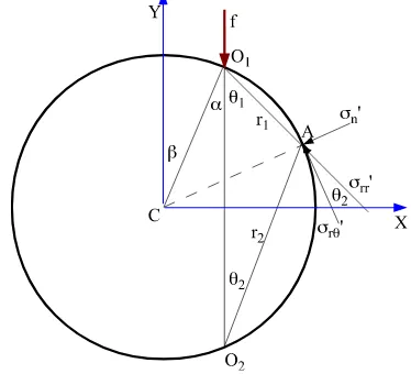
Consider a stress on a disk, as shown in Fig.9, with radius Rand thicknessh. We define the origin at pointO1where the
direction of pressure isO1O2, with anglesθ1andr1as shown
in Fig. 9. Points on the circumference of the circle have a radial stress σrr=−π2fhcosθ in the direction r1. The angle
between σrr0 and the tangent is θ2. The components of the
stress tensor are σ0
rr =σrrsin2θ2, σ0
rθ =σrrsinθ2cosθ2, σ0
θθ=0.
(13)
Substituting σrr and using θ=θ1 and r1=2Rsinθ2
every-where on the circumference, then
σ0
rr =− f
πRh[sin(θ1+θ2) + sin(θ1−θ2)] , σ0
rθ =− f
πRh[cos(θ1+θ2) + cos(θ1−θ2)]
(14)
These two tensors are the superposition of three stresses at pointAon the circumference as follows:
• normal stress:−πf
Rhsin(θ1+θ2). • tangential stress:−πf
Rhcos(θ1+θ2).
• uniform stress in the direction of r1 with normal
and tangential components: −πf
Rhsin(θ2 − θ1) and
−πf
Rhcos(θ2−θ1), respectively.
If the disk is force and torque balanced, torque balance impliesPz
ificos(θi,1+θi,2)=0, and the sum of the uniform
tension must also be zero. Therefore, the remaining term is the sum of the normal tensions at the boundaryPz
i fi
πRhsin(θi,1
+θi,2) along the circumference, which is simplified using the
inscribed angle theoremθ1+θ2=π2 ±αand the identity sin(π2
FIG. 9. A disk with a force,f, at pointO1at an impact angle (direction)α.
±α)=cos(±α)=cosα. To ensure that the boundary of the disk is stress free, a uniform tension of magnitude πfRhcosα is added to the radial stress distribution. The solution forz concentrated forces on a disk whereθiis the angle betweenfi
andriandαas shown in Fig.9is
σrr= z
X
i=1
−2fi πRh
cosθi ri +
z
X
i=1 fi
πRhcosαi. (15)
All other components ofσare zero.
The solution is inz-polar coordinates. To write the solution in a single coordinate system, we use a Cartesian coordinate system with the origin at the center of the disk. Letβbe the angle between the positiveY-axis and the line segmentCO1,
as shown in Fig.9. We computeσrr as in Eq.(15)and
trans-forming coordinate systems with a rotation byθi=−(βi+αi)
as
σ= z
X
i=1
T(θi)σi,rr T−1(θi), (16)
whereT(θi) is the rotation matrix.
The eigenvalues ofσare
σ1,2=
1
2 (σxx−σyy)± q
(σxx−σyy)2+ 4σ2xy
!
, (17)
where the subscripts 1 and 2 correspond to the + andsigns, respectively.
We have presented the solution toz-forces on a disk and given a calibration ofFσ for the photoelastic disk. SectionV
details the numerical methods involved in taking this solution and finding the contact forces in an array of disks.
V. AUTOMATED INVERSION
The ultimate goal of the force-inversion process is to start from images such as Fig.10, find all of the particles, and determine the vector contact forces between them using the theoretical framework described in SectionIV. While the equations for the image intensity due to a known set of par-ticle positions and contact forces are known analytically, the inverse of the problem is not. Several research groups15,20,28,35 have created computational solutions to this inverse problem, including in C++53 and MATLAB,54 a technique pioneered more than a decade ago33by Majmudar.
Here, we describe our most recent implementation, PEGS, inspired by the earlier work of Majmudar33 and Puckett.34 PEGS is written for the MATLAB platform and is avail-able for download and development on the GitHub open source software platform.54 It makes use of Matlab’s built-in parallelization toolbox, makbuilt-ing it suitable for runnbuilt-ing on high-performance computers to reduce computational time.
In general, it is necessary to have two images for each experimental configuration: one taken in unpolarized light for detecting particle locations, and one taken in polarized light for measuring the forces on those particles.16Several possible ways to do this are discussed in SectionVI D.
FIG. 10. (a) Sample RGB image color recorded from the experiment, decom-posed into (b) the red channel, taken in unpolarized light to show the particle positions, and (c) the green channel, taken in circularly polarized light to show the internal forces. The experimental setup is a reflection polariscope similar to what is shown in Fig.16.
from a setup illuminated by two monochromatic light sources: red unpolarized light and green circularly polarized light (see Fig.16). This configuration allows the camera to automati-cally collect the two necessary images within a single color frame.
The PEGS inversion process comprises three programs. Thepre-processorprogram detects particles, identifies neigh-bors, and validates which of those neighbors are contacts. This program operates on both the polarized and unpolar-ized images. The positions of the particles and contacts are then used by thefringe-inverterprogram, which performs the image-inversion process by which the photoelastic fringe pat-terns from a circular polariscope are used to determine all vector contact forces. This process operates on polarized-light images only. Finally, thepost-processor program contains a suite of tools for error-correction and visualization. This pro-vides a means to check the output for quality and then use this feedback to adjust the program’s parameters before submitting batch jobs to analyze a full dataset.
A. Pre-processor
The first step is to obtain the locations and radii of all particles in the packing, from an image such as Fig. 10(b). From experience, we find that this needs to be done with an accuracy of.0.05d in order to successfully invert the fringe pattern; the quality of the fringe-inversion fits will improve sig-nificantly with an increased centroid accuracy. We have found that the MATLABimfindcircles() function provided in the Image Processing Toolbox is able to achieve the neces-sary level of precision; other Hough transforms provide similar performance. Several algorithms are available within that func-tion, and for the results shown below we used the Hough transform (see Ref.55for a review), applied separately for each particle size. The results shown in Fig.11(a)use red/blue cir-cles to mark the locations of all particir-cles with large/small radii, respectively. Many other particle-finding routines, including convolution methods, could alternatively be used. For a review, see the work of Shattuck.35
In order for the fringe-inversion process to work effi-ciently and effectively, it is important to have a high-quality list of force-bearing contacts. The initial list of candidate-contacts is created by first identifying all neighbors by a threshold distance between the centers of a pair of particles of known radii, located at~xiand~xj. A na¨ıve definition of a
con-tact would be to call two particle concon-tacts if their separation was within some tolerancedtolof the sum of their respective
radii,
|~xi−~xj|<ri+rj+dtol. (18)
However, even with sub-pixel resolution, this method is inad-equate for determining whether the contacts are force-bearing. For each disk, the number of neighborsnsatisfying Eq.(18)
is greater than or equal to the actual number of contactsz, and dtolmust be set generously to overcome uncertainty in particle
positions.
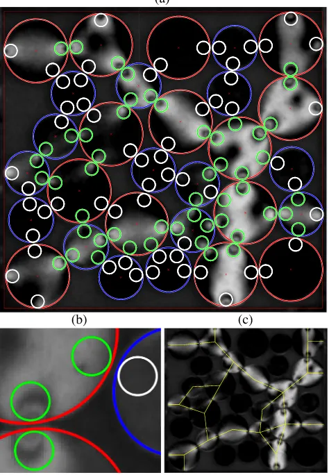
FIG. 11. ((a) and (b)) Sample image and detail showing particle-detection (large red/blue circles) and neighbor-detection (small circles). Valid contacts are identified by evaluating an area around each contact point (small circles) and comparing the photoelastic response inside the area to a threshold. While circles are below-threshold and are classified as neighbors; green circles are above-threshold and are classified as contacts. Both sides of a contact must be declared contacts; this set is shown in (c) by the yellow connectivity network.
A sample comparison is shown in Fig.11, where all of the small white and green circles indicate possible contacts, but only the green circles meet the threshold criteria for being a contact. This significantly reduces the possibility, shown in Fig.11(b), that a fringe located near the outer edge of one particle cause a false positive. This thresholding method is sensitive to having sufficient resolution and contrast. As a prac-tical measure, it is necessary to adjust the contact threshold and the size of the evaluated area around the contact point for each specific dataset. In the PEGS software,54 we pro-vide a verbose option in the program allowing the user to get a visualization of the detected contact network, as shown in Fig.11(c).
In addition, uncertainty in which contacts should be included inzcan be overcome after the fact: the force-inversion code can later determine thatfi≈0 (a null contact). This simply
increases the parameter space over which the inversion process must search, from 2z3 to 2n3. Therefore, it is better to setdtoland theG2-threshold to be generous in including likely
contacts on the list. While this will result in an increased com-putational load, the force solver is free to set the force of any contact to zero, but it is not allowed to create new contacts.
B. Fringe-inverter
Using the list of particle positions, radii, and contacts, we can iterate over all particles in the system to deter-mine which set of~f =(f,α) forces from the general solution (SectionIV B, Refs.1,50, and51) would produce the observed pattern of isochromatic fringes. In the text below, we use the same naming of the location of the contacts β, forcesf, and impact anglesαas used in Fig.9.
The inversion process proceeds one disk at a time, for which we already know the locations of thezcontacts from SectionV A. Importantly, the location of all contacts must be along the line between the two particle centers and is specified by the polar angleβ. This is satisfied by default in the algorithm described in SectionV A.
We generate an initial guess for each force magnitudef by first applying the gradient squared method from Eq.(1)
in SectionIIIto the entire disk. We then distribute this total force among thez contacts in proportion to the value ofG2 within a small area around each contact point. To make an initial guess for the angleαof each force, we select a value for which the given contact locations βand guessed values off would collectively be in force balance (see SectionV C). This is included as an optional step, since force balance will not be applicable for systems for which there is significant dynamics. Using the set ofzvalues of (f,α,β), we solve for the stress fieldσ(x,y) on a grid chosen to match the resolution of the original image. Optionally, it is possible to downscale the grid for faster computing time at a reduced resolution. Together with Eq. (6), this creates a pseudo-image Ips(f,α,β) of the
isochromatic fringes. We compare the guess to the original imageIobsby the residual function
e(f,α,β)=X
x,y
(Iobs(x,y)−Ips(x,y,f,α,β))2, (19)
where x and y are the spatial coordinates of the images. This residual function is suitable for optimizing via any stan-dard algorithm, with the values of f1...z,α1...z are varied in
order to find the minimum value for e, as was first done by Refs. 16 and 33. We have had good success using the Levenberg-Marquardt56,57 implementation contained within the MATLABlsqnonlin()function. Note, however, that this will only find alocal minimum in the (f,α) landscape and is therefore sensitive to the quality of the initial guesses. Because the stress field calculation is computationally expen-sive, we calculate theσsolutions for each grid-point in par-allel. This option, available natively in MATLAB, enables the code to run efficiently on multi-core/threaded computers or high performance computing clusters.
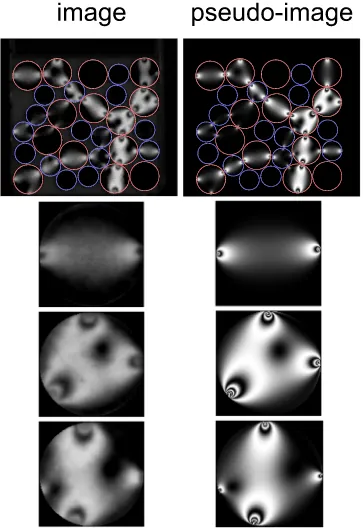
FIG. 12. Comparison of observed image (left) and pseudo-image (right) for an array of uniaxially compressed set of bidisperse disks. In the top row, the outline of the disks is shown in red (large particles) and blue (small parti-cles). In the bottom three rows, each left/right pair is an observed image (left) compared to its pseudo-image (right) for individual particles withz= 2, 3, 4 contacts, respectively.
due to the optical quality of the particles, we find that the accu-racy and efficiency of the results are improved by fitting only the innermost 0.95r of each disk rather than using all pixels up to the outermost edge.
C. Force and torque balance
For both the initial guesses (mentioned above), but also for all subsequent optimization steps, it is possible to improve the quality of the guesses by making use of force and torque bal-ances. Because these additional constraints reduce the number of unknowns in (f,α) from 2zto 2z3, we have found that this optional step greatly improves both the accuracy of the fit and the time to convergence.
Forzcontacts, the force and torque balance constraints are given by
z
X
i=1 fi,x =
z
X
i=1
fisin(αi+ βi)= 0,
z
X
i=1 fi,y=
z
X
i=1
ficos(αi+βi)= 0,
z
X
i=1 τi =
z
X
i=1
fisinαi= 0.
(20)
Forz= 2, the above equations reduce to
f2 =f1,
α2 =−α1.
(21)
By examining Fig.9,αcan be determined geometrically by the internal angles in the triangleO1O2C. The magnitude of
the contact forcef is theonlyfree parameter.
The initial test of the algorithm for minimizinge(f,α) is used on a set of diametrically compressed disks, whereIobs
is the image of the disk andfapplied is known. In Fig.8, the
result of the best fitI(f,α) is compared withIobs. Forz= 2,
initial guesses quite far from the true (f,α) will still converge; however higher fringe numbers require better initial guesses. The error in the magnitude of contact force was typically.5% and did not depend on the magnitude of the force (see Fig.13). The solution forz>2 requires a bit more work. The force and torque constraints in Eq.(20)reduce the number of free parameters by 3. To solve for these constrained parameters, one could do a coordinate transformation from (f,α) to the Cartesian (fx,fy); however this is not necessary. The solution
requires a coordinate transform of the contact locations βby rotating each contact so thatβz=0 (i.e., takingβi=βi−βz).
After, (f,α) are found, we simply rotate the coordinates back. Solving Eq.(20)forfz1,fz, andαz, we have
fz−1=
−z −2
P
i=1
fisinαi+ z−2
P
i=1
fisin (αi+ βi−βZ)
sinαz−2−sin (αz−2+βz−2−βz)
, (22)
fz= "
*
, z−1
X
i=1
fisin (αi+ βi−βz)+
-2
+*
, z−1
X
i=1
ficos (αi+ βi−βz)+
-2
#12
, (23)
αz=sin−1 * . . . .
,
−z −1
P
i=1 fisinαi
fz + / / / /
-. (24)
This will ensure a set off1...zandα1...zthat is both force and
torque balanced.
D. Post-processing
The force-inversion code provides the full set of~f=(f,α) values for each contact, and the residual scoree(Eq.(19)) for each disk. Using Newton’s third law, it is possible to quanti-tatively evaluate the reliability of the results shown in Fig.12.
FIG. 13. Scatter plot comparing the force fit for particle A→particle B and vice versa (data corresponding to particles shown in Fig.12). Solid line is
To illustrate this on the small number of example particles, Fig.13compares the force fit on one side of a contact to the (presumably identical) force fit on the other side. Ideally, all contacts would havefA→B=fB→A; therefore deviations from
this line indicate errors in the inversion process. We observe that these are of a consistent relative magnitude throughout the range of forces observed.
In addition, since each contact is subject to two indepen-dent optimizations, it is possible to flag contacts with unreli-able results. Individual values, or entire disks for which the residual scoreeis too high, can be automatically or manually replaced by the value from the opposite-contact. This feature also allows the data to be transformed so that all contacts (rather than all particles) experience force-balance, by sim-ply assigning each contact a force which is the vector average of the two independent measurements.
Visualizations such as Fig.12also provide feedback about improving the resolution and lighting. For example, the force-inversion technique is limited by resolution and contrast in Iobsand also governed by the number (and quality) of initial
guesses provided to the algorithm. In the low force limit,Iobsis
dark in the center of the disk and contacts appear as small dim spots near the perimeter. Greater image resolution and contrast can improve the accuracy of the contact forces found during optimization. Similarly, the resolution of the image also limits how well large forces are calculated, where fringes can become pixelated. Large forces (and largez) are more computationally expensive, and more/better initial guesses are required to find the correct local minimum fore(f,α).
VI. BUILDING AN EXPERIMENT
A. Making particles
Several commercially available materials are available with a uniform photoelastic response. These generally come in various stiffness and are sold in one of the two main formats: sheets, or castable liquids. Methods suitable for both formats are discussed below. Because of the expense associated with all types of particles, it is advisable to make only a dozen par-ticles in the first batch and check them between polarizers to determine whether the quality is good enough. For instance, frozen-in stresses often take the form of a bright ring around the outer edge of the particle when viewed in a polariscope. It is sometimes possible to eliminate/reduce these stresses by slow, gentle heating over a few days or weeks.
In designing the particles, several geometrical con-siderations are important. The granular materials will be most amendable to experimentation when all particles (disks/cylinders) stay in a single plane. This can be achieved by making particles which are wider than they are tall so that they do not tip over when sheared. When calculating the amount of material needed, it is helpful to cut at least 25% more particles than seem necessary; particles inevitably become lost or damaged over time, and it is difficult to later make identical particles. These are then best replaced by parti-cles made in the same batch as the others to avoid the necessity of particle-specific calibrations.
In humid climates, photoelastic particles will experience some degree of adhesion to themselves and their substrate due
to liquid bridging. One method of reducing this effect is to dust the experiment with a very small amount of baking powder, a technique pioneered by the Behringer Lab.
1. Sheet cutting
The following are common sources of sheet stock. Vishay PhotoStress Plus58 is a proprietary material with excellent uniformity. Nearly clear urethane sheets are available from var-ious industrial sources59and are a cheaper alternative. Both of these options come in sheets of various stiffness and thickness and have optical clarity and uniformity suitable for quantita-tive measurements. Sheets are available with a small amount of dye, which can improve particle-tracking. Although clear cast acrylic (PlexiglasTM) is widely available, it is generally too stiff (low Fσ) for most granular experiments. In addi-tion, it is weakly dichroic (it exhibits polarization-dependent light absorption) and is therefore not suitable for quantitative photoelastic analysis.
For any sheet material, several cutting methods are pos-sible depending on the technical capabilities of the machine shop. For circular particles, a skilled machinist can create a custom tool (see Fig.14) which acts as a spinning disk cutter to create circular particles of a specified diameter and with little waste. Alternatively, a small-sized computer-controlled mill can trace the outside of individual particles and make repeated custom (non-circular) shapes. However, the sidemill tool will waste the material in proportion to its diameter. In either case, the machinist will need to lubricate the cutter with dish soap rather than the usual machine oil, which degrades the polymer. With good lubrication, it is possible to create par-ticles with smooth edges all the way down, and no frozen-in stresses. It is also possible to use a water jet cutter to make custom shapes with little waste if care is taken to minimize the presence of a notch or flap at the starting/ending location.
Two simple cutting options, which initially seem promis-ing, are less practical than they might appear. The use of a punch is ill-advised since these leave a lip at the bottom of each particle. Unfortunately, both PhotoStress and urethane break down due to the heat of a laser cutter and release toxic gases, so these do not work. For a low-cost option, it is instead advis-able to simply use a band saw to cut strips and then particles as was done in early experiments.43
2. Casting
Both Vishay PhotoStress Plus58and urethane60,61are also available as a two-part castable liquid. Both formulations are available in a variety of stiffness and can be clear or lightly dyed. The companies provide protocols for making and releas-ing molds. Note that in order to achieve bubble-free particles, it is necessary to cure the material under vacuum. Castable liquids have allowed for the creation of particles of unusual shapes and also with magnetic inclusions.62
B. Polariscope configurations
FIG. 14. (a) Image of custom-built spinning cutters built by NCSU Instrument Shop, suitable for cutting circular disks, based on techniques developed at Duke.11,44(b) Image of a particle with frozen-in stresses. (c) Photoe-lastic particles with non-circular shapes. Reprinted with permission from Zuriguel and Mullin, Proc. R. Soc. A
464, 99 (2008). Copyright 2008 The Royal Society.19
schematically in Fig.15. If the experiment is horizontal, the upper plate could be omitted but is often included to pre-vent out-of-plane buckling of the granular layer. The pair of polarizers may be either of opposite chirality (darkfield, more common) or the same chirality (brightfield).
In principle, it does not matter whether the polarizers are inside or outside of the supporting layers. In practice, however, if the supporting layers are themselves made of a birefrin-gent material (e.g., acrylic), then the polarizers must be placed directly adjacent to the particles to avoid measuring photoe-lastic effects present in the supporting layer. The camera and lightbox will be placed on either side of this sandwich. Such a configuration has the additional difficulty, however, that the polarizers will become scratched over time.
There are several advantages in arranging the system so that the camera-side polarizer is attached directly to the camera. First, this avoids the expensive purchase of a sec-ond, large polarizing filter. Secsec-ond, easy-to-use polarizing filters are available for many commercial camera lenses (see SectionVI Cfor details).
In some cases, a transmission polariscope is undesirable when the supporting layer must be opaque. This is the case, for instance, for a porous membrane (frit) providing air-levitation as in Ref.20. To accommodate such situations, it is possible to build areflection polariscopewhich requires optical access from only one side of the granular material. This is shown schematically in Fig.16.
FIG. 15. Transmission polariscopes (a) with glass plates for which polarizers can be placed outside the system and (b) with acrylic plates for which the polarizers must be placed adjacent to the particles.
To create reflecting particles for use in a reflection polar-iscope, a simple method is to coat one side of the particles with silver spray paint (e.g., Rust-Oleum Mirror Effect, used by the Behringer Lab). These particles will reflect the incident light and simultaneously flip its polarization. Therefore, a dark-field polariscope results from configuring both the illumination source and the camera with the same chirality polarizer.
C. Polarizers
Two formats of polarizers are typically available, large sheets and camera-based filters. Care must be taken to identify which polarization is specified and to select left/right circularly polarized products as desired. For large sheets, cur-rent sources include API Optics,http://www.apioptics.com/,38 Edmund Optics,http://www.edmundoptics.com/,63and Alight
Polarizers, http://www.polarization.com/.64 Photography shops sell camera-based filters that are sized and mounted for use on standard camera lenses.
Care must be taken when installing the filters in the polar-iscope, so that their orientation is correct. A simple check for a darkfield (lightfield) polariscope is to place them face-to-face and rotate one polarizer with respect to the other. When the quarter-wave plates are both facing inwards, rotating either polarizer will always maintain a dark (light) view. If either polarizer is flipped inside out with respect to the other, then the view will go alternately light and dark as one polarizer is rotated with respect to the other. Note that circular polar-izers built for standard photographic purposes will have their quarter-wave plate facing the camera sensor; this is the wrong orientation for a polariscope analyzer (see Fig.2). To rem-edy this, it is usually possible to unscrew the mounting frame and flip the filter over within its holder so that the quarter-wave plate faces outwards from the camera. Recall, also, that for a reflecting polariscope, having a polarizer and ana-lyzer with matched chirality (LCP vs. RCP) gives a darkfield image. A final difficulty is that the specific chirality of pho-tographic filters may or may not be provided at the time of purchase.
D. Lighting
Since the fringe pattern for birefringent particles depends on the wavelength of light through both the stress-optic coef-ficient and rotation of the light phase (see Eq.(5)), it is best to record monochromatic light for quantitative results. There are two main ways to do this, either by using a monochro-matic light source or by filtering polychromonochro-matic light at the source or at the camera itself. A very simple method, suit-able for non-quantitative studies, is to simply visualize only one of the three RGB (red-green-blue) channels of a full-color image, a technique pioneered by Ref.16, by applying mul-tiple filters in succession, and now possible to achieve using single-images. Because these channels have a bandwidth of ∼100 nm, quantitative studies using this type of color separa-tion are wise to still use monochromatic light. This could also be achieved via a monochromatic filter which screws directly onto the photographic lenses, available at any camera supply store.
Different lighting solutions are appropriate depending on whether the system is a transmission or reflection polariscope. In either case, it is better to achieve uniform lighting before collecting data rather than requiring a post-processing step to equalize the brightness levels across all images. In all cases, it is preferable to use low-temperature lights such as light-emitting diodes (LEDs) or fluorescent bulbs rather than halogens or incandescents which will heat the experiment and change the material properties of the particles and/or their supporting layers.
For atransmission polariscope, several commercial solu-tions are available. Common types of lightboxes include artists’ copy-boards, sign and menu boards, and medical x-ray lightboxes. LED-based boards are typically quite thin and have no AC flicker when running on rechargeable batteries. A doctor’s lightbox, while commonly available used at low
cost, uses fluorescent lightbulbs which have significant 60 Hz flicker unless they have been specially designed to eliminate this or use an electronic ballast that upconverts the frequency to 20 kHz. It is also straightforward to build a custom lightbox out of low-cost strips of LEDs which can be cut to length to suit any shape experiment. For areflection polariscope, many other options are possible, including colored LED spotlights (either decorative or theatrical) which provide monochromatic light. To perform particle-tracking and photoelastic measure-ments at the same time, it will be necessary to have at least two different sources of light. Typically, a polarized, monochromatic light source provides the photoelastic image via a polarizing filter placed on the camera. A non-polarized light source, which will still be predominantly transmitted through a camera-mounted polarizing filter, provides other measurements such as the particle positions. There are numer-ous methods for achieving this goal: multiple cameras with different filters and post-processing to align the images, elec-trically or mechanically triggering different lights in sequence; placing/removing one of the polarizing filters; or using RGB color-separation of simultaneous sources within a single cam-era. This last option is illustrated in Fig.10, for which the two images came from the red, green LED configuration shown schematically in Fig.16.
This configuration leaves the third color channel (blue) available for supplemental use. For example, it is possible to draw features with an ultraviolet marker that will glow blue when exposed to black light. This technique has been used to monitor the rotation of particles,18,28to identify and track a sub-population of particles,20and to outline the edges of very clear particles to improve their detection.
ACKNOWLEDGMENTS
K.E.D. is indebted to Bob Behringer, in whose lab she was first introduced to the use of photoelastic materials and who has championed the technique for many years. The pho-toelastic experiments by the three authors have been supported by the National Science Foundation (Nos. DMR-0644743 and DMR-1206808) and the James S. McDonnell Foundation. This review article began as a resource sheet and talk for the NSF-funded (No. EAR-1537902) workshop “Analog Modeling of Tectonic Processes” held in Amherst, MA in May 2015 and was further developed for the Spring School “Imaging Par-ticles” held in Erlangen, Germany in April 2016, funded by the German Science Foundation (DFG) through the Cluster of Excellence “Engineering of Advanced Materials” No. EXC-315. The authors thank Arne te Nijenhuis for his work on Fig. 2, Amalia Thomas and Zhu Tang for their work on Fig.8(b), and Amalia Thomas for her work on Fig.14(b), and to Amalia Thomas and Nathalie Vriend for describing their techniques for casting urethane particles.
1M. Frocht,Photoelasticity(John Wiley & Sons, 1941). 2J. C. Maxwell,Trans. - R. Soc. Edinburgh20, 87 (1853).
3A. Ajovalasit, S. Barone, and G. Petrucci,J. Strain Anal. Eng. Des.33, 75
(1998).
4A. Ajovalasit, S. Barone, and G. Petrucci,J. Strain Anal. Eng. Des.33, 207
(1998).
6P. Siegmann, F. D´ıaz-Garrido, and E. A. Patterson,Appl. Opt.48, E24
(2009).
7T. Wakabayashi,J. Phys. Soc. Jpn.5, 383 (1950).
8P. Dantu, inProceedings of the fourth International Conference on Soil Mechanics and Foundation Engineering, London(Butterworth’s Scientific Publications, 1957), pp. 144–148.
9A. Drescher and G. de Josselin de Jong,J. Mech. Phys. Solids20, 337
(1972).
10C. H. Liu, S. R. Nagel, D. A. Schecter, S. N. Coppersmith, S. Majumdar,
O. Narayan, and T. A. Witten,Science269, 513 (1995).
11D. Howell and R. P. Behringer, inPowders and Grains 97, edited by
R. Behringer and J. Jenkins (Taylor & Francis, 1997), pp. 337–340.
12C. T. Veje, D. W. Howell, R. P. Behringer, S. Schollmann, S. Luding, and
H. J. Herrmann, inPhysics of Dry Granular Media, NATO Advanced Sci-ence Institute Series, Series E, Applied SciSci-ence, edited by H. J. Herrmann, J.-P. Hovi, and S. Luding (Springer Science & Business Media, 1998), Vol. 350, pp. 237–242.
13D. Howell, R. P. Behringer, and C. Veje,Phys. Rev. Lett.82, 5241 (1999). 14C. T. Veje, D. W. Howell, and R. P. Behringer,Phys. Rev. Lett.59, 739
(1999).
15T. S. Majmudar and R. P. Behringer,Nature435, 1079 (2005).
16T. S. Majmudar, M. Sperl, S. Luding, and R. P. Behringer,Phys. Rev. Lett.
98, 58001 (2007).
17S. Lherminier, R. Planet, G. Simon, L. Vanel, and O. Ramos,Phys. Rev. Lett.113, 098001 (2014).
18J. Zhang, T. S. Majmudar, A. Tordesillas, and R. P. Behringer,Granular Matter12, 159 (2010).
19I. Zuriguel and T. Mullin,Proc. R. Soc. A464, 99 (2008).
20J. G. Puckett and K. E. Daniels,Phys. Rev. Lett.110, 058001 (2013). 21C. Coulais, A. Seguin, and O. Dauchot,Phys. Rev. Lett.113, 198001 (2014). 22N. Iikawa, M. M. Bandi, and H. Katsuragi,Phys. Rev. Lett.116, 128001
(2016).
23D. M. Wendell, K. Luginbuhl, A. E. Hosoi, and J. Guerrero,Exp. Mech.52,
945 (2012).
24E. Kolb, C. Hartmann, and P. Genet,Plant Soil360, 19 (2012). 25N. Mahabadi and J. Jang,Appl. Phys. Lett.110, 041907 (2017). 26K. E. Daniels and N. W. Hayman, J. Geophys. Res. 113, B11411,
doi:10.1029/2008jb005781 (2008).
27D. Bi, J. Zhang, B. Chakraborty, and R. P. Behringer,Nature480, 355
(2011).
28J. Ren, J. A. Dijksman, and R. P. Behringer,Phys. Rev. Lett.110, 018302
(2013).
29A. Shukla,Opt. Lasers Eng.14, 165 (1991).
30E. T. Owens and K. E. Daniels,Europhys. Lett.94, 54005 (2011). 31G. Huillard, X. Noblin, and J. Rajchenbach,Phys. Rev. E84, 016602 (2011). 32A. H. Clark, L. Kondic, and R. P. Behringer,Phys. Rev. Lett.109, 238302
(2012).
33T. S Majmudar, “Experimental studies of two-dimensional granular
sys-tems using grain-scale contact force measurements,” Ph.D. thesis, Duke University, 2006.
34J. G. Puckett, “State variables in granular materials: An investigation of
vol-ume and stress fluctuations,” Ph.D. thesis, North Carolina State University, 2012.
35M. D. Shattuck, inHandbook of Granular Materials, edited by S. V. Franklin
and M. D. Shattuck (CRC Press, 2015).
36E. Hecht,Optics(Pearson, 2016).
37B. Utter, inExperimental and Computational Techniques in Soft Con-densed Matter Physics, edited by J. Olafsen (Cambridge University Press, 2010).
38Seehttp://www.apioptics.com/for API Optics.
39C. Buckberry and D. Towers,Opt. Lasers Eng.24, 415 (1996). 40J. A. Quiroga and A. Gonz´alez-Cano,Appl. Opt.36, 8397 (1997). 41J. Geng, E. Longhi, R. Behringer, and D. Howell,Phys. Rev. E64, 060301(R)
(2001).
42I. Zuriguel, T. Mullin, and R. Ar´evalo,Phys. Rev. E77, 61307 (2008). 43J. F. Geng, D. Howell, E. Longhi, R. P. Behringer, G. Reydellet, L. Vanel,
E. Clement, and S. Luding,Phys. Rev. E87(03), 35506 (2001).
44B. Utter and R. P. Behringer,Phys. Rev. E69, 31308 (2004).
45N. W. Hayman, L. Duclou´e, K. L. Foco, and K. E. Daniels,Pure Appl. Geophys.168, 2239 (2011).
46D. W. Howell, “Stress distributions and fluctuations in static and quasi-static
granular systems,” Ph.D. thesis, Duke University, 1999.
47K. E. Daniels, J. E. Coppock, and R. P. Behringer, Chaos 14, S4
(2004).
48J. Krim, P. Yu, and R. P. Behringer, Pure Appl. Geophys.168, 2259
(2011).
49N. Iikawa, M. M. Bandi, and H. Katsuragi,J. Phys. Soc. Jpn.84, 094401
(2015).
50S. Timoshenko and J. Goodier,Theory of Elasticity(McGraw-Hill, 1970). 51J. H. Michell,Proc. London Math. Soc.s1-32, 23 (1900).
52R. V. Mises,Bull. Am. Math. Soc.51, 555 (1945).
53J. G. Puckett, PEDiscSolve, http://nile.physics.ncsu.edu/pub/download/ peDiscSolve/.
54J. E. Kollmer, Photo-elastic Grain Solver (PEGS), https://github.com/ jekollmer/PEGS.
55H. Yuen, J. Princen, J. Illingworth, and J. Kittler,Image Vision Comput.8,
71 (1990).
56K. Levenberg,Q. Appl. Math.2, 164 (1944). 57D. Marquardt,J. Soc. Ind. Appl. Math.11, 431 (1963).
58P. G. Vishay, http://www.vishaypg.com/micro-measurements/photo-stress-plus/.
59Seehttp://www.precisionurethane.com/for Precision Urethane. 60Seehttp://www.benam.co.uk/products/urethane/clear-flex/for Clear-Flex. 61See http://www.smooth-on.com/Urethane-Rubber-an/c6 1117 1153/
index.htmlfor Smooth-On.
62M. Cox, D. Wang, J. Bares, and R. Behringer,Europhys. Lett.115, 64003
(2016).
63Seehttp://www.edmundoptics.com/for Edmund Optics.
64Seehttp://www.polarization.com/for Alight Polarizers, a division of Aflash