Optimization of Design for SMR via Data Assimilation and Uncertainty Quantification.

ABSTRACT

HEO, JAESEOK. Optimization of Design for SMR via Data Assimilation and Uncertainty Quantification. (Under the direction of Paul J. Turinsky).

This thesis presents work on reducing the uncertainty in thermal-hydraulic transient

predictions for nuclear power plants (NPP) with a focus on SMRs characterized by the

integral PWR design. The objective of a part of the study was to determine the economic

benefit of conducting transient experiments on an SMR NPP. To accomplish this, a

thermal-hydraulic simulator is used to complete data assimilation for input parameters to the

simulator using experimental data generated by the plant. Since no such experimental data

exists, it was generated using an altered simulator, referred to as the virtual NPP facilitating

the investigation of the benefits of conducting various experiments and sensor deployment.

The mathematical approach that is used to complete this analysis depends upon whether the

system responses, i.e. sensor signals, and the system attributes, e.g. DNBR, are or are not

linearly dependent upon the parameters. A linearity test showed that there exist highly

nonlinear as well as mildly nonlinear responses, hence both deterministic and probabilistic

methods were used to complete data assimilation and uncertainty quantification. For the

mildly nonlinear transient, the Bayesian approach was used to obtain the parameters

posteriori distributions assuming Gaussian distributions for the input parameters and

responses. In order to obtain the a posteriori, given measurements of the observables and a

priori distributions of the parameters, one solves an inverse problem calibrating the

parameter values to achieve better agreement between measured and predicted sensor

This thesis also discusses the optimization methodology used to design the plant’s

experiments so as to reduce a posteriori system attribute uncertainties. The optimization

problem decision variables include the selection of sensor types and locations, and

experiment type imposing realistic constraints, with the objective of maximizing the savings

achieved by utilizing the larger degree of the plant operational freedom created by system

attribute uncertainty reduction to achieve a more economical plant design, offset by the cost

of sensors and experiments. The best altered design specs, which maximize the savings,

constrained by the safety criteria, e.g. 95/95, were determined by solving the suboptimization

problem using simulated annealing method.

Finally this thesis presents an uncertainty analysis method and result for reactor control

problems. For this problem, our goal is to select the optimum algorithm that minimizes the

time integrated deviation of the actual state from the desired state accounting for

uncertainties introduced during the design phase due to simulator employed and operations

phase due to sensor uncertainties. To minimize the deviation from the desired values,

multiple control algorithms were created and tested, and the optimum control algorithm was

Optimization of Design for SMR via Data Assimilation and Uncertainty Quantification

by Jaeseok Heo

A dissertation submitted to the Graduate Faculty of North Carolina State University

in partial fulfillment of the requirements for the degree of

Doctor of Philosophy

Nuclear Engineering

Raleigh, North Carolina

2011

APPROVED BY:

_______________________________ ______________________________ Dr. Paul J. Turinsky Dr. J. Michael Doster

Committee Chair

DEDICATION

BIOGRAPHY

Jaeseok Heo was born in Jecheon, South Korea on July 16, 1980. After his graduation from

Hanyang University, Seoul, South Korea, with Bachelors in Nuclear Engineering in 2007, he

enrolled at North Carolina State University in Department of Nuclear Engineering as a PhD

student under the direction of Dr. Paul J. Turinsky. For his PhD research, he has worked on

data assimilation, uncertainty quantification, and optimization of thermal hydraulic reactor

ACKNOWLEDGMENTS

This research would not have been possible without the support of many people. First, I

would like to offer my gratitude to my advisor, Dr. Paul Turinsky, for his encouragement,

guidance and support for the last four years. I would also like to thank Dr. Doster and Dr.

Cacuci for their outstanding lectures and invaluable comments. They offered their knowledge

into my dissertation. Finally, thanks to my friends at NC State, especially Ross, Cyrus, and

TABLE OF CONTENTS

List of Tables ... vii 

List of Figures... viii 

1. Introduction...1

1.1. Overview of the IRIS Reactor System ... 1

1.2. Motivation... 4

1.3. Literature Review... 5

2. Description of the Actual Work...9

2.1. Linearity Test for the IRIS Reactor System ... 9

2.2. Data Assimilation and Uncertainty Quantification ... 15

2.2.1. Deterministic Method for the Mildly Nonlinear Problems ... 15

2.2.2. MCMC Method for the Nonlinear Problems ... 26

2.3. Virtual Experiments ... 29

2.4. Uncertainty Contribution to the System Attributes... 30

2.5. Mathematical Review for the Inverse Method... 32

2.6. Design Optimization ... 38

2.7. Uncertainty Analysis for Reactor Control... 49

2.7.1. Control Algorithms in the Simulator ... 50

2.7.2. Optimum Control Algorithm... 57

3. Results ...62

3.1. Mean and Standard Deviation of A Posteriori Input Parameters ... 62

3.2. Standard Deviation of A Posteriori System Attributes ... 68

3.3. Individual Parameter’s Uncertainty Contribution ... 81

3.4. MCMC Simulation... 90

3.5. Design Optimization ... 98

3.6. Uncertainty Analysis for the Reactor Control... 103

4. Conclusions and Recommendations for Future Work...113

References...119

Appendices...123

LIST OF TABLES

Table I. Uncertainties of Observables ... 25

Table II. Virtual Experiment Values and Input Parameters Adapted for Experiment A...

... 63

Table III. Virtual Experiment Values and Input Parameters Adapted for Experiment B...

... 64

Table IV. Virtual Experiment Values and Input Parameters Adapted for Experiment C...

... 64 Table V. Virtual Experiment Values and Input Parameters Adapted for Experiment D ...

... 65

Table VI. Virtual Experiment Values and Input Parameters Adapted using Experiments

A, B, C and D ... 65 Table VII. A Posteriori Standard Deviations for the Input Parameters using Experiment A for

MCMC Simulation... 98 Table VIII. Deviations for 10% Step Load Changes at 70% and 90% Power using Four

Different Control Algorithms ... 106

Table IX. Operational Constraint Probability for 10% Step Load Changes at 70% and

90% Power using Four Different Control Algorithms... 106

Table X. Safety Constraint Probability for 10% Step Load Changes at 70% and 90%

Power using Four Different Control Algorithms ... 107

Table XI. Deviations for 20% Ramp Load Changes at 70%Power using Four Different

Cotrol Algorithms ... 107 Table XII. Operational Constraint Probability for 10% Step Load Changes at 70% and

90% Power using Four Different Control Algorithms... 107 Table XIII. Safety Constraint Probability for 10% Step Load Changes at 70% and 90%

LIST OF FIGURES

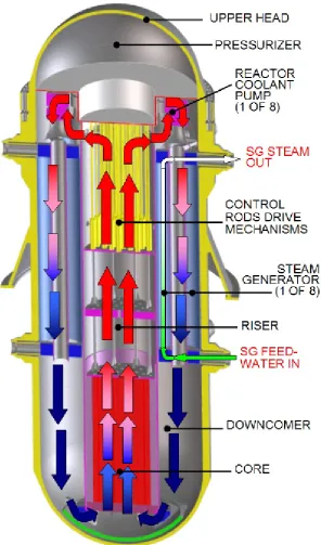
Figure 1. Layout of the IRIS Primary System ... 3

Figure 2. Pressurizer Heater Output ... 10

Figure 3. Primary Pressure ... 11

Figure 4-1. Chi-Squared Values for the Primary Side of the System for the 10% Step Load Change ... 11

Figure 4-2. Chi-Squared Values for the Secondary Side of the System for the 10% Step Load Change ... 12

Figure 5-1. Chi-Squared Values for the Primary Side of the System for the Uncontrolled Rod Bank Withdrawal obtained with Inactive Controllers... 13

Figure 5-2. Chi-Squared Values for the Primary Side of the System for the Uncontrolled Rod Bank Withdrawal obtained with Inactive Controllers... 13

Figure 6-1. Chi-Squared Values for the Primary Side of the System for the Uncontrolled Rod Bank Withdrawal obtained with Active Controllers ... 14

Figure 6-2. Chi-Squared Values for the Secondary Side of the System for the Uncontrolled Rod Bank Withdrawal obtained with Active Controllers... 14

Figure 7. Chi-Squared Values for the Secondary Side of the System for the 10% Step Load Change ... 42

Figure 8. Pressurizer Setpoints ... 54

Figure 9. Standard Deviations for the Input Parameters for Experiment A at 80% Power ... 66

Figure 10. Standard Deviations for the Input Parameters for Experiment B ... 66

Figure 11. Standard Deviations for the Input Parameters for Experiment C ... 67

Figure 12. Standard Deviations for the Input Parameters for Experiment D ... 67

Figure 13. Standard Deviations for the Input Parameters for Experiments A, B, C and D ... 68

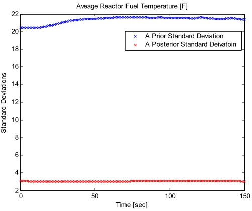
Figure 14-1. Standard Deviations for Average Fuel Temperature for RCP Trip using Experiment A at 80% Power for Data Assimilation ... 69

Figure 14-2. Standard Deviations for Hot Channel Fuel Centerline Temperature for RCP Trip using Experiment A at 80% Power for Data Assimilation ... 69

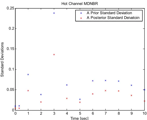
Figure 14-3. Standard Deviations for Hot Channel MDNBR for RCP Trip using Experiment A at 80% Power for Data Assimilation... 70

Figure 15-1. Standard Deviations for Average Fuel Temperature for Control Bank Withdrawal using Experiment B for Data Assimilation ... 70

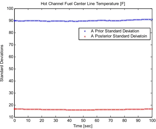
Figure 15-2. Standard Deviations for Hot Channel Fuel Centerline Temperature for Control Bank Withdrawal using Experiment B for Data Assimilation... 71

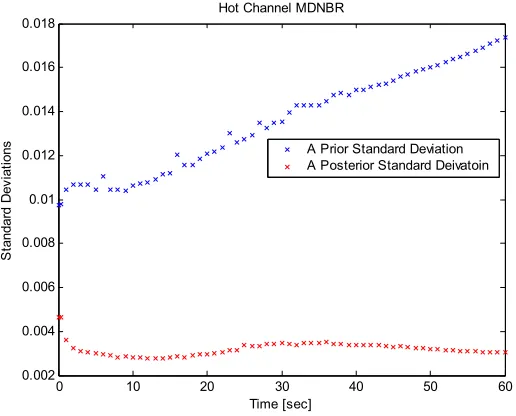
Figure 15-3. Standard Deviations for Hot Channel MDNBR for Control Bank Withdrawal using Experiment B for Data Assimilation ... 71

Figure 16-2. Standard Deviations for Hot Channel Fuel Centerline Temperature for FCV Failed Open using Experiment C for Data Assimilation ... 72 Figure 16-3. Standard Deviations for Hot Channel MDNBR for FCV Failed Open using

Experiment C for Data Assimilation... 73 Figure 17-1. Standard Deviations for Average Fuel Temperature for TCV Failed Open

using Experiment D for Data Assimilation... 73 Figure 17-2. Standard Deviations for Hot Channel Fuel Centerline Temperature for TCV

Failed Open using Experiment D for Data Assimilation ... 74 Figure 17-3. Standard Deviations for Hot Channel MDNBR for TCV Failed Open using

Experiment D for Data Assimilation ... 74 Figure 18-1. Standard Deviations for Average Fuel Temperature for RCP Trip using

Experiment A, B, C and D for Data Assimilation ... 75 Figure 18-2. Standard Deviations for Hot Channel Fuel Centerline Temperature for RCP

Trip using Experiment A, B, C and D for Data Assimilation... 75 Figure 18-3. Standard Deviations for Hot Channel MDNBR for RCP Trip using

Experiment A, B, C and D for Data Assimilation ... 76 Figure 19-1. Standard Deviations for Average Fuel Temperature for Control Bank

Withdrawal using Experiment A, B, C and D for Data Assimilation... 76 Figure 19-2. Standard Deviations for Hot Channel Fuel Centerline Temperature for Control Bank Withdrawal using Experiment A, B, C and D for Data Assimilation ... 77 Figure 19-3. Standard Deviations for Hot Channel MDNBR for Control Bank Withdrawal

using Experiment A, B, C and D for Data Assimilation... 77 Figure 20-1. Standard Deviations for Average Fuel Temperature for FCV Failed Open

using Experiment A, B, C and D for Data Assimilation... 78 Figure 20-2. Standard Deviations for Hot Channel Fuel Centerline Temperature for FCV

Failed Open using Experiment A, B, C and D for Data Assimilation ... 78 Figure 20-3. Standard Deviations for Hot Channel MDNBR for FCV Failed Open using

Experiment A, B, C and D for Data Assimilation ... 79 Figure 21-1. Standard Deviations for Average Fuel Temperature for TCV Failed Open

using Experiment A, B, C and D for Data Assimilation... 79 Figure 21-2. Standard Deviations for Hot Channel Fuel Centerline Temperature for TCV

Failed Open using Experiment A, B, C and D for Data Assimilation ... 80 Figure 21-3. Standard Deviations for Hot Channel MDNBR for TCV Failed Open using

Experiment A, B, C and D for Data Assimilation ... 80

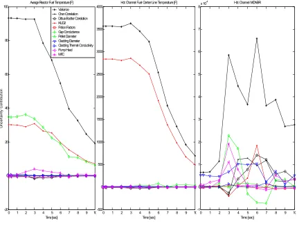
Figure 22. Each Parameter’s Uncertainty Contribution to the System Attributes for RCP

Trip... 82

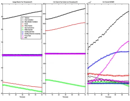
Figure 23. Each Parameter’s Uncertainty Contribution to the System Attributes for

Control Bank Withdrawal ... 83

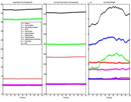
Figure 24. Each Parameter’s Uncertainty Contribution to the System Attributes for FCV

Failed Open... 84

Figure 25. Each Parameter’s Uncertainty Contribution to the System Attributes for TCV

Figure 26. Each Parameter’s Uncertainty Contribution to the System Attributes for RCP Trip as a Result of Multiple Experiments ... 86

Figure 27. Each Parameter’s Uncertainty Contribution to the System Attributes for

Control Bank Withdrawal as a Result of Multiple Experiments ... 87

Figure 28. Each Parameter’s Uncertainty Contribution to the System Attributes for FCV

Failed Open as a Result of Multiple Experiments ... 88

Figure 29. Each Parameter’s Uncertainty Contribution to the System Attributes for TCV

Failed Open as a Result of Multiple Experiments ... 89 Figure 30. Accepted Input Parameter Vector Samples ... 91 Figure 31. A posteriori distribution of the parameters using RCP Trip at 30% Power.... 92 Figure 32. A posteriori distribution of the parameters using RCP Trip at 80% Power.... 95 Figure 33. Inner Optimization using A Priori Design Margin ... 100

Figure 34. Constraint Violation for Inner Optimization using A Priori Design Margin 101

Figure 35. Inner Objective Function using All Experiments and Sensors for Data

Assimilation ... 101

Figure 36. Constraint Violation for Inner Objective Function using All Experiments and

Sensors for Data Assimilation ... 102 Figure 37. Objective Function for Outer Iteration ... 103

Figure 38. System Responses obtained Simulating 100 Samples for 10% Step Load

Changes at 70% Power using Control Algorithm F1Q1 for Uncertainty

Analysis... 109

Figure 39. System Responses obtained Simulating 100 Samples for 10% Step Load

Changes at 70% Power using Control Algorithm F3Q1 for Uncertainty

Analysis... 110

Figure 40. System Responses obtained Simulating 100 Samples for 20% Ramp Load

Changes at 70% Power using Control Algorithm F1Q1 for Uncertainty

Analysis... 111

Figure 41. System Responses obtained Simulating 100 Samples for 20% Ramp Load

Changes at 70% Power using Control Algorithm F3Q1 for Uncertainty

1. Introduction 1. 1. Overview of the IRIS Reactor System

IRIS (International Reactor Innovative and Secure) reactor system has been developed by an

international consortium of twenty plus organization from nine countries with the original

purpose of commercially deploying it in the next decade, but has since been abandoned. It is

a 1000 MWt integral PWR which has eight helical steam generators, eight spool-type pumps,

neutron reflector, pressurizer and control rod drive mechanism inside the reactor vessel [1].

The current design features of this small scale advanced light water reactor’s vessel are

presented in Figure 1. The primary system is contained in the reactor vessel and reactor

coolant is pumped in a closed circuit in the vessel. The coolant goes up through the core,

turns outward at the top of the internal, flows up to the eight primary pumps, is pumped

downward through the pumps and through the steam generators, down the annulus between

the core barrel and the reactor vessel wall, then upward through the core support assembly.

Steam generator (SG) feedwater passes through the feedwater nozzles into the feedwater

header, enters the steam generator tube and flows upward inside the tubes, first being heated

to saturation, then boiled, and subsequently heated to dry superheated steam, which then

flows into the upper steam discharge header and out through the steam outlet nozzles to the

turbines. Both the SG feedwater and steam headers attach directly to the reactor vessel inside

wall and form the primary to secondary pressure boundary.

One of the primary goals of the IRIS project is to complete the “safety by design.” First of all,

piping of conventional PWRs does not exist. This is the unique characteristic of the Small

Modular Reactor (SMR). The large vessel per unit thermal energy compared to other PWRs

provides a large coolant inventory in the reactor coolant system, which contributes to the

more favorable IRIS responses to small and medium LOCAs. The large coolant inventory per

unit thermal energy also provides a large heat sink that acts to effectively mitigate cooldown

and heatup events. The IRIS once through steam generators with the primary coolant on the

shell side provide reduced probability and consequences of the steam generator tube rupture

accident. Another feature of IRIS once through steam generators is the limited secondary side

water inventory, which reduces the consequences of cooldown event, e.g. steam line break.

However, on the other hand, the limited inventory on the secondary side provides less

mitigation to heatup events, e.g. feed line break. In this case, the large volume of the

pressurizer compensates for the limited heat sink provided by the steam generators (The

steam volume to reactor power ratio is five times larger in IRIS than in advanced passive

PWRs). It is also obvious that multiple coolant pumps and steam generators mitigate single

component failure accidents for the IRIS. As it is presented above, the primary goal of the

1. 2. Motivation

Estimating nuclear reactor performance during a transient has been the main issue in thermal

hydraulic safety research since nuclear energy was first used to produce electricity. For the

IRIS reactor that may be built and operated for the first time, simulation models have been

developed and tested for the safety research using multiple thermal-hydraulic equations

coupled to each other [2], [3]. The quality of the plant system simulator predictions will

impact the reactor economy through the introduction of margins on the reactor design to

ensure an operation, in which the safety and operational limits are satisfied with a high

degree of certainty. How tight or relaxed these margins are depends on how accurate the

predictions of reactor behavior are. The uncertainties of reactor simulator calculations are

thus important to the determination of these margins. The IRIS research has been focused on

a design that provides the highest degree of safety and cost effective arrangement. That is, by

reducing uncertainties, safety can be maintained while costs are reduced.

The fidelity of the prediction cannot be evaluated directly unless the validation is performed

using suitable measurements in nuclear plants. A great deal could be learned from

experimental data to enhance simulation fidelity for a nuclear reactor. In particular, input

parameters can be refined assuming it is the major source of uncertainties. Using adjusted

thermal hydraulic input parameters and their reduced uncertainties, subsequent reactor

simulation improves the prediction of key system attributes. The objective of this work is to

reduce the uncertainties on limiting system attributes during accident transients. To

complete data assimilation on the thermal-hydraulic input parameters to the system

simulation code, in our case the IRIS system simulator. This was done by using the

IRISN.Ver08.Mod06 [2] simulator developed at NC State to complete virtual experiments

and generate their associated experimental data. This code predicts the performance of the

IRIS reactor by solving multiple thermal hydraulic equations for both the primary and the

secondary systems. The primary side responses, e.g. pressure, temperature, coolant flow rate,

etc., are calculated based on the mass, momentum and internal energy equations, which are

introduced in Appendix B. Historical research on the thermal hydraulic reactor system

indicates that the system responses are usually nonlinear, which adds complexity to data

assimilation. To determine whether the nonlinearities would exist for experiments performed

at lower power initial conditions, and if so, utilize a data assimilation method capable of

addressing nonlinearity, IRIS system simulations can be completed.

1. 3. Literature Review

The uncertainty and sensitivity analysis for the thermal hydraulic reactor system has been

widely performed for the uncertainty evaluation of the best estimate LOCA analysis. The

best estimate plus uncertainty (BEPU) method was introduced and developed in the 1980s to

support licensing. The code scaling, applicability, and uncertainty (CSAU) evaluation

method was subsequently developed for application to the LBLOCA in a pressurized water

reactor [4]. The CSAU methodology contains 14 steps organized into three major elements:

Requirements and Code Capabilities, Assessment and Ranging of Parameters, and Sensitivity

included development of the embedded Phenomena Identification & Ranking Table (PIRT)

methodology. The PIRT has become a standard accepted throughout the international nuclear

community providing guidance in executing cost effective BEPU applications. In 1996, the

USNRC approved a best estimate loss of coolant accident method based upon CSAU and the

WCOBRA/TRAC thermal hydraulic code. Since the first uncertainty analysis performed

with the CSAU method, several different methods have been proposed for uncertainty and

sensitivity analysis. One of them is Uncertainty Analysis Methodology based on Accuracy

Extrapolation (UMAE) which addresses model validation [5]. It is based on the extrapolation

of the accuracy resulting from a comparison between the code predictions and the

experimental data obtained in small scale facilities. Westinghouse developed a new BEPU

method called Automated Statistical Treatment of Uncertainty Method (ASTRUM) which

was approved in 2004 [6]. The ASTRUM is still based on the WCOBRA/TRAC thermal

hydraulic code but it utilizes a non-parametric (distribution free) statistical sampling

technique. Since it eliminates the superposition penalty associated with employing a surface

response surrogate model, this technique is expected to reduce the predicted Peak Cladding

Temperature (PCT). The BEMUSE (Best Estimate Method – Uncertainty and Sensitivity

Evaluation) phase 3 benchmark assesses the reliable application of high quality best estimate

and uncertainty and sensitivity evaluation methods [7]. It shows the method and results of the

peak cladding temperature estimation conducted by ten participants from nine organizations

and seven countries. The main characteristic of the approach used by participants is the

propagation of the input parameters’ uncertainties relying on probabilistic analysis associated

In Monte Carlo analysis, a probabilistic based sampling is used to develop a mapping from

input parameters to system responses. Several possible sampling methods exist, including

simple random sampling, stratified sampling and Latin Hypercube Sampling (LHS). Due to

demanding calculation requirements, the Monte Carlo method is usually not applicable,

particularly for data assimilation, to a large scale thermal hydraulic system simulation code.

For the neutronic problem, a more deterministic approach has been used for the BEPU

analysis. In order to deal with the reactor physics problem that has many more parameters

than the thermal hydraulic problem has, adjoint sensitivity analysis was developed to reduce

the calculational effort [8]. The adjoint method is known to be very powerful for a system

that has multiple input parameters and a few responses, but sometimes inapplicable for the

large scale thermal hydraulic system due to nonlinearity of the responses over their ranges of

uncertainties. The Efficient Subspace Method (ESM) has also been developed for the

neutronic problem utilizing Singular Value Decomposition (SVD) to deal with ill

conditioned matrices [9], [10]. It was specifically developed for data assimilation for

problems with both large parameter and response fields. Nowadays BEPU methods are

widely used in the world and the industry is more focusing on development of new licensing

BEPU methods. Even though many papers deal with the uncertainty evaluation methods,

none of them presents the method which tremendously reduces the computing demand for

thermal hydraulic system calculations. In addition, limited research has been conducted to

system associated with a power reactor, which can possibly reduce a posteriori uncertainties

of the system attributes.

The work reported here presents data assimilation capabilities combined with an optimization

technique developed to determine near-optimum thermal hydraulic experiments to perform

on IRIS to minimize uncertainties in limiting reactor responses. This capability was

developed such that the IRIS design was at the same time reoptimized to utilize the margin

introduced. In chapter 2, the description of this analysis is presented. The methods that solve

the nonlinear system based on the virtual experimental model using both deterministic and

probabilistic methods are presented in sections 2.1 through 2.5. In section 2.6, the

optimization methodology used to design the thermal hydraulic system of the IRIS is

discussed. Following the discussion, the uncertainty analysis technique for the reactor control

problem is presented in section 2.7. In chapter 3, results of data assimilation, optimization,

and uncertainty analysis for the reactor control are provided to show the optimum design of

the IRIS reactor achieved by reduced uncertainties on the reactor system. Following the

results, conclusions and recommendations for future work are outlined in chapter 4. Finally,

this dissertation includes appendices A and B providing several mathematical derivations.

Appendix A shows the mathematical approach for data assimilation incorporating the

parameter-response covariance matrix. In appendix B, the physical models for the primary

side of the reactor are introduced, and the mathematical derivations for the numerical

2. Description of the Actual Work 2. 1. Linearity Test for the IRIS Reactor System

Since the preferred method for data assimilation and uncertainty quantification is dependent

upon whether the observables, i.e. sensor signals, and attributes, e.g. Departure from

Nucleate Boiling Ratio (DNBR), sensitivity equations are nearly linear or not, a Chi-Square

test is required to confirm the system sensitivity equations linearity. For the Chi-Square

goodness of fit, the observables and system attribute data are divided into K bins and the test

statistic is defined as:

(

)

2

1 K

i i

i i

O E

E χ

= −

=

∑

where O_i is the observed frequency for bin i and E_i is the expected frequency for bin i. If

the sensitivity equations are linear and the parameters uncertainty distributions are Gaussian,

the sensor and attribute distributions will also be Gaussian. Thus using a Gaussian

distribution to obtain values for E_i and the IRIS simulator to obtain values of O_i, Chi-Square values can be obtained for the observables and attributes. One observes that not all

observables and/or system attributes are within the desired level of the Chi-Square value, i.e.

acceptable range of the linearity, if the reactor controllers are on and/or the transient is rapid.

The reactor controllers that are associated with safety systems control certain observables,

e.g. primary pressure, causing the reactor system to not behave naturally, which results in

nonlinearity. Obviously the rapidness of the transients also causes the nonlinearity, e.g. RCP

Trip. Note that the safety controllers, e.g. pressurizer heaters and feedwater controllers, could

change. For further discussion of the Chi-Squared test, all of the samples are combined and

presented in Figures 2 for a 10% step load change simulation. In order to see the impact of

the pressurizer heaters on the system, all important control systems were turned off except

the feedwater controllers and the pressurizer heaters. Figure 2 indicates that the pressurizer

heater, which has a limited capacity as constrained by output capacity, is active during the

transient. This causes nonlinearity in the primary pressure as shown in Figure 3 and 4-1.

Some of the responses of the observables on the primary side could be affected by this

nonlinearity as well. Since the minimum DNBR is a strong function of the system pressure,

core flow rate, and coolant temperature, the hot channel minimum DNBR also shows

nonlinearity. Similar to the safety control mechanism that produces a nonlinear primary

pressure response, active feed pumps and feed control valves actions during the step load

change result in nonlinearity that appears especially on the secondary side of the reactor

system as shown in Figure 4-2.

0 50 100 150 200 250

0 200 400 600 800 1000 1200 1400

Time [sec]

P

re

ss

ur

iz

er

P

rop

or

tion

al

H

ea

ter

O

ut

put

[

M

w

]

0 50 100 150 200 250 2210

2220 2230 2240 2250 2260 2270

Time [sec]

P

rim

ar

y P

res

su

re

[

ps

ia]

Figure 3. Primary Pressure

0 50 100 150 200 250

0 50 100 150 200 250

Time [sec]

C

hi

S

quar

ed

V

al

ues

Neutron Power

Reactor Thermal Output Core Flow Rate

Primary Pressure Hot Leg Temperature Cold Leg Temperature Average Coolant Temperature 5% Level Chi-Square Value

Figure 4-1. Chi-Squared Values for the Primary Side of the System for the 10% Step Load

0 50 100 150 200 250 0

50 100 150

Time [sec]

C

hi

Sq

ua

re

d

Va

lu

es

Feed Flow Rate Steam Flow Rate Turbine Output

Steam Generator Exit Temperature Steam Pressure

5% Level Chi-Square Value

Figure 4-2. Chi-Squared Values for the Secondary Side of the System for the 10% Step Load

Change

In order to simulate natural responses of the reactor system, IRIS simulations for several

transients assuming inactive reactor controllers were completed for 100 samples of the

parameters using Latin Hypercube sampling. Figure 5 illustrate the Chi-Squared values of the

observables as a function of time for the uncontrolled rod bank withdrawal transient. With

the safety controller, e.g. pressurizer heaters, as well as the reactor system controllers

assumed to be turned off, the reactor system behaves naturally and the Chi-Square values for

most observables and the system attributes decrease versus if these controllers are on (see

0 10 20 30 40 50 60 0

5 10 15 20 25 30

Time [sec]

C

hi

S

qua

re

d

V

al

ue

s

Neutron Power Reactor Thermal Output Core Flow Rate Primary Pressure Hot Leg Temperature Cold Leg Temperature Average Coolant Temperature 5% Level Chi-Square Value

Figure 5-1. Chi-Squared Values for the Primary Side of the System for the Uncontrolled Rod

Bank Withdrawal obtained with Inactive Controllers

0 10 20 30 40 50 60

0 5 10 15 20 25

Time [sec]

C

hi

S

quare

d

V

al

ues

Feed Flow Rate Steam Flow Rate Turbine Output

Steam Generator Exit Temperature Steam Pressure

5% Level Chi-Square Value

Figure 5-2. Chi-Squared Values for the Secondary Side of the System for the Uncontrolled

0 10 20 30 40 50 60 0

20 40 60 80 100 120 140 160 180

Time [sec]

C

hi S

qu

ar

ed

V

alu

es Neutron Power

Reactor Thermal Output Core Flow Rate Primary Pressure Hot Leg Temperature Cold Leg Temperature Average Coolant Temperature 5% Level Chi-Square Value

Figure 6-1. Chi-Squared Values for the Primary Side of the System for the Uncontrolled Rod

Bank Withdrawal obtained with Active Controllers

0 10 20 30 40 50 60

0 10 20 30 40 50 60

Time [sec]

C

hi

S

qua

re

d V

al

ues

Feed Flow Rate Steam Flow Rate Turbine Output

Steam Generator Exit Temperature Steam Pressure

5% Level Chi-Square Value

Figure 6-2. Chi-Squared Values for the Secondary Side of the System for the Uncontrolled

2. 2. Data Assimilation and Uncertainty Quantification

2.2.1. Deterministic Method for the Mildly Nonlinear Problems

Nuclear power plant design and operation must accommodate the uncertainties in predicting

system performance, those uncertainties originated due to initial conditions, parameters,

numerics and modeling uncertainties. Assuming that parameters’ uncertainties are the major

contributors to observables and attribute uncertainties compared to any other sources of

uncertainties, they can be refined to develop a higher fidelity model. Using adjusted thermal

hydraulic parameters and their reduced uncertainties, subsequent reactor simulation improves

the prediction of key system attributes if closely related to the system observables. In order to

accomplish this, given measurements of the observables and a priori distributions of the

parameters, one solves an inverse problem adjusting the parameter values to achieve better

agreement between measured and predicted sensor response values [11]. Since IRIS is not

operational anywhere, to generate the experimental values of the observables a virtual reactor

is employed. By this is implied that a computer simulation is used to predict the experimental

values, where perturbed parameter values have been used that are consistent with their

uncertainties.

The distribution of the parameters (assumed Gaussian), whose mean is p₀ and whose

covariance matrix is Cp, is given by:

{

} {

}

T

1 T 1

0 0

1 1 0 0

0 0

1 1

( ) exp exp

2 p 2 p

p p p p

p C C C p p C p p

p p

ρ = ⎡⎢− ⎧_⎨⎪ − ⎪⎫_⎬ − ⎧⎪_⎨ − ⎫⎪_⎬⎥⎤= _⎢⎡− − − − ⎤_⎥

⎢ ⎪⎩ ⎪⎭ ⎪⎩ ⎪⎭⎥ ⎣ ⎦

⎣ ⎦

where p≡ p p₀ implying p are relative values with respect to the a priori parameters value, and p₀ is the unit vector. The constant C₁ serves as the normalization constant valued such the ρ( )p when integrated over all p values equals 1.0. Note that an overline indicates a vector and a double overline denotes a matrix. In general, the expectation of function (x)f ,

denoted as f(x) , is defined as:

x

(x) (x) (x) x

S

f ≡

∫

where S_x represents the space formed by all possible values of x . (x)P is recognized as a

joint probability density function. The first moment, i.e. (x) xf = , renders the mean value,

and the second moment, i.e. f(x)=_⎣⎡x− x _{⎦ ⎣}⎤ ⎡x− x ⎤_⎦T, renders the covariance matrix.

Using these generalized definitions, the a priori parameter covariance matrix is defined as

follows:

T T

0 0 0 0 ( )

p

prior p

S

C ≡ _⎣⎡p p− ⎤ ⎡_{⎦ ⎣}p p− ⎤_⎦ =

∫

where S_p is the parameter space.

The sampling model for the observations whose uncertainties can be represented by a

Gaussian probability distribution centered at r and with experimental uncertainty covariance

{

} {

}

2

1

( | ) exp

2

m m m m

r r C r r C r r

ρ = ⎡_⎢− − − − ⎤_⎥

⎣ ⎦ (2.5)

where, rm and r denote the virtual experiment sensor signal vector and the mean value vector (taken as the design (simulator) model prediction vector), respectively, with the

pdependence of rsuppressed. The constant C₂ is again the normalization constant. In this

work, Cm is assumed diagonal and variance values set to those typical of nuclear power plant sensors. Note that to obtain the virtual reactor sensor signals accounting for observation

uncertainty, observation errors are applied to the virtual reactor simulators predicted signal

values, rm. The virtual experiments that were modeled are presented in section 2.3. For J distinct sensors and Tdiscrete times each system response vector rj can be represented as follows:

{

}

j _j

r = r t= T (2.6)

Then the vector r which contains all of the system responses is: T

T T T

1 2 J

r_{= ⎢}⎡r r r ⎤_⎥

⎣ … ⎦ (2.7)

If the system is linear or mildly nonlinear, the design model can be linearized by the

following first-order Taylor series expansion:

( )

( )

0 0

0 0

( )

p p

where

( )

0

p

S is the time dependent sensitivity matrix computed about the nominal value of

the a priori parameters and δp p p− ₀. Using the a priori distribution of the parameters, the a priori system attribute covariance can be calculated by the sandwich rule as follows:

( )

( )

( )

( )

a p a

p p

C a a a a

a a a a

S p p S

S C S

δ δ ⎡ ⎤ ⎡ ⎤ ≡ _⎣ − _{⎦ ⎣} − _⎦ ⎡ ⎤ ⎡ ⎤ = _⎣ − _{⎦ ⎣} − _⎦ = = (2.9)

where

( )

( )

0 0

0 0

( ) a a

p p

a a p≅ + S δp a= + S δp

Following the Bayesian approach, a posteriori distribution for the parameter vector p is then given by:

{

} {

} {

} {

}

3 0 0

( | ( )) ( ) ( | ) ( ) ( | ) ( ) ( | ) 1

exp ( ) ( )

2 p m m m m m S

m m m p

r r p p

p r

r

r p p

r p d p

C r r p C r r p p p C p p

ρ ρ ρ ρ ρ ρ ρ − − × = × = ⎡ ⎛ ⎞⎤ = _⎢− _⎜ − − + − − _⎟⎥ ⎝ ⎠ ⎣ ⎦

∫

In order to determine the parameter vector that maximizes the Gaussian distribution, i.e. the

mean values of the parameters, the parameter vector that minimizes the following expression

{

} {

} {

} {

}

0 0

( ) ( )

m m m p

r r p C− r r p p p C− p p

⎡ _{− − + − −} ⎤

⎢ ⎥

⎣ ⎦ (2.11)

In general, the minimization problem can be formulated with the parameter-response

combined vector z and the corresponding block covariance matrix C as follows [12]:

0

m

p p z

r r

⎡ − ⎤

≡ ⎢ ⎥

−

⎢ ⎥

⎣ ⎦ ,

p pr

rp m

C C

C

C C

⎡ ⎤

⎢ ⎥

=

⎢ ⎥

⎣ ⎦

(2.12)

where, Cpr =CTrp is the parameter-response covariance matrix. This correlation occurs due to the successive linearization iterations one utilizes in solving the weakly nonlinear data

assimilation problem, associated with updating the observables sensitivity matrix as updated

parameter values become available. If the a priori distribution for the parameters and for the

sampling model can be represented by a Gaussian distribution and the system responses are

linear to the parameters, then the Gaussian probability density function describes the

posteriori uncertainty of p.

1 T 1

( | ) exp

2 m

p r const z C z

ρ = ⋅ ⎧_⎨− − ⎫_⎬

⎩ ⎭ (2.13)

The mathematical approach for this analysis is presented in Appendix A. Since the

thermal-hydraulic reactor system model is not highly nonlinear, the a posteriori parameters approach

the converged solution quickly and their uncertainties significantly decrease after the first

iteration. This makes the parameter adjustments associated with the second linearization

iteration small; furthermore, significantly reduced uncertainties of the parameters after the

first iteration will cause small parameter-response uncertainties as well. Thus, adding the

thermal-hydraulic inverse problem [13]. Solution to the minimization problem is then accomplished

by differentiating expression (2.11) with respect to p.

Generalizing, the problem can also include a regularization parameter, α , to address any

ill-conditioning and to control the amount of parameter adjustments allowed. Thus the

minimization problem becomes:

{

} {

} {

} {

}

0 0

min m ( ) m m ( ) p

p r r p C r r p α p p C p p

− −

⎡ _{− − + − −} ⎤

⎢ ⎥

⎣ ⎦ (2.14)

The first term in this equation is the mismatch term between the virtual experiment sensor

readings and the design model predictions. The second term in the equation is the

regularization term, which shows the change in a priori to a posteriori values of the

parameters with respect to the matrix norm of the parameters covariance matrix. Tikhonov

regularization [14] was employed, where the weighting sum of the mismatch term and

regularization term is minimized by selection of the posteriori input parameter values. The

regularization parameter indicates the degree of weighting between the mismatch term and

the regularization term. For large α values, a posteriori parameter values will not deviate

greatly from their a priori values. This implies the mismatch term will not be reduced very

much by data assimilation. For small alpha values, the reverse behavior occurs. The

Tikhonov regularization parameter was selected experimentally based on the characteristic

L-curve [15]. For a Bayesian approach, one would set α =1 to produce unbiased a posteriori

values. Assuming linearity of the sensitivity equations, the a posteriori parameter vector is

1

T 1 1 T 1

2

0

0 0

post

m

m p m

p p S C S α C S C r r

−

− − −

⎡ ⎤ _{⎡ ⎤}

= +_⎢ + _{⎥ ⎣} − _⎦

⎣ ⎦ (2.15)

and a posteriori system responses and attributes are given as:

( )

( )

post post post post post

p p

r ≅r p + S δp =r + S δ p (2.16)

and

( )

( )

0 0

0 0

( ) _{post post}

post post post post post

a a

p p

a ≅a p + S δp =a + S δ p (2.17)

respectively. The a posteriori parameter covariance matrix can be also computed by:

T

0 0

post _{post post}

p

C ≡ ⎡_⎢⎣p p− ⎤ ⎡_{⎥ ⎢⎦ ⎣}p p− ⎤_⎥⎦ (2.18)

Substituting Equation (2.15) for the posteriori parameters into Equation (2.18) produces the

following expression for Cpostp :

{

}

{

}

{

}

{

}

1

T 1 1 T 1

2

0 0

T 1

T 1 1 T 1

2 0 0 post m

p m p m

m

m p m

C p p S C S C S C r r

p p S C S C S C r r

(

)

(

)

(

)

T

T 1 T 1 1

2

0 0

1

T 1 ₂ 1 T 1 T

0 0

1

T 1 1 T 1

2 0 prior m

p m m p

m

m p m

m p m

m m

C p p r r S p p C S S C S C

S C S C S C r r S p p p p S C S C S C

r r S p p r

α α α − − − − − − − − − − − − ⎡ ⎤ ⎡ ⎤ ⎡ ⎤ = − _⎣ − _{⎦ ⎢⎣} − + − _{⎥⎦ ⎢} + _⎥ ⎣ ⎦ ⎡ ⎤ _{⎡ ⎤ ⎡ ⎤} −_⎢ + _{⎥ ⎢} − + − _⎥⎣ − _⎦ ⎣ ⎦ ⎣ ⎦ ⎡ ⎤ +_⎢ + _⎥ ⎣ ⎦ ⎡ ⎤

× _⎢⎣ − + − _⎥⎦

(

)

T

1 T 1 1

2

m m p

r S p p C S S C S α C

− − − − ⎡ _{− + −} ⎤ ⎢ ⎥ ⎣ ⎦ ⎡ ⎤ × _⎢ + _⎥ ⎣ ⎦ (2.19) T

T 1 T 1 1

2

1

T 1 1 T 1

2

1

T 1 1

2

T 1 T

prior prior prior

p pr p m m p

prior prior

m p m rp p

prior

m p

m m rp pr

C C C S C S S C S C

S C S C S C C SC

S C S C

S C C C S SC SC

α α α − − − − − − − − − − − − ⎡ ⎤ ⎡ ⎤ = +_⎢ − _{⎥ ⎢} + _⎥ ⎣ ⎦ ⎣ ⎦ ⎡ ⎤ ⎡ ⎤ +_⎢ + _{⎥ ⎢} − _⎥ ⎣ ⎦ ⎣ ⎦ ⎡ ⎤ +_⎢ + _⎥ ⎣ ⎦

× − − + T 1

T

T 1 1

2 prior p m prior m p

S C S S C S α C

− − − − ⎡ ⎤ ⎢ ⎥ ⎣ ⎦ ⎡ ⎤ ×_⎢ + _⎥ ⎣ ⎦ T 1

T 1 T 1 1 T 1 1 T 1

2 2

1 T

T 1 1 T 1 T 1 T 1 1

2 2

prior prior prior prior prior

p p m m p m p m p

prior prior prior

m p m m p m m p

C C S C S S C S C S C S C S C SC

S C S C S C C SC S C S S C S C

α α α α − − − − − − − − − − − − − − − − ⎡ ⎤ ⎡ ⎤ ≅ − _⎢ + _⎥ −_⎢ + _⎥ ⎣ ⎦ ⎣ ⎦ ⎡ ⎤ ⎡ ⎤ ⎡ ⎤ +_⎢ + _{⎥ ⎢} + _{⎥ ⎢} + _⎥ ⎣ ⎦ ⎣ ⎦ ⎣ ⎦

As noted earlier, to address mild nonlinearity, sensitivity coefficient values were

redetermined linearizing about the previous iteration a posteriori parameter values, and

inverse theory was once again used to obtain updated a posteriori parameters values. These

Best-estimate accident analysis requires not only values of limiting system attributes during

accident transients, e.g. Minimum Departure from Nucleate Boiling Ratio (MDNBR), but

also their uncertainties. To obtain those, given a posteriori parameter uncertainties, one can

propagate the parameter uncertainties through the simulation model to predict a posteriori

uncertainties on core observables and system attributes. If the a posteriori parameter

uncertainties are Gaussian and the system responds linearly over the range of the parameter

uncertainties, the system attribute uncertainties are Gaussian, which is characterized by the

mean values and covariance at the operating power level for the accident “acc” given by:

0 0

T

post post

o o o

acc post acc post acc

a a p a

p p

C S C S

⎛ ⎞ ₌⎛ ⎞ ⎛ ⎞

⎜ ⎟ ⎜ ⎟ ⎜ ⎟

⎝ ⎠ ⎝ ⎠ ⎝ ⎠ (2.20)

where

( )

nonlinear, one should propagate parameter uncertainties by Monte Carlo simulation. As done

in this work, data assimilation was completed using experiments conducted mostly at lower

powers, since experiments actually corresponding to higher power accident conditions would

be prohibited. In this case, one should always pay attention to the similarity of physics. If the

physics at operating power is significantly different from that at lower power, the calculated

a posteriori system attribute uncertainty would in general not represent that associated with

the actual transient starting at operating power. Thus the similarity of physics should always

Literature reviews were completed to identify the uncertainties on parameters and

correlations within the model, and which system responses and attributes would need to be

considered. The following parameters/correlations [4], [17], [18], [19] were selected to have

their values adjusted via data assimilation:

1. Chen Heat Transfer Correlation for nucleate boiling heat transfer coefficient on the

secondary side of steam generator

2. Dittus-Boelter Heat Transfer Correlation for single phase (liquid or gas) heat transfer

coefficient on the secondary side of steam generator

3. Fuel Thermal Conductivity

4. Friction Factors

5. Gap Conductance

6. Pellet Diameter

7. Cladding Diameter

8. Cladding Thermal Conductivity

9. Pump Head (RCP and FP)

10. Moderator Temperature Coefficient

The following observables were selected for usage during data assimilation:

1. Neutron Power

2. Reactor Thermal Output

3. Core Flow Rate

4. Primary Pressure

6. Cold Leg Temperature

7. Average Coolant Temperature

8. Feed Flow Rate per Steam Generator

9. Steam Flow Rate per Steam Generator

10. Turbine Output

11. Steam Generator Exit Temperature

12. Steam Pressure

In addition the following system attributes were selected for uncertainty quantification:

1. Average Reactor Fuel Temperature

2. Hot Channel Fuel Center Line Temperature

3. Hot Channel Minimum Departure from Nucleate Boiling Ratio

Table I. Uncertainties of Observables

Observables Measurement Uncertainties (1σ)

Neutron Power 2%

Reactor Thermal Output 2%

Core Flow Rate 2.74%

Primary Pressure 18.2 psia

Hot Leg Temperature 2.43 F

Cold Leg Temperature 2.43 F

Average Coolant Temperature 2.43 F

Feed Flow Rate per Steam Generator 1.6%

Steam Flow Rate per Steam Generator 1.6%

Turbine Output 2%

Steam Generator Exit Temperature 2% (assumed)

Table I presents the sensors’ uncertainties employed, which are based upon the

instrumentation used in operating PWRs [30]. In addition, calculations were also completed

using a larger uncertainty on core flow rate, 6%, since it was judged that with an integral

PWR this uncertainty would be larger than for loop configurated PWR.

2.2.2. MCMC Method for the Nonlinear Problems

All of the above discussion is based upon the parameters and observables uncertainties being

Gaussian and the system sensitivity equations being mildly nonlinear i.e. nearly linear.

However according to the linearity test, nonlinear behaviors were observed at the lower

power experimental condition, especially on the secondary side of the reactor. The

deterministic approach, based upon a first order truncated Taylor series representation for the

responses, to uncertainty analysis is inappropriate to treat this behavior due to the nonlinear

relationship between the system responses and the parameters, hence the potential

non-Gaussian nature of the a posteriori distribution. This provides motivation that the transients

that generate nonlinear system responses be differentiated from those that behave relatively

linearly. To address the nonlinear responses in both data assimilation and determining the a

posteriori uncertainties of the parameters, the following approach was employed.

Following the Bayesian approach, a posteriori distribution for the parameter vector p is then given by Equation (2.10). If the system observables are linear with respect to the parameters,

then solutions to the inverse problem could be obtained analytically as presented in section

transients, given a priori parameter uncertainty information, one needs to propagate the

parameter uncertainties through the simulation model to predict the a posteriori uncertainties

of the parameters using Monte Carlo simulations [20]. This is conducted using the Markov

Chain Monte Carlo (MCMC) method which seeks to determine the steady-state Markov

distribution by generating Markov chains, which coincides with the target distribution, i.e.

the a posteriori distribution of the parameters. A simple MCMC implementation uses the

Metropolis algorithm which is presented as follows:

1. Initialize the parameter vector by guessing it at some value.

2. Given the current parameter vector is pi , generate a new parameter vector p* in

,

i i

p m p m

⎡ _{− +} ⎤

⎢ ⎥

⎣ ⎦, where m is a random number vector.

3. Compute the Metropolis acceptance probability using the following expression:

*

( | )

min 1,

( | )

m i

m

p r p r ρ α

ρ

⎧ ⎫

⎪ ⎪

= _{⎨ ⎬}

⎪ ⎪

⎩ ⎭

4. Define

*

1 with probability

with probability 1 i

i

p p

p

α α

+ ⎧⎪

= ⎨

⎪ −

⎩

selecting which value to assign via a random

number [0,1]

5. Return to step 2.

At the beginning of the sequence, one needs to run MCMC for awhile to achieve

considers a certain number of the first iterations to be discarded as the burn in stage to

remove the bias from the initially chosen starting point. The size of the perturbation, i.e. the

trial space, can be adapted during the burn in phase to a value that provides a desired

acceptance percentage. It has been claimed that, for a wide variety of problems, acceptance

probability near 50% indicates that the chain has good mixing [21], [22], [23]. When the

percentage is less than 30%, i.e. when the trial space is much larger than the target space, the

i

p does not move for long periods, but jumps are large, which implies that one should

perform a large number of simulations to obtain a reasonable number of accepted samples

that illustrate the a posteriori. When the percentage is more than 70%, i.e. when the trial

space is much smaller than the target space, movement across the target pdf is slow, so called

unconstrained random walk, and will not efficiently span the full range of the target

distribution unless the total number of trials is extremely large. In both cases the MCMC

simulation is computationally time consuming since the total number of trials should be

sufficiently large to estimate the a posteriori distribution properly. When simulations do not

provide the desired acceptance percentage, it is possible to improve mixing by properly

adjusting the trial space. Various heuristic rules have been suggested for fixing these

problems during a simulation by monitoring the frequency of acceptances in the simulation.

While the Metropolis algorithm is running, one can monitor the frequency of acceptances of

the Metropolis algorithm; if the acceptance rate is much less or much more than 50%, one

MCMC has proven effective for nonlinear response problems with multiple parameters to

adjust. However this method is not applicable if there are many parameters and the

simulation model requires substantial CPU time to execute due to the computational burden.

2. 3. Virtual Experiments

Data assimilation and uncertainty quantification were completed by defining the

experiments, defining the limiting accidents, and determining the a posteriori uncertainties of

the key system attributes for the limiting accidents. In order to identify the limiting accidents,

the Updated Final Safety Analysis Report (UFSAR) [24] and IRIS Preliminary Safety

Assessment Report [25] were reviewed. Simulations were performed to determine virtual

sensor signals which are surrogates for unavailable experimental values. A single sample of

all the parameter values was used to determine the perturbed parameter values for the virtual

reactor (simulator), from which the virtual reactor sensors’ readings were obtained. In order

to adjust parameters, the following four experiments were simulated using the IRIS system

simulation code.

A. Reactor Coolant Pump (RCP) Trip at 30 % and 80% Power

The simulation is performed for 8 seconds. As mass flow rate decreases below Low Reactor

Coolant Flow Trip Set Point, control rods are inserted and the reactor trips. All control

systems and safety controllers are assumed to be inactive. Note that RCP trip at 80% power

done at relatively high power level to compare the result with that of RCP trip at a lower

power and to minimize computation induced noise from the simulator.

B. Control Bank Withdrawal at 70% Power

The simulation is performed for 60 seconds. The control rod worth was assumed to be

0.893% Δρ. The maximum power reached during the transient is slightly below 845 MWt

which is approximately 85% of the operating power and 113% of the nominal power at 70%

power level. The simulation shows that the reactor does not trip during the experiment since

the large volume of the pressurizer accommodates the primary water volume increase due to

the limited heat sink (The pressurizer steam volume to reactor power ratio is five times larger

in IRIS than in current PWRs). All important control systems are assumed to be inactive

except the control bank.

C. Feed Control Valve (FCV) Failed Open at 15% Power

The simulation is performed for 120 seconds. The feed control valve position is assumed to

experience a +3% step change. All control systems and safety controllers are assumed to be

inactive.

D. Turbine Control Valve (TCV) Failed Open at 15% Power

The simulation is performed for 120 seconds. The turbine control valve position changes

from the initial value of 5% to the final value of 10%. All control systems and safety

2. 4. Uncertainty Contribution to the System Attributes

Since identifying major sources of uncertainty, as done in this work, is important in deciding

where additional efforts should be given to reduce these uncertainties, each parameter’s

uncertainty contribution to the system attributes was determined as well. This was evaluated

for a specific parameter’s uncertainty contribution by determining the system attribute’s

uncertainty propagated from all parameters and subtracting that obtained by propagating

from all but the specific parameter of interest. The associated mathematical derivation is now

given.

Assuming no uncertainty for parameterα_k, the joint distribution function between α_k and α_j is defined using a Dirac-delta function.

(

)

( ,_{k j}) _{k k} ( )_j

P α α =δ α − α Pα (2.21) The ( , )k j elements of a posteriori parameter covariance matrix are then zeros for all js.

(

)

(

)

(

)

,

( ) 0

j k

post

p _{k k j j k k j k j}

S S

k j

C P d d

α α

α α α α δ α α α α α

⎛ _{⎞ = − − − =}

⎜ ⎟

⎝ ⎠

∫ ∫

Likewise

, post p

i k

C

⎛ ⎞

⎜ ⎟

⎝ ⎠ are zeros for all is. Thus the matrix post p

k

C

⎛ ⎞

⎜ ⎟

⎝ ⎠ which does not account for

1,1 1,2 1, 1 1, 1 1,

2,1 2,2 2, 1 2, 1 2,

1,1 1,2 1, 1 1, 1 1,

1,1 1,2 1, 1 1, 1 1,

,1 ,2 , 1 , 1 ,

0 0

0

0 0 0 0 0 0

0

0

k k Np

k k Np

post

k k k k k k k Np

p k

k k k k k k k Np

Np Np Np k Np k Np N

c c c c c

c c c c c

c c c c c

C

c c c c c

c c c c c

− + − + − − − − − + − + + + − + + + − + ⎛ _{⎞ ≡} ⎜ ⎟ ⎝ ⎠ p ⎡ ⎤ ⎢ ⎥ ⎢ ⎥ ⎢ ⎥ ⎢ ⎥ ⎢ ⎥ ⎢ ⎥ ⎢ ⎥ ⎢ ⎥ ⎢ ⎥ ⎢ ⎥ ⎢ ⎥ ⎣ ⎦ (2.23)

The “kth parameter’s uncertainty contribution matrix” is then derived as follows:

T T

0 0 0 0

post post post post post post

a a a p p p

k k k k

C C C S C⎡ C ⎤S S C S

⎛_Δ ⎞ _{≡ −}⎛ ⎞ _{= −}⎛ ⎞ ₌ ⎛_Δ ⎞

⎜ ⎟ ⎜ ⎟ ⎢ ⎜ ⎟ ⎥ ⎜ ⎟

⎝ ⎠ ⎝ ⎠ _⎣ ⎝ ⎠ _⎦ ⎝ ⎠ (2.24)

where,

1,

1,

,1 , 1 , , 1 ,

1,

,

0 0 0 0

0 0 0 0

0 0 0 0

0 0 0 0

k

k k post

p k k k k k k k k Np

k

k k

Np k

c c

c c c c c

C c c − − + + ⎡ ⎤ ⎢ ⎥ ⎢ ⎥ ⎢ ⎥ ⎢ ⎥ ⎛_Δ ⎞ ₌ ⎜ ⎟ ⎢ ⎥ ⎝ ⎠ _{⎢ ⎥} ⎢ ⎥ ⎢ ⎥ ⎢ ⎥ ⎣ ⎦

2. 5. Mathematical Review for the Inverse Method

While the forward problem has a unique solution, the inverse problem could have multiple

solutions. In other words, there could be different sets of values of input parameters that give

the same responses. The regularization term addition addresses this situation making the

problem well-posed. Because of this, one needs to make explicit any available a priori

uncertainty information on the input parameters. If the information, e.g. input parameter