©
DOI: 10.1534/genetics.104.036038
Variogram Analysis of the Spatial Genetic Structure of Continuous
Populations Using Multilocus Microsatellite Data
Helene H. Wagner,
1Rolf Holderegger, Silke Werth, Felix Gugerli,
Susan E. Hoebee and Christoph Scheidegger
WSL Swiss Federal Research Institute, 8903 Birmensdorf, Switzerland
Manuscript received September 7, 2004 Accepted for publication December 2, 2004
ABSTRACT
A geostatistical perspective on spatial genetic structure may explain methodological issues of quantifying spatial genetic structure and suggest new approaches to addressing them. We use a variogram approach to (i) derive a spatial partitioning of molecular variance, gene diversity, and genotypic diversity for microsatel-lite data under the infinite allele model (IAM) and the stepwise mutation model (SMM), (ii) develop a weighting of sampling units to reflect ploidy levels or multiple sampling of genets, and (iii) show how variograms summarize the spatial genetic structure within a population under isolation-by-distance. The methods are illustrated with data from a population of the epiphytic lichenLobaria pulmonaria, using six microsatellite markers. Variogram-based analysis not only avoids bias due to the underestimation of population variance in the presence of spatial autocorrelation, but also provides estimates of population genetic diversity and the degree and extent of spatial genetic structure accounting for autocorrelation.
M
ETHODS for the analysis of spatial genetic struc- andVekemans2002). However, limited gene movementture have mostly been developed for single-locus, can cause isolation-by-distance effects even within
con-diploid genotypic data such as provided by isozymes tinuous populations. The resulting spatial genetic
struc-(SmouseandPeakall1999). In contrast to this latter ture within a population can be summarized by kinship
marker type, microsatellite data also contain informa- for IAM (Loiselle et al. 1995) or relationship
coeffi-tion on repeat numbers of individual gene copies. Micro- cients for SMM (Streiffet al.1998). Kinship and
rela-satellite markers are often highly variable, and differences tionship coefficients assess the similarity of homologous
in allele size are interpreted in the light of alternative alleles between individuals and may be expressed as a
evolutionary models. Under the infinite allele model function of geographic distance. Statistical tests for
isola-(IAM), any mutation is assumed to lead to a new allele, tion-by-distance within continuous populations often
in-whereas under the stepwise mutation model (SMM), mu- volve either a Mantel permutation test of Moran’sI (or
tation increases or decreases the number of repeats at related correlation coefficients,e.g.,SmouseandPeakall
a microsatellite locus most likely by one (Ballouxand 1999) or join-count statistics (Epperson2003).
Goudet2002). Neither of these two extreme mutation When assessing genetic diversity, it may be necessary
models seems to fit perfectly to microsatellite loci, so that to exclude comparisons of gene copies within
individu-measures based on IAM and SMM are often reported als if they cannot be assumed to be independent. For
together (BallouxandLugon-Moulin2002). The dif- organisms with variable ploidy levels within populations
ference between statistical measures (see below) under such as Taraxacum sp. (Meirmanset al.2003;Van der
the two models is assumed to indicate the relative impor- Hulstet al.2003), individuals with a high ploidy level
tance of mutation and drift (Hardy2003). will receive more weight in the estimation of the
popula-Population genetic analyses are based on gene diver- tion genetic diversity than,
e.g., diploid individuals
un-sity under the IAM (cf. FST) and on molecular variance less ploidy level is accounted for. A similar problem
under the SMM (cf. RST).FSTandRSTquantify the differ- arises for clonal organisms, where the multiple sampling
entiation of isolated populations assuming random
mat-of ramets from the same genetic individuum (genet) can ing within and restricted gene flow among populations.
bias any measure of genetic structure of a population
BothFSTandRSTcan be adapted to pairwise comparisons,
(ParksandWerth1993;Ballouxet al.2003;Ha¨mmerli
and Mantel tests are used to test the correlation with
and Reusch 2003). This is commonly taken into
ac-geographic distance between pairs of populations (Hardy
count by retaining a single sample per genet, either assuming the center of a clonal patch to be its origin or randomly selecting one sample per genet (Reusch
1Corresponding author:WSL Swiss Federal Research Institute, Zu¨
rch-et al.1999;ChungandEpperson2000;Ha¨mmerliand
erstrasse 111, 8903 Birmensdorf, Switzerland.
E-mail: [email protected] Reusch2003). Both approaches may, however, lead to
a considerable loss of information and increased error ance, namely the genetic distance measure byGoldstein
et al.(1999) and theRSTstatistic (Slatkin1995).
None-in the description of the spatial genetic structure withNone-in
theless, variogram modeling is rare in population genet-populations.
ics.PiazzaandMenozzi(1983) proposed a variogram
VekemansandHardy(2004) identified some
impor-of differences in allele frequencies between popula-tant problems and common misuses of spatial analysis
tions, and Monestiezand Goulard (1997) provided
in population genetics.
an application of multivariate geostatistical analysis to
i. The spatial genetic structure is often described in genetic data, but neither approach found much
reso-terms of a maximum distance to which such struc- nance in the population genetic literature.
ture extends. The common practice of assessing the Wagner(2003, 2004) developed a formal integration
extent of spatial genetic structure by the distance at of multivariate analysis and geostatistics in the context
which a Moran’sIcorrelogram reaches zero (e.g., of plant community ecology. The crucial point of such
Epperson2003) is misleading, as this estimate de- an integration of spatial and nonspatial analysis is that
pends strongly on the sampling design (Vekemans the semivariance partitions the estimate of the
popula-andHardy2004). tion variance by distance class (Wagner2003). Hence,
ii. The presence of nonrandom spatial genetic struc- the semivariance can be used to partition the results of
ture can be tested using Mantel permutation tests nonspatial analyses, such as population estimates of
ge-for a series of distance classes, and a Bonferroni netic diversity, by distance (multiscale ordination), and
correction is applied to account for multiple tests. variograms can be interpreted in an ecologically more
Vekemansand Hardy (2004) caution that while meaningful way.
the uncorrected test is too liberal, the correction This article extends the spatial partitioning of
vari-makes it too conservative, and they argue that this ance to population genetic data and problems.a
geo-approach should not be used to determine the statistical perspective introduces key geostatistical
scales of spatial genetic structure, as the null hy- concepts and methods and discusses the sensitivity of
pothesis is only the overall absence of spatial ge- commonly used measures of autocorrelation and
popu-netic structure. lation variance.development of methodspursues three
iii. The amount of spatial genetic structure should not specific objectives: (i) to derive a spatial partitioning of
be assessed from the value (e.g., of Moran’sI) for measures of genetic diversity compatible with IAM and
the first distance class, as this absolute value de- SMM, (ii) to develop a method for weighting sampling
pends strongly on the sampling design (Fenster units to reflect different ploidy levels or multiple
sam-et al.2003;VekemansandHardy2004). pling of ramets within genets without data reduction,
iv. Estimating biological parameters, such as dispersal and (iii) to show how variogram modeling can be used
distances, is valid only if the observed spatial genetic for estimating population genetic parameters and
sum-structure represents a true isolation-by-distance pat- marizing the spatial genetic structure within
popula-tern at dispersal-drift equilibrium (Vekemans and tions. The methods are illustrated with a worked
exam-Hardy2004), thus assuming that the patterning re- ple (appendix) and with an application to empirical
microsatellite data from a population of the haploid, sults only from limited dispersal, that it has reached
tree-colonizing (epiphytic) lichen Lobaria pulmonaria.
a stationary phase, and that the scale of the study is
We conclude with considerations for the robust
estima-appropriate (Vekemans andHardy2004).
tion of the spatial genetic structure of continuous
popu-Moran’sI, Mantel tests, and join-count statistics were lations.
borrowed from the general field of spatial statistics,
orig-inally developed,e.g., in geography, and adapted to
pop-A GEOSTpop-ATISTICpop-AL PERSPECTIVE
ulation genetic data and questions as necessary. Other
measures of spatial genetic structure, such as kinship Geostatistical concepts and methods:Spatial
autocorre-or relationship coefficients, were developed specifically lation and stationarity: Spatial autocorrelation refers to
for genetic data and are little integrated with spatial the common phenomenon that nearby observations
statistical theory. However, many of the above problems tend to be more similar than distant ones. Positive
spa-are of a general nature and not specific to population tial autocorrelation is assumed to result from any kind
genetics. Particularly, variogram modeling as developed of spatial process, such as pollen flow or seed dispersal in
in geostatistics may provide explanations and alterna- plants. When a variable is studied in space, the observed
tives for the problems raised byVekemansandHardy spatial autocorrelation can be quantified for various
(2004). The term variogram refers to a plot of the semi- purposes (Fortinet al.2001), such as: (i) testing for the
variance (see below) against distance. The well-known presence of autocorrelation, e.g., to meet assumptions
Geary’s ccorrelogram is actually a standardized vario- for estimating population characteristics; (ii) assessing
gram (LegendreandLegendre1998). Several popula- the range of autocorrelation,i.e., the distance beyond
semivari-Figure1.—Empirical variogram (A) and correlograms (B) for an artificial, spatially autocorrelated random variable simulated on a grid of 30 ⫻ 30 cells. Each symbol denotes the semivariance ␥(r) (circles), Geary’sc(r) (squares), or Moran’sI(r) (tri-angles) calculated from all pairs of samples falling into each distance classr. The value for the last distance class of each series con-tains all pairs separated by⬎20 units and is drawn at the mean of the respective dis-tances. (A) The solid line represents the fitted exponential variogram model. The dotted line (sill) indicates the population variance as estimated accounting for auto-correlation. The dashed line indicates the practical range, where the curve reaches 95% of the sill. The intercept (nugget variance) is the variance component that is not spatially structured. (B) The solid line indicates the expected value of Moran’sI(r), which is very close to zero, whereas the dashed line marks the expected value of Geary’sc(r), which equals one.
a theoretical model to summarize the observed spatial of distance classesr. The Kronecker weightx(r)
ab for the
structure; and (iv) inferring about the underlying spatial pair of observationsa andb takes the valuex(r)
ab ⫽ 1 if
process, such as dispersal distances and differences among a pair of samples belongs to distance class r and
populations. However, geostatistical analysis requires some x(r)
ab ⫽ 0 otherwise, andnris the sum of the weightsx(r)ab
assumption of stationarity,i.e., the structure of spatial auto- for the given distance class,i.e., the number of pairs of
correlation must be the same throughout the study area. gene copiesa andb from two samples separated by a
Specifically, it is common to assume weak stationarity, distance falling into distance class r. However, nr
de-where the mean and the variance are constant and the creases for large distance classesr, and bias may arise
autocorrelation depends only on the geographic dis- from the fact that only the observations from the edge
tance between sampling units (Burrough1995). of the sampled population can contribute to the
esti-Correlograms and the empirical variogram:Geostatistics con- mates for larger distances. It is therefore customary to
siders four statistical moments of a random variable: (i) its limit the description of the spatial structure to half the
mean, (ii) variance, (iii) covariance, and (iv) semivariance maximum distance between sampling units (Cressie
(Burrough1995). Spatial autocorrelation can be quanti- 1993).
fied on the basis of covariance (Moran’sI) or semivari- Figure 1A shows the empirical variogram and Figure
ance (empirical variogram and Geary’sccorrelogram). 1B shows Moran’sI and Geary’s c correlograms of an
BertorelleandBarbujani(1995) derived alternative artificial, spatially autocorrelated random variable.
versions of Moran’s I and Geary’s c for binary-coded Geary’sccorrelogram is a rescaled version of the
empiri-data on the basis of,e.g., DNA sequences or RFLP pat- cal variogram, and Moran’sIcorrelogram resembles, but
terns. Correlograms are standardized through division is not identical to, 1⫺ c(r) (Legendre andLegendre
by the sample variance (Moran’sI) or population variance 1998). In the absence of spatial autocorrelation, the
(Geary’sc;CliffandOrd1981): expected value of Geary’scisE[c(r)]⫽1, whereas the
expected value of Morans’sIisE[I(r)]⫽ ⫺1/(N⫺1),
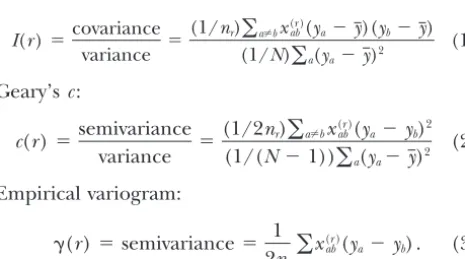
Moran’sI:
which approaches zero for large sample sizesN(Sokal
andWartenberg1983;Epperson2003).
I(r)⫽covariance
variance ⫽
(1/nr)
兺
a⬆bx(r)ab(ya⫺y)(yb⫺y)(1/N)
兺
a(ya⫺y)2(1)
Variogram modeling:The autocorrelation structure can be modeled by fitting a theoretical variogram model to
Geary’sc:
the empirical variogram. The elementary theoretical variograms suitable for modeling patterns due to a
sin-c(r)⫽semivariance
variance ⫽
(1/2nr)
兺
a⬆bxab(r)(ya⫺ yb)2(1/(N⫺ 1))
兺
a(ya⫺y)2(2)
gle, stationary spatial process are defined by the follow-ing parameters: (i) model family, such as exponential, Empirical variogram:
spherical, or Gaussian; (ii)nugget variance,i.e., the
vari-ance among adjacent samples; (iii)range, or the distance
␥(r)⫽semivariance⫽ 1
2nra⬆b
兺
x(r)ab(ya⫺ yb) . (3)
beyond which observations are spatially independent;
and (iv)sill, the constant variance among spatially
un-correlated samples (Figure 1A;IsaaksandSrivastava
GivenNsamples, these coefficients are calculated on
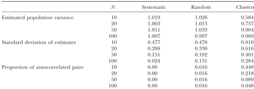
TABLE 1
Accuracy and precision of estimates of the population variance for different sampling designs
N Systematic Random Clustered
Estimated population variance 10 1.019 1.026 0.584
20 1.003 1.013 0.757
50 1.011 1.033 0.904
100 1.007 0.997 0.969
Standard deviation of estimates 10 0.477 0.478 0.810
20 0.288 0.330 0.616
50 0.151 0.192 0.401
100 0.024 0.131 0.284
Proportion of autocorrelated pairs 10 0.00 0.016 0.448
20 0.00 0.016 0.218
50 0.00 0.016 0.089
100 0.00 0.016 0.048
The autocorrelated data were generated by dividing an ordered vector of 500 random values from a standard normal distribution into groups of five consecutive values. The entire groups and the values within each group were reordered at random, representing a hypothetical transect where always five neighboring locations would show very similar values, with random steps between groups. The data set has an expected variance of 1.0 and the proportion of (autocorrelated) within-group comparisons is 0.016. Three types of samples were taken from the transect: (i) a random sample from all locations, (ii) a systematic sample selecting every fifth location, and (iii) a clustered sample, where entire groups of five neighboring locations were selected at random. Data simulation and sampling were repeated 1000 times for each sample size of 10, 20, 50, or 100.
Sensitivity of measures of autocorrelation and popu- (N ⫺ 1), assumes independent, spatially uncorrelated observations, which would correspond to a strictly hori-lation variance:Sensitivity to nonstationarity:The
assump-tion of weak staassump-tionarity can be violated in several ways, zontal empirical variogram. In essence, this requires
the assumption of a panmictic population with random including (i) nonstationarity of the mean in the
popula-tion,e.g., in the presence of clinal structure, (ii) nonsta- dispersal, which is likely to be violated in most natural
systems.
tionarity of the variance,e.g., if the variability of a
micro-satellite locus increases with increasing number of repeats, Spatial autocorrelation reduces the variance between
closely spaced pairs of observations. The following simu-or (iii) anisotropy, where the autocsimu-orrelation structure
depends on direction, e.g., if mean seed dispersal dis- lation illustrates the consequences of spatial
autocorre-lation for estimating the popuautocorre-lation variance and thus tances are larger than average in the predominant wind
direction. Strictly speaking, the stationarity assumption for rescaling Moran’sIand Geary’sccorrelograms. An
artificial, autocorrelated variable was sampled in differ-concerns the underlying process and not the observed
pattern, so that it cannot be tested directly (Fortinet ent ways and the estimates of the population variance,
averaged over many replicate simulations, were
com-al.2003). However, the empirical variogram can be used
to check for problems with nonstationarity. A finite, pared to the true value. We compared three sampling
strategies: (i) systematic sampling, with a spacing known constant variance will always result in the presence of
a sill, whereas a continued increase of the semivariance to be larger than the range of spatial autocorrelation
to obtain spatially uncorrelated, independent sampling with distance may indicate a spatial trend in the mean,
possibly coupled with dependence of the variance on the units; (ii) random sampling; and (iii) stratified or
clus-tered sampling, selecting groups of nearby locations to mean. Separate empirical variograms can be calculated
for different directions and compared to check for an- obtain an appropriate representation of short distance
classes for spatial analysis. The criteria for comparison isotropy. In theory, the same visual inspections could
be performed with correlograms, but only the variogram wereaccuracy,i.e., the absence of bias so that the mean
of all replicate estimates is close to the true population offers the possibility of modeling different components
of variance and, thus, accounting for them. For instance, value, andprecision,i.e., low variability of replicate
esti-mates (Palmer1990). For details of the simulation
ex-an exponential variogram function could be used to
model the autocorrelation due to a stationary spatial periment, see the Table 1 legend.
The systematic and the random samples provided process, and a linear variogram function could be used
to model the increase in variance with distance due to unbiased estimates, independent of sample size (Table
1). Precision increased with sample size;i.e., the
stan-a cline.
Sensitivity to the sampling design:The variogram can be dard deviation of the estimates was reduced. For small sample sizes, where the chances of randomly selecting interpreted as a distance-dependent estimate of the
popu-lation variance (Wagner2003). The commonly used “un- autocorrelated samples were small, the systematic and
the random samples reached a similar precision. With
increasing sample size, however, the random samples be estimated from pairwise comparisons, so that vario-grams can be defined that provide an estimate of genetic provided a lower precision than the systematic samples.
diversity as a function of geographic distance. This effect was due to the increasing number of
compar-Variogram of molecular variance:The univariate defini-isons between autocorrelated samples, not their
propor-tion of a variogram (Equapropor-tion 3) can be extended to tion. Parametric statistical tests assume spatially
uncorre-multivariate data. Thus, under the SMM,yaandyb are
lated samples, which in this simulation corresponds to
not two observations of the allele sizeylof a single locus
the systematic sampling design. For a spatially
autocor-l, but vectorsYaandYbof two observations of the
num-related variable, the increased variability of estimates
ber of repeats atLloci. The empirical semivariance␥ˆ(r)
from a random sample may render such tests too liberal.
becomes half the squared Euclidean distance betweenYa
This means that the actual probability of rejecting the
andYband is equal to the sum of the empirical
semivari-null hypothesis when it is true (type I error) may be
ances␥ˆl(r) of the number of repeatsyl(Wagner2003):
larger than the stated significance level␣.
On average, the clustered samples strongly
underesti-␥ˆ(r)⫽ 1 2nra⬍
兺
b兺
L
l⫽1 x(r)
ab(yla⫺ylb)2
mated the population variance (Table 1). This negative bias was reduced with increasing sample size, as more
and more clusters of samples were selected, thus reduc- ⫽ 1
nra
兺
⬍b兺
Ll⫽1 x(r)
ab␥ˆl(a,b)⫽
兺
l␥ˆl(r) . (4)
ing the proportion of comparisons between autocorrel-ated pairs of samples. In fact, the variance of the
esti-More generally, a multivariate variogram can be defined mates based on clustered samples was comparable to
as a weighted average␥(r) of the component variograms
the variance for systematic samples with a five times ␥
ˆl(r), with Equation 4 as the special case ofwl⫽1:
smaller sample size, which can be explained by the
sam-pling of clusters of five strongly autocorrelated loca- ␥(r)⫽
兺
l
wl␥ˆl(r) . (5)
tions. However, the clustered samples provided biased
Most often, the variograms of theLloci will be weighted
estimates, whereas the corresponding systematic
sam-bywl⫽ 1/L.
ples were unbiased. Hence, the unbiased variance
esti-Under SMM, genetic diversity is related to differences mator may be negatively biased due to spatial
autocorre-in allele size, where allele sizeylais defined as the number
lation. The magnitude of this systematic bias will depend
of repeats of gene copyaat locusl. The molecular variance
on the spatial autocorrelation structure and the
propor-of a single locuslwithkalleles can be defined as
tion of autocorrelated samples, which are functions of the spatial configuration of the sample rather than
sam-Vˆl⫽ N N⫺1
兺
kplk(ylk⫺ yl)2⫽
1
N⫺1
兺
a(yla⫺yl)2
ple size. One may argue that the spatial autocorrelation structure is an inherent characteristic of a population.
(Renwicket al.2001), where
However, because the estimate of the population vari-ance depends on the sampling design, it should be
yl⫽
兺
kplkylk ⫽
1
N
兺
ayla. (6)
based on independent samples.
Correlograms imply division by the sample or
popula-tion variance (see Equapopula-tions 1 and 2). Because of this, Equations 4 and 6 provide a distance-dependent
esti-it follows that (i) the actual values of Moran’sI(r) and mateVˆ(r) of the molecular varianceVˆ, averaged over
Geary’sc(r) depend on the spatial configuration of the Lloci, which can be used as a within-population analog
toRSTto investigate isolation-by-distance effects within
sample, and (ii), for a stationary process,I(r) reaches
a continuous population:
a value slightly below zero, andc(r) a value above one,
for distances beyond the range of spatial
autocorrela-Vˆ(r)⫽
兺
a⬍b
兺
Ll⫽1 wlx(r)ab
2nr
(yla⫺ylb)2. (7)
tion. The exact deviation cannot be predicted without knowing the spatial autocorrelation structure and the
details of the sampling design. This is not accounted The statistical significance of a departure ofVˆ(r) from
for by subtractingE[I(r)]⫽ ⫺1/(N ⫺ 1) for Moran’s its expected value under the null hypothesis of no spatial
I(r). On the other hand, an empirical variogram can autocorrelation can be tested in a Mantel permutation
test (LegendreandLegendre1998). If the alternative
be used to estimate the real population variance
ac-hypothesis is positive spatial autocorrelation at short counting for autocorrelation, usually by fitting a
theoret-distances, a one-sided test with a progressive Bonferroni ical variogram model. Hence, the above exemplified
correction can be applied, where the significance level
problem of Moran’sIand Geary’sccan be avoided.
for the kth distance class is ␣/k(Hewitt et al.1997;
LegendreandLegendre1998;Lichsteinet al.2002).
This correction is appropriate when significant
autocor-DEVELOPMENT OF METHODS
relation is hypothesized to occur in the smallest distance Definition of genetic variograms:This paragraph shows classes and the aim is to determine the extent of spatial
structure (Legendre andLegendre 1998).
Variogram of gene diversity: The analysis of the genetic dates different ploidy levels or multiple sampling of
structure of a locus lunder the IAM is often based on genets. If the different gene copies of the same diploid
join-count statistics. The proportion of unlike joins be- or polyploid organism are not assumed to be
indepen-tween observations is equivalent to the sum of the vario- dent,e.g., due to inbreeding, one may want to restrict
grams of a set of dummy variables zk, where zka ⫽ 1 if comparisons to gene copies from different individuals.
gene copyais of allele k, andzka⫽0 otherwise: In organisms with various ploidy levels, one may want
to give equal weight to each individual independent of ␥ˆl(r)⫽
兺
ka
兺
⬍b x(r)ab
2nr
(zl ka⫺zlkb)2. (8) its ploidy level. Both problems can be solved by
modi-fying the weightsx(r)
ab,
Due to the inherent correlation between the dummy
variables,␥ˆl(ab) will equal 1 if gene copiesa andb are
x⬘(r) ab ⫽
冦
x(r) ab
1
Ni
1
Nj
, i⬆j
0, i⫽j,
different alleles and 0 if they are the same allele.
Gene diversity or expected heterozygosity of a locus (13)
is a key parameter in population genetics under IAM.
Gene diversityHlis the probability that two gene copies whereNiis the number of gene copies of individualiwith
sampled with replacement differ at locus l. The unbi- gene copy a and Nj is the number of gene copies of
ased estimator of gene diversity, Hˆl, at locus l for a individualjwith gene copyb. The same type of weighting
sample ofNgene copies ofkdifferent alleles is can be applied to account for multiple sampling of genets
in clonal organisms. In that case,Niis the number of gene
Hˆl⫽ N
N ⫺1
冢
1⫺兺
k p2k
冣
(9) copies from geneti, etc.The permutation test needs to be adapted so that,
in-(Nei1978). stead of permuting gene copies, the individuals or
geno-On the basis of Equations 8 and 9, the variogram of types are permuted.
multilocus gene diversityHˆ can be defined as Modeling of genetic variograms:Expected shape of
spa-tial genetic structure: Theoretical models of
isolation-Hˆ(r)⫽
兺
L
l⫽1
wl␥ˆl(r)⫽
兺
a⬍b兺
L
l⫽1
兺
k wlx(rab)2nr
(zlka⫺zlkb)2. (10) by-distance predict that, in a two-dimensional space and
if certain conditions are met, kinship or relationship
co-Hˆ(r) provides a within-population analog toFST. As efficients between individuals, as well as pairwise FST or
with Vˆ(r), the significance of an observed autocorrela- RST, vary approximately linearly with the logarithm of
dis-tion inHˆ(r) can be tested with a Mantel permutation tance (Rousset1997;HardyandVekemans1999;Hardy
test. 2003). Thus, with some assumptions concerning the
Variogram of genotypic diversity:Genotypic diversity mea- drift-dispersal-mutation equilibrium and the dispersal
sured by Simpson’s diversityDis similar to single-locus function, the observed spatial genetic structure can be
gene diversityHˆl, but, instead of allelek, the multilocus quantified to infer gene dispersal parameters
(Veke-genotypegis used, so thatDis the probability of sam- mansandHardy2004). The general approach, as
de-pling two individuals of different multilocus genotypes. scribed byVekemansandHardy(2004), is to estimate
The unbiased estimator of genotypic diversity is the probability of identity in state as a function of the
spatial distance between individuals. Because this
func-Dˆ ⫽ N
N⫺1
冢
1⫺兺
g p2g
冣
. (11) tion depends on the variability and thus the mutation rateof the locus, it needs to be standardized, for instance, by
The variogram of genotypic diversityDˆ (Simpson di- reference to random genes from a sample of individuals
versity) is obtained by coding each multilocus genotype (Rousset 2000, 2002). The standardized valuesF(r) for
by a dummy variablezg, which takes the valuezg⫽1 if each distance classrare regressed against spatial distance
individualais of genotypegandzg⫽0 if it is not. For (one-dimensional case with linear relationship) or against
a haploid organism, the analysis is based on gene copies, the logarithm of distance (two-dimensional case with
expo-whereas for diploid organisms, genotype coding would nential relationship) to estimate the slope parameterbˆ
F.
normally reflect diploid genotypes. The variogram of
AsbˆFis negative and depends somewhat on the sampling
genotypic diversity, Dˆ(r), estimates the probability of
design,VekemansandHardy(2004) proposed
quanti-sampling two individuals of different multilocus
geno-fying spatial genetic structure by a new statistic, Sp ⫽
types as a function of their distance in space and is
bˆF/(1⫺ FN), where FN is the relatedness of immediate
calculated as
neighbors competing for the same resources and may
be estimated byF(1), the value ofF(r) for the first distance
Dˆ(r)⫽
兺
a⬍b
兺
g x(r)ab
2nr
(zga⫺ zgb)2. (12)
class. If the observed, two-dimensional spatial genetic structure results solely from isotropic limited gene dis-persal, if a dispersal-drift equilibrium has been reached, Accounting for ploidy levels and clonality:This
distance of the organism, then dispersal parameters can landscapes, such as wooded pastures and chestnut
or-be estimated from Sp (VekemansandHardy2004). chards (Scheideggeret al.2002).
Exponential variogram model:Assuming an exponential re- Data: We studied the spatial genetic structure of a
lationship in a two-dimensional case (see above), the spatial continuous population ofL. pulmonariafrom the Swiss
genetic structure of a population can be summarized by Jura Mountains. A hierarchical random sample of 461
fitting an exponential variogram model (Figure 1), thalli was collected from a pasture-woodland landscape.
In a first step, 100 circular plots of 1 ha were randomly ␥(r)⫽C0⫹ C1[1⫺e⫺(3r/b)] , (14)
selected from the wooded parts of the study area. Within
whereC0 is the nugget variance, or the proportion of each plot, all suitable trees exceeding 5 cm in diameter
the variance that is not spatially structured, andC1 is at breast height were searched forL. pulmonaria. A
maxi-the spatially structured variance component (Legendre mum of 24 thalli were randomly selected from different
andLegendre1998). The sillC⫽C0⫹C1provides an trees in each of the 24 plots where the lichen was
pres-estimate of the population variance based on spatially ent. If there were⬍24 colonized trees, multiple thalli
independent samples,i.e., accounting for spatial auto- were sampled from the same tree, and if there were
correlation. The relative size of the nugget provides an ⬍24 thalli in a plot, every thallus found was included.
estimate ofFN: 1⫺C0/C⫽C1/C⫽FˆN. This can be set This results in a heterogeneous data set that could
ex-toF(1)by fitting a fixed-nugget model, constraining the hibit spatial autocorrelation at varying scales.
nugget variance to the observed semivariance for the DNA extraction and fragment length determination
first distance class. at six microsatellite loci (LPu03,LPu09,LPu15,LPu16a,
The exponential model approaches the sillCasymp- LPu20a, and LPu27a), specific to the haploid
mycobi-totically. Therefore, the range or slope parameterbindi- ont, using an ABI 3100-Avant automated sequencer
(Ap-cates the practical range of the exponential variogram, plied Biosystems, Foster City, CA), followed Walseret
i.e., the distance at which the curve reaches 95% of the al.(2003). Allele assignment was performed using
GE-sill (JournelandHuijbregts 1978). It can be shown NOTYPER 2.5 software (Applied Biosystems).
thatb⫽ ⫺3/bˆF. Directional dispersal or migration may Statistical analyses: Omni-directional variograms of
lead to anisotropy, where the genetic structure depends molecular varianceVˆ(r) and gene diversityHˆ(r) were
on direction. If there is reason to expect anisotropy, direc- calculated according to Equations 7 and 10, giving equal
tional variograms can be fitted, providing estimates of the weight to each of the six loci. The first distance class of
slope parameterbfor different compass directions. r⫽0 contained pairs of thalli from the same tree. The
A confidence interval for the slope parameterbmay lag distance was 50 m. The last distance class contained
be estimated using the permutation method for the all sample comparisons at distances⬎450 m.
Autocorre-confidence interval for the matrix regression coefficient lation was tested per distance class using a one-sided
proposed byManly(1997). The residuals of the expo- Mantel test with 500 permutations of the thalli and a
nential model are randomly permuted many times to progressive Bonferroni correction of␣ ⫽0.05/kfor the
obtain the reference distribution of the correlation of kth distance class up to the first nonsignificant value.
the residuals with distance. A series of exponential mod- A second set of variograms,Vˆ⬘(r) andHˆ⬘(r), was
calcu-els with varying range parameters is derived, and the lated weighting each thallus by the number of
occur-critical values are determined at which the correlation rences of its multilocus genotype within the population,
of the residuals of these new models with distance is as using modified weightsx⬘(r)
ab (Equation 13).
Autocorrela-strong as for the␣/2 and the (1 ⫺ ␣)/2 quantiles of tion was again tested per distance class using a one-sided
the reference distribution. The two critical values pro- Mantel test with 500 permutations of the multilocus
vide the lower and upper limits of the confidence inter- genotypes, using the same settings as above.
val for the range parameterb. An isotropic and four-directional variograms of
geno-typic diversity Dˆ(r) were also calculated according to
Equation 12, giving equal weight to all samples.
Expo-APPLICATION TO THE GENETIC STRUCTURE
nential variogram models were fitted to all variograms,
OFL. PULMONARIA
using the weighted least-squares algorithm (Cressie Model organism: L. pulmonariais a foliose epiphytic 1993) that minimizes the expression
lichen species of humid temperate and boreal regions of the northern hemisphere and cooler parts of the
兺
rnr冢
␥ˆ(r) ␥(r;C0,C1,b)
冣
2
, (15)
tropics (Yoshimura 1971). This clonal and
recombi-nant species (Walseret al.2004), which produces both
where␥(r;C0,C1, b) is the fitted semivariance for
dis-vegetative and sexual diaspores, is considered
endan-tance classron the basis of the exponential model with
gered in most parts of Central Europe (Wirth et al.
parametersC0,C1, andb.
1996) and in other industrialized regions. It is used as
All calculations were performed in R (Ihakaand
Gen-an indicator of ecological continuity (Rose 1992) in
persal (Table 2). On the other hand, genotypic diversity showed a higher degree of autocorrelation for the first
distance class,Fˆ(1), which consisted of pairs of samples
from the same tree. The fitting of directional variograms for genotypic diversity revealed that spatial genetic struc-ture extended further in the main wind direction
(WSW–ENE;Vittoz1998) than in the other directions
(Table 2).
The conventional estimates of the population
vari-ance,Vˆ,Hˆ, andDˆ, slightly underestimated the variance
for spatially independent samples, i.e., the total sill C
for all three measures of diversity (Table 2). In this specific example, however, weighting for recurrent ge-notypes largely compensated this bias.
Figure2.—Variogram of gene diversityHˆ(r) for a popula-tion of Lobaria pulmonaria. Each symbol denotes the mean
DISCUSSION semivariance over six microsatellite loci averaged over all pairs
of thalli within each distance class. The semivariance is
un-Advantages of variogram analysis:A geostatistical
per-weighted (circles) or per-weighted for recurrent genotypes (squares).
spective on spatial genetic structure can provide
expla-The lines indicate the corresponding fitted exponential
mod-nations to many of the issues raised byVekemansand
els; the dashed line shows the nonspatial model. Values below
the dashed line correspond to positive, and values above the Hardy(2004) and suggest new approaches to address
dashed line to negative, autocorrelation. Solid symbols indi- them. First, the sampling design has a strong influence cate statistically significant positive autocorrelation based on
on the absolute values of Moran’sIor other coefficients
a one-sided Mantel permutation test with progressive
Bonfer-of relatedness, and this may severely limit comparability
roni correction (␣ ⫽0.05).
between studies. The sampling design also affects the distance at which these measures reach their expected value in the absence of spatial structuring. Therefore, this distance provides only a somewhat arbitrary
esti-using the R library “GSTAT” (PebesmaandWesseling
1998;Pebesma2004). mate of the extent of spatial genetic structure
(Veke-mansandHardy2004). This problem affects the
analy-Results and discussion:On the basis of the six
micro-satellite markers, we found 92 multilocus genotypes of sis of kinship structure with Moran’sI or relationship
coefficients, where empirical values for larger distances
the haploid mycobiont of L. pulmonaria. All but 9
multilocus genotypes occurred in single 1-ha plots, and tend to be slightly below zero, whereas in theory negative
kinship coefficients are not allowed (Barbujani1987).
only 1 was spread over ⬎210 m. The probability of
origin by recombination was ⬍0.003 for all recurrent Our simulation experiment showed that this effect is
not simply due to sample size, but relates to the inclusion multilocus genotypes, suggesting that they arose from
clonal propagation. Weighting for recurrent genotypes of autocorrelated samples in the estimation of the
popu-lation variance, which is commonly used as a reference drastically reduced effective sample size from 461 thalli to
92 multilocus genotypes. For recurrent genotypes, pairwise for rescaling correlograms and other measures of
relat-edness. Variogram modeling, on the other hand, pro-comparisons were distributed over several distance classes:
the first distance class contained an equivalent of 36.8 vides an estimate of the population variance accounting
for spatial autocorrelation, and its model parameters pairs (instead of 1588 for all samples) and the other
distance classes up to 450 m comprised 47.6–148.6 pairs are scaled by this corrected estimate.
Second,VekemansandHardy(2004) suggested that
(instead of⬎2000).
The spatial genetic structure of the studiedL. pulmo- if a plot of F(r) against distance r, e.g., a Moran’s I
correlogram, decreases steadily until some distance x
naria population consisted of two patterns caused by
clonal reproduction [variogram of genotypic diversity, and shows no further trend, this distance may be
inter-preted as the extent of spatial genetic structure. In
geo-Dˆ(r)] and sexual reproduction [variograms of
molecu-lar variance,Vˆ(r), and gene diversity,Hˆ(r); Figure 2]. statistical terms, this means that if the variogram
repre-sents a stationary spatial process as indicated by the Weighting for recurrent genotypes reduced the
autocor-relation of the first distance class and the range estimate presence of a sill, the rangebcan be estimated. Rather
than visually identifying a critical distance at which the both for molecular variance and for gene diversity
(Ta-ble 2). After weighting for clones, the range parameters sill is reached, one would fit an exponential variogram
model and estimate the practical range, where the curve
b of the fitted exponential variogram models were
smaller for molecular variance,Vˆ⬘(r), and gene diversity, reaches 95% of the sill. This provides an estimate of the
extent of spatial genetic structure. A confidence interval
Hˆ⬘(r), than for genotypic diversity, Dˆ(r), suggesting
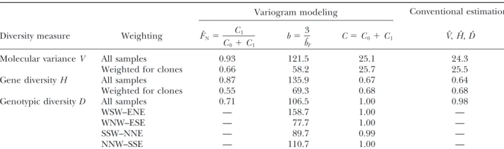
TABLE 2
Variogram parameters forLobaria pulmonaria
Variogram modeling Conventional estimation:
Diversity measure Weighting FˆN⫽
C1 C0⫹C1
b⫽ 3 bˆF
C⫽C0⫹C1 Vˆ,Hˆ,Dˆ
Molecular varianceV All samples 0.93 121.5 25.1 24.3
Weighted for clones 0.66 58.2 25.7 25.5
Gene diversityH All samples 0.87 135.9 0.67 0.64
Weighted for clones 0.55 69.3 0.68 0.68
Genotypic diversityD All samples 0.71 106.5 1.00 0.98
WSW–ENE — 158.7 1.00 —
WNW–ESE — 77.7 1.00 —
SSW–NNE — 89.7 0.99 —
NNW–SSE — 110.7 1.00 —
Estimated parameters of the exponential variogram model were fitted to the variograms of molecular variance and gene diversity for a population ofLobaria pulmonaria(N⫽461) assessed with six microsatellite markers, with and without accounting for recurrent genotypes, and for genotypic diversity (clonal structure), with and without accounting for compass direction. The relatedness between immediate neighbors,FN, is estimated from the autocorrelation of the first distance class of thalli taken from the same tree. The range parameterbdenotes the distance at which the curve reaches 95% of the sill and provides an estimate of the extent of spatial genetic structure. The total sillCestimates the population diversity (molecular variance, gene diversity, or genotypic diversity) accounting for spatial autocorrelation, whereas the conventional estimatorsVˆ,Hˆ, andDˆ do not account for autocorrelation and are, therefore, susceptible to bias.
method developed for matrix regression coefficients by links. This method is related to thecc-correlogram
pro-posed by Bertorelle and Barbujani (1995), which
Manly(1997).
Third, the interpretation of Moran’sIas a correlation involves division by the population variance, and could
easily be adapted to dominant markers such as randomly coefficient or of other measures as the absolute degree
of kinship or relationship is jeopardized by the depen- amplified polymorphic DNA (RAPD), intersimple
se-quence repeat (ISSR), or amplified fragment length dence of the empirical values on the sampling design
through an implicit rescaling (see above). The proposed polymorphism (AFLP) markers.
Fourth,VekemansandHardy(2004) proposed a new
empirical variograms, however, have direct interpretations
independent of the sampling design, as they provide dis- statistic for quantifying spatial genetic structure, Sp⫽ ⫺bF/
FN, which arguably is more robust than either of the two
tance-dependent estimates of molecular varianceVˆ, gene
diversityHˆ, and genotypic diversity Dˆ, providing within- component measures that are sensitive to the sampling
design (see above). Rather than taking the ratio of two
population analogs to the population pairwiseRSTandFST
statistics. potentially biased quantities, variogram modeling
ac-counts for the source of this potential bias by estimating
The variogram of molecular variance,Vˆ(r), for
micro-satellite data has a straightforward interpretation as the the variance between uncorrelated samples. Hence, the
variogram parameters nugget variance, range, and sill variance in the number of repeats expected for samples
at a given distance in geographic space. It corresponds can be directly compared between studies.
Further-more,FNcan be estimated in two different ways. If the
directly to a plot of (half) the sum of squared size
differ-ences as used in AMOVA of microsatellite data (Schnei- first distance class contains the direct neighboring
sam-ples, thus representing the smallest possible distance, der et al. 2000) or of D0/2, where D0 is the average
squared difference in repeat numbers for two alleles the semivariance for this distance class can be used as
an estimate ofFN(fixed nugget-effect model).
Alterna-drawn from the same population (Goldsteinet al.1995).
The variogram of genotypic diversity,Dˆ(r), can be inter- tively, if the first distance class also contains not directly
adjacent samples, the nugget effect needs to be fitted, preted as the probability of sampling two different
multilocus genotypes as a function of their spatial dis- providing an estimate ofFN.
Robust estimation of spatial genetic structure:Weighting
tance. The interpretation of the variogram of gene
diver-sity, Hˆ(r), is the probability of sampling two different for clonality and ploidy levels:The lichen example illustrated
the importance of distinguishing between spatial patterns alleles given their distance in geographic space,
aver-aged over different loci. For a single locus, it corre- of clonality and of genetic diversity resulting from sexual
recombination. Specifically, it is crucial to account for sponds exactly to a plot of the proportion of unlike
links against distance, but the variogram definition is clonal patterns when analyzing patterns of genetic
not represent the average of the two component pat- in situations with at least 50% nugget variance (Cressie
terns, but their multiplication, so that the degree and 1993). We will perform simulations to assess to what
extent of spatial genetic structure may be severely over- degree robust variogram estimators may help reducing
estimated. sample size within populations.
For diploid organisms, the weighting results in mea- Conclusions:Most measures of spatial genetic structure
sures similar to the kinship coefficient by Loiselle et are rescaled with reference to random samples from the
al.(1995) and the relationship coefficient ofStreiffet population. This reference is itself estimated from the data
al.(1998), as links within individuals are excluded. The set and subject to bias unless spatial autocorrelation is
weighting proposed here is more general and can accounted for. Such bias limits the interpretation of
abso-equally be used for organisms with variable ploidy levels lute values of various measures of spatial genetic structure
and applied to the correlation coefficientrbySmouse and poses problems to the comparison between studies
andPeakall(1999) or to join-count statistics (Epper- and to the estimation of biological parameters (Vekemans
son2003). The proposed weighting of clones solves the and Hardy2004). Variogram modeling, on the other
problem of arbitrary resampling of recurrent genotypes, hand, estimates its reference value accounting for
spa-which may bias the analysis of spatial genetic structure tial autocorrelation, thus providing parameter estimates
within continuous populations (Reuschet al.1999;Ha¨m- that are comparable between studies. Furthermore, the
merliandReusch2003). Whether to weight for recur- proposed variograms of molecular variance, gene
diver-rent genotypes or not will depend on the research ques- sity, and genetic diversity are directly interpretable
with-tion (e.g., dispersal distancesvs.distances between mates) out rescaling, as they provide a partitioning of genetic
and the type of organism under study (e.g., clonal organ- diversity by the distance between samples. While this
ar-isms with physically connected or detached ramets). ticle focuses on microsatellite data as interpreted under
Deviation from exponential relationship: Simulations either IAM or SMM, the approach may be adapted to
showed that under isolation-by-distance on a two-dimen- other types of genetic data. The formal integration with
sional grid, Moran’sItypically drops from positive values variograms makes the theory and tools of geostatistics
at short distances to negative values at intermediate available for population genetics, which may help to
distances before reaching values just below zero for address some important challenges in bridging the gap
larger distances in the absence of a cline (Epperson between empirical studies of spatial genetic structure
2003). In our L. pulmonaria example, the variograms and theoretical approaches to isolation-by-distance.
of molecular variance (not shown) and gene diversity
We thank Magnus Nordborg and two anonymous reviewers for their
showed evidence for such a humped distribution. This
helpful comments on this and an earlier version of the manuscript.
type of nonmonotonic autocorrelation structure is often This research is part of a project funded by the Swiss National Science
encountered in geostatistical analysis and may arise Foundation under the National Centre of Competence in Research
(NCCR) Plant Survival and through grant 3100A0-105830/1.
from a periodic structure (PyrczandDeutsch2003)
or as a sampling artifact (Journel and Huijbregts
1978; Palmer and White 1994). It may be modeled
LITERATURE CITED
by a dampened sine hole-effect model (Journeland
Balloux, F., andJ. Goudet, 2002 Statistical properties of
popula-Huijbregts1978;LegendreandLegendre1998). In
tion differentiation estimators under stepwise mutation in a finite
addition, a clinal structure may cause a linear change island model. Mol. Ecol.11:771–783.
of variance with distance, which can be modeled by a Balloux, F., andN. Lugon-Moulin, 2002 The estimation of
popula-tion differentiapopula-tion with microsatellite markers. Mol. Ecol.11: linear variogram model. Anisotropic variograms can
155–165.
help identify clinal structure,e.g., in the case of
direc-Balloux, F., L. LehmannandT. de Meeus, 2003 The population
tional dispersal. genetics of clonal and partially clonal diploids. Genetics164:
1635–1644.
Robust variogram estimation:Testing of differences
be-Barbujani, G., 1987 Autocorrelation of gene frequencies under
tween spatial patterns from different populations is
no-isolation by distance. Genetics117:777–782.
toriously difficult, as the hypothesis concerns the under- Bertorelle, G., andG. Barbujani, 1995 Analysis of DNA diversity
lying process and not its observed realization (Fortin by spatial autocorrelation. Genetics140:811–819.
Burrough, P. A., 1995 Spatial aspects of ecological data, pp. 213–
et al.2003). Many measures of spatial genetic structure
251 inData Analysis in Community and Landscape Ecology, edited
suffer from a high sampling variance (Vekemans and by R. H. G.Jongman, C. J. F. ter Braak and O. F. R. van
Hardy2004). Thus, rigorous statistical testing requires Tongeren. Cambridge University Press, Cambridge, UK.
Cavalli-Sforza, L. L., 1984 Isolation by distance, pp. 229–248 in
a large number of replicate populations, each with a
Human Population Genetics: The Pittsburgh Symposium, edited by
large internal sample. Several robust variogram estima- A.Chakravarti. Van Nostrand Reinhold, New York.
tors exist (CressieandHawkins1980;Cressie1993). Chung, M. G., andB. K. Epperson, 2000 Clonal and spatial genetic
structure inEurya emarginata(Theaceae). Heredity84:170–177.
WhileCavalli-Sforza(1984) used a robust variogram
Cliff, A. D., andJ. K. Ord, 1981 Spatial Processes: Models and
Applica-estimator based on the median variance, the modulus
tions. Pion, London.
variogram(CressieandHawkins1980) has been shown Cressie, N. A. C., 1993 Statistics for Spatial Data. John Wiley & Sons,
New York.
Cressie, N., andD. M. Hawkins, 1980 Robust estimation of the Pebesma, E., andC. G. Wesseling, 1998 Gstat, a program for geo-variogram. J. Int. Assoc. Math. Geol.12:115–125. statistical modelling, prediction and simulation. Comput. Geosci.
Epperson, B. K., 2003 Geographical Genetics. Princeton University 24:17–31.
Press, Princeton, NJ. Piazza, A., andP. Menozzi, 1983 Geographic variation in human
Fenster, C. B., X. VekemansandO. J. Hardy, 2003 Quantifying gene frequencies, pp. 444–450 inNumerical Taxonomy, edited by gene flow from spatial genetic structure data in a metapopulation J.Felsenstein. Springer, Berlin.
of Chamaecrista fasciculata (Leguminosae). Evolution 57: 995– Pyrcz, M., and C. Deutsch, 2003 The whole story on the hole 1007. effect. Newsl. Geostat. Assoc. Australas.18:3–5.
Fortin, M.-J., M. R. T. Daleand J.ver Hoef, 2001 Spatial analysis Renwick, A., L. Davison, H. Spratt, J. P. KingandM. Kimmel, 2001 in ecology, pp. 2051–2058 inThe Encyclopedia of Environmetrics, DNA dinucleotide evolution in humans: fitting theory to facts. edited by A. H.El-Shaarawiand W. W.Piegorsch. John Wiley & Genetics159:737–747.
Sons, Chichester, UK. Reusch, T. B. H., W. Hukriede, W. T. StamandJ. L. Olsen, 1999
Fortin, M. J., B. Boots, F. CsillagandT. K. Remmel, 2003 On Differentiating between clonal growth and limited gene flow us-the role of spatial stochastic models in understanding landscape ing spatial autocorrelation of microsatellites. Heredity83:120– indices in ecology. Oikos102:203–212. 126.
Goldstein, D. B., A. R. Linares, L. L. Cavalli-SforzaandM. W. Rose, F., 1992 Temperate forest management: its effects on bryo-Feldman, 1995 An evaluation of genetic distances for use with phyte and lichen floras and habitats, pp. 211–233 inBryophytes microsatellite loci. Genetics139:463–471. and Lichens in a Changing Environment, edited by J. W.Batesand
Goldstein, D. B., G. W. Roemer, D. A. Smith, D. E. Reich, A. A.Farmer. Clarendon Press, Oxford.
Bergmanet al., 1999 The use of microsatellite variation to infer Rousset, F., 1997 Genetic differentiation and estimation of gene population structure and demographic history in a natural model flow fromF-statistics under isolation by distance. Genetics145: system. Genetics151:797–801.
1219–1228.
Ha¨mmerli, A., andT. B. H. Reusch, 2003 Genetic neighbourhood Rousset, F., 2000 Genetic differentiation between individuals. J. of clone structures in eelgrass meadows quantified by spatial
Evol. Biol.13:58–62. autocorrelation of microsatellite markers. Heredity91:448–455.
Rousset, F., 2002 Inbreeding and relatedness coefficients: What do
Hardy, O. J., 2003 Estimation of pairwise relatedness between
indi-they measure? Heredity88:371–380. viduals and characterization of isolation-by-distance processes
us-Scheidegger, C., P. Clerc, M. Dietrich, M. Frei, U. Groneret
ing dominant genetic markers. Mol. Ecol.12:1577–1588.
al., 2002 Rote Liste der gefa¨hrdeten Arten der Schweiz: Baum-und Hardy, O. J., and X. Vekemans, 1999 Isolation by distance in a
Erdbewohnende Flechten. BUWAL, Bern, Switzerland. continuous population: reconciliation between spatial
autocorre-Schneider, S., D. RoessliandL. Excoffier, 2000 ARLEQUIN
Ver-lation analysis and popuVer-lation genetics models. Heredity83:145–
sion 2.000 : A Software for Population Genetic Data Analysis. Genetics 154.
and Biometry Laboratory, University of Geneva, Geneva.
Hardy, O. J., andX. Vekemans, 2002 SPAGEDi: a versatile computer
Slatkin, M., 1995 A measure of population subdivision based on program to analyse spatial genetic structure at the individual or
microsatellite allele frequencies. Genetics139:457–462. population levels. Mol. Ecol. Notes2:618–620.
Smouse, P. E., andR. Peakall, 1999 Spatial autocorrelation analysis
Hewitt, J. E., P. Legendre, B. H. McArdle, S. F. Thrush, C.
of individual multiallele and multilocus genetic structure.
Hered-Bellehumeur et al., 1997 Identifying relationships between
ity82:561–573. adult and juvenile bivalves at different spatial scales. J. Exp. Mar.
Sokal, R. R., andD. E. Wartenberg, 1983 A test of spatial autocorre-Biol. Ecol.216:77–98.
lation analysis using an isolation-by-distance model. Genetics105:
Ihaka, R., andR. Gentleman, 1996 R: a language for data analysis
219–237. and graphics. J. Comp. Graph. Stat.5:299–314.
Streiff, R., T. Labbe, R. Bacilieri, H. Steinkellner, J. Glo¨ sslet Isaaks, E. H., andR. M. Srivastava, 1989 Applied Geostatistics.
Ox-al., 1998 Within-population genetic structure inQuercus robur
ford University Press, New York.
L. andQuercus petraea(Matt.) Liebl. assessed with isozymes and
Journel, A. G., and C. J. Huijbregts, 1978 Mining Geostatistics.
microsatellites. Mol. Ecol.7:317–328. Academic Press, New York.
Legendre, P., and L. Legendre, 1998 Numerical Ecology. Elsevier, Van der Hulst, R. G. M., T. H. M. Mes, M. Falque, P. Stam, J. C. M.
Amsterdam. Den Nijset al., 2003 Genetic structure of a population sample of
Lichstein, J. W., T. R. Simons, S. A. ShrinerandK. E. Franzreb, apomictic dandelions. Heredity90:326–335.
2002 Spatial autocorrelation and autoregressive models in ecol- Vekemans, X., andO. J. Hardy, 2004 New insights from fine-scale ogy. Ecol. Monogr.72:445–463. spatial genetic structure analyses in plant populations. Mol. Ecol.
Loiselle, B. A., V. L. Sork, J. NasonandC. Graham, 1995 Spatial 13:921–935.
genetic structure of a tropical understory shrub,Psychotria offici- Vittoz, P., 1998 Flore et ve´ge´tation du Parc jurassien vaudois: typo-nalis(Rubiaceae). Am. J. Bot.82:1420–1425. logie, e´cologie et dynamiqu des milieux. Ph.D. Thesis, Universite´
Manly, B. F. J., 1997 Randomization, Bootstrap and Monte Carlo Methods de Lausanne, Lausanne, Switzerland.
in Biology. Chapman & Hall, London. Wagner, H. H., 2003 Spatial covariance in plant communities:
inte-Meirmans, P. G., E. C. Vlot, J. C. M. Den NijsandS. B. J. Menken, grating ordination, geostatistics, and variance testing. Ecology 2003 Spatial ecological and genetic structure of a mixed
popula-84:1045–1057. tion of sexual diploid and apomictic triploid dandelions. J. Evol.
Wagner, H. H., 2004 Direct multiscale ordination with canonical Biol.16:343–352.
correspondence analysis. Ecology85:342–351.
Monestiez, P., andM. Goulard, 1997 Analysing spatial genetic
Walser, J. C., C. Sperisen, M. SolivaandC. Scheidegger, 2003 structures by multivariate geostatistics: study of wild populations
Fungus-specific microsatellite primers of lichens: application for of perennial ryegrass (Lolium perenne), pp. 1197–1208 in
Geostatis-the assessment of genetic variation on different spatial scales in
tics Wollongong ‘96, edited by E. Y.Baafiand N. A.Schofield.
Lobaria pulmonaria.Fungal Genet. Biol.40:72–82. Kluwer, Dordrecht, The Netherlands.
Walser, J. C., F. Gugerli, R. Holderegger, D. KuonenandC. Nei, M., 1978 Estimation of average heterozygosity and genetic
dis-Scheidegger, 2004 Recombination and clonal propagation in tance from a small number of individuals. Genetics89:583–590.
different populations of the lichenLobaria pulmonaria.Heredity
Palmer, M. W., 1990 The estimation of species richness by
extrapola-93:322–329. tion. Ecology71:1195–1198.
Wirth, V., H. Scho¨ ller, P. Scholz, G. Ernst, T. Feuereret al.,
Palmer, M. W., andP. S. White, 1994 Scale dependence and the
species-area relationship. Am. Nat.144:717–740. 1996 Rote Liste der Flechten (Lichenes) der Bundesrepublik
Parks, J. C., andC. R. Werth, 1993 A study of spatial features Deutschland. Schriftenreihe fu¨ r Vegetationskunde28:307–368. of clones in a population of bracken fern,Pteridium aquilinum Yoshimura, I., 1971 The genusLobariaof Eastern Asia. J. Hattori (Dennstaedtiaceae). Am. J. Bot.80:537–544. Bot. Lab.34:231–364.
Pebesma, E. J., 2004 Multivariable geostatistics in S: the gstat
APPENDIX: WORKED EXAMPLE
Example data:The example data set consists of two artificial variablesy1andy2that describe the fragment lengths
x of two loci in N ⫽ 6 haploid individuals A–F along a transect t. There are three multilocus genotypes g with
differing frequencies:
t y1 y2 g
A 1 1 4 1
B 2 1 4 1
C 2 2 4 2
D 3 2 1 3
E 3 2 1 3
F 4 2 1 3
Spatial partitioning of molecular variance:The basic elements of spatial covariance are calculated as
␥ˆl(a,b)⫽
1
2(yla⫺ylb)
2.
For instance, the comparison of gene copyAto gene copiesBandDprovides
␥ˆ(A,B)⫽ 1 2
兺
i(yiA⫺yiB)2⫽
1
2((1⫺ 1)
2⫹ (4⫺4)2)⫽ 0
␥ˆ(A,D)⫽ 1 2
兺
i(yiA⫺yiD)2⫽
1
2((1⫺2)
2 ⫹(4⫺ 1)2)⫽5 .
The semivariance␥ˆi(a,b) for each pair of gene copies is tabulated in the following matrix:
␥ˆ(a,b) A B C D E F A ⫺ 0 0.5 5 5 5
B 0 ⫺ 0.5 5 5 5
C 0.5 0.5 ⫺ 4.5 4.5 4.5
D 5 5 4.5 ⫺ 0 0
E 5 5 4.5 0 ⫺ 0
F 5 5 4.5 0 0 ⫺
Matrix of distances r:Common geostatistical analysis omits distances ofr⫽0, so that an object is never compared
to itself. For organisms such as the epiphytic lichen L. pulmonaria, however, individuals may share the same
two-dimensional geographic coordinates if they grow on the same tree. Therefore, it may be important to distinguish between different individuals separated by a distance of zero in two-dimensional space and the comparison of an individual with itself:
r A B C D E F
A ⫺ 1 1 2 2 3
B 1 ⫺ 0 1 1 2
C 1 0 ⫺ 1 1 2
D 2 1 1 ⫺ 0 1
E 2 1 1 0 ⫺ 1
F 3 2 2 1 1 ⫺
Variogram of molecular variance:The empirical variogram of molecular variance is calculated using Equation 7, as
is illustrated here for distance classr⫽2 on the basis of unique pairs only [top or bottom triangle of matrices␥(a,