New Techniques for Functional Data Analysis: Model Selection, Classification, and Nonparametric Regression.

(1)

ABSTRACT

AVERY, MATTHEW ROGERS. New Techniques for Functional Data Analysis: Model Selection, Classification, and Nonparametric Regression. (Under the direction of Hao Helen Zhang and Yichao Wu.)

Functional data, such as curves and images, are increasingly collected in many research

dis-ciplines due to rapid advances in computers and modern scientific technologies. Compared to

traditional scalar- or vector-data, functional data are inherently infinite-dimensional and more

complex, and the observations from random trajectories are often sparse and irregularly

sam-pled. In such cases, traditional statistical methods can not be directly applied, and new methods

must be developed. Here, we study three problems related the functional data.

First, we look at the problem of sparse regression for functional data. In traditional settings,

sparse regression refers to model selection problems where a subset of ap×1vector of predictor variables is chosen to model the response. In functional data, we consider a model with a scalar

response, Y and associated functional predictorX(t) observed over some domain T. In this context, a sparse model is one in which the coefficient functionβ(t)forX(t)is set identically to 0over some subset of T. Rather than choose a subset of predictor variables, we choose a subset of the domain of a single functional predictor. We propose a method for sparse regression

using the Fused LASSO with a 1st order b-spline basis. This two-stage method is flexible and

can be used in conjunction with all methods for functional regression.

Next, we consider the problem of classification for functional data, which has important and

broad applications in practice. A new discriminant analysis approach is developed and studied.

(2)

(FPCA) and then conduct linear discriminant analysis (LDA) based on the FPCA scores.

Com-pared with existing functional data classification methods, the new procedure is conceptually

much simpler, easier and faster to implement, and competitive in performance. The demanded

programming effort is minimal, as the procedure can take advantages of existing software

pack-ages. Theoretical justifications are provided for the procedure in terms of its classification

con-sistency under certain conditions.

Finally, we consider nonlinear functional regression for sparse and irregular data. As in the

traditional setting, most methods for functional regression impose specific model assumptions

on the data. If the true relationship between predictor and response does not conform to these

assumptions, the resulting estimates may be poor. We propose a nonlinear regression method

for functional data. Unlike other nonparametric methods discussed in the literature, ours can be

applied to sparse and irregularly sampled data because it uses PACE to estimate the predictor

trajectories. We compare our method to existing parametric methods on simulated data as well

(3)

(4)

New Techniques for Functional Data Analysis: Model Selection, Classification, and Nonparametric Regression

by

Matthew Rogers Avery

A dissertation submitted to the Graduate Faculty of North Carolina State University

in partial fulfillment of the requirements for the Degree of

Doctor of Philosophy

Statistics

Raleigh, North Carolina

2012

APPROVED BY:

Daowen Zhang Ana-Maria Staicu

Hao Helen Zhang

Co-chair of Advisory Committee

Yichao Wu

(5)

BIOGRAPHY

Matthew Avery was born in Davis, CA to Joy and Michael Avery. He grew up in Gainesville,

FL, graduating from Eastside High School with an IB Diploma in 2002. He received his

Bach-elor of Arts Degree in Economics from New College of Florida in 2006 after completing his

dissertation,The Welfare Effects of Direct to Consumer Advertising in Prescription Drug

Mar-kets. He began studying statistics at NCSU in 2006, and now moves on to pursue a career at

(6)

ACKNOWLEDGEMENTS

It has taken the efforts of many people for me to reach this point, and here I give an incomplete

list. My family, Mom, Dad, and Lily, have constantly cheered for me and pushed me forward. I

wouldn’t be here without them. I got some great help as an undergraduate, particularly from my

adviser, Dr. Richard Coe, as well as Dr. Catherine Elliott. I’m not sure anyone has done more to

spur my interest in learning and academics than Dr. Elliott. There’s no way I would’ve gotten

through graduate school without the encouragement and support of my friends and classmates,

Justin, Paul, Malorie, Laura, David, Adam, Frank and Carrie. Special thanks to Kat for her

notes and suggestions. Finally, this dissertation would not have come together without my

advisers, Dr. Helen Zhang and Dr. Yichao Wu, who’ve given me good direction at every turn.

(7)

LIST OF TABLES

Table 2.1 Simulation results for all methods withβ(t)Unimodal,n= 50,p= 35 . 40 Table 2.2 Simulation results unimodal coefficient function for different values of

nwith EBIC tuning. (p= 35) . . . 43

Table 2.3 Simulation results for Z coefficient function for different values of n with EBIC tuning. (p= 35) Note: Trimmed means reported. . . 44

Table 2.4 Simulation results for bimodal coefficient function for different values ofnwith EBIC tuning. (p= 35) . . . 45

Table 2.5 Error rates for Unimodal coefficient with measurement error . . . 46

Table 2.6 Error rates for Z coefficient function with measurement error . . . 47

Table 3.1 Classification errors for Case 1 (computation time in minutes) . . . 66

Table 3.2 Classification errors for Case 2 (computation time in minutes) . . . 68

Table 3.3 Classification errors 3-class simulation (computation times in minutes) . 70 Table 3.4 Classification errors for 4-class simulation (computation times in minutes) 71 Table 3.5 Classification errors for 5-class simulation (computation time in minutes) 72 Table 3.6 Classification errors for “real world” data sets . . . 74

Table B.1 Simulation results for triangle coefficient function for different values of nwith EBIC tuning. (p= 35) . . . 99

Table B.2 Simulation results for Valley coefficient function for different values of nwith EBIC tuning. (p= 35) . . . 100

(10)

LIST OF FIGURES

Figure 1.1 Three types of functional data . . . 9

Figure 1.2 Gene expression data before and after smoothing with PACE . . . 16

Figure 2.1 Canadian Weather Data . . . 21

Figure 2.2 Two sets of basis functions . . . 24

Figure 2.3 Initial and second stage stage fits . . . 30

Figure 2.4 Submanifold . . . 37

Figure 2.5 Example curves . . . 38

Figure 2.6 Sparse fits for different coefficient functions . . . 41

Figure 2.7 Sparse fits for different coefficient functions . . . 42

Figure 3.1 Example curves from gene expression and spinal bone mineral density data sets . . . 50

Figure 3.2 Case 1 mean functions and simulated data points . . . 65

Figure 3.3 Case 2 mean functions and simulated data points . . . 67

Figure 3.4 Multiclass mean functions and simulated data points . . . 73

Figure 3.5 Gene expression data: Raw data, estimated FPC curves, and smoothed estimates of data . . . 75

Figure 4.1 Boxplots of average squared prediction errors. The top row is the reg-ular case, and the bottom row is the sparse case. The first column uses modelF1 and the second column uses modelF2. . . 90

(11)

Chapter 1 Introduction

As technology progresses and more and more data becomes available, statistical methods must

keep up. In particular, new data types, such as images and functions, come with new challenges.

Functional MRIs produce images that neuroscientists and psychologists would like to use to

learn about psychological diseases and neural connectivity. Data that might previously have

been treated as longitudinal is now being treated as functional data. In such situations, new

methods must be devised that leverage the unique characteristics of the data.

For standard data, common problems include model selection, classification, and

nonparamet-ric regression. Model selection techniques are employed in a variety of cases, such as when

one is unsure which predictors are (most) important for modeling the response. These methods

choose a subset of predictors, resulting in a sparse model that is generally easier to interpret

than the full model. We frame the model selection problem as choosing a subset of the

do-main of a functional predictor rather than a subset of different predictors. By identifying such

(12)

Also, interpreting the predictor’s relationship with the response may be simpler, since it will

be defined only over a certain range.

For standard data, k-class classification is well-studied, but this problem also arises when the

predictors are curves. Particularly when the observed data are sparsely and irregularly sampled,

simple methods for classification are desirable. Similarly, while linear and quadratic regression

have been proposed for functional data, both methods rely on a specified parametric model.

When the data does not conform to this model (as in the case of a complex nonlinear

relation-ship), the resulting estimators may not be consistent. A more general approach, particularly in

the case of sparse and irregularly sampled data, may be able to model such relationships more

accurately.

1.1 Regression

The standard linear regression model fornobservations andppredictors can be written as

y=Xβ+, (1.1)

whereyis a vector ofnresponse variables,X is ann×pdesign matrix whoseith row,xT_i = [xi1, xi2], . . . , xip, consists of the values of the p predictor variables for the ith observation,

β is a vector of coefficients for the p predictors, and is an n×1 vector of random errors. When necessary, we will assumeX has been normalized and the responses centered. That is, Pn

(13)

From this general framework, many methods have been developed for estimating the

coeffi-cients, β. The simplest method is to chooseβ to minimize the residual sum of squares. That

is, minimize

||y− p X

j=1

xjβj||2. (1.2)

This is commonly known as Ordinary Least Squares (OLS) regression.

1.1.1 Penalization Methods

While OLS works well in simple cases, it may not always be appropriate. For example, whenp is large, the model may be difficult to interpret as well as over-fit. A common approach in such

cases is penalized regression, where rather than minimize 1.2, we minimize

||y− p X

j=1

xjβj||

2₊_P

λ(β), (1.3)

where Pλ(β) is a penalization function with parameter λ whose argument is the coefficient vector. Common examples of penalty functions include the Ridge Regression penalty (Hoerl

and Kennard, 1970), which is the L2 _{norm of the coefficient vector, and the LASSO (Least}

(14)

||y− p X

j=1

xjβj||

2₊_λ||_β_||.

(1.4)

These penalization methods yield coefficient estimates that have simpler interpretations than

the standard OLS fit. For example, when a regression problem has many predictor variables

(that is, p is large), many of the estimated coefficients may be small. Small marginal effects can be difficult to interpret, since while they may be “statistically significant”, they may not be

significant in a practical sense. The LASSO addresses this issue by setting these small marginal

effects to be exactly zero. The resulting fit is simpler to interpret than the OLS fit. Indeed, the

LASSO is performing variable selection, since relatively few predictors are “selected” to be

in the estimated model. The resulting model is called “sparse”, since many predictor variables

have been weeded out, and we are left with a smaller “sparser” model.

Since the LASSO was first described, numerous methods have been devised using this

penal-ized regression framework. The Adaptive LASSO (Huang et al., 2006) uses weights from, for

example, the standard OLS fit to scale the penalty applied to each predictor coefficient. The

Adaptive LASSO also enjoys the Oracle property, which the standard LASSO does not. The

Elastic Net (Zou and Hastie, 2005) is useful for selecting groups of highly correlated variables.

While the standard LASSO will typically select only one of these predictors and exclude the

rest, the Elastic Net is designed to include the whole group in the estimated model.

Finally, the Fused LASSO (Tibshirani et al., 2005) finds sparse fits for models where

con-secutive predictors may be included in the model. This is done by penalizing the differences

between consecutive coefficients in addition to penalizing the coefficients directly. For this

ap-proach, we must presuppose that the predictor variables conform to an underlying structure

(15)

predicting the response,y, then we believe the(j −1)th and(j+ 1)th variables may also be important. This occurs when the predictor variables have some relevant ordering to them, such

as the case when the predictors represent observations at consecutive time points. Alternatively,

the ordering can be constructed by placing correlated predictors near one another. (Tibshirani

et al., 2005) To fit the Fused LASSO, we minimize

||y− p X

j=1

xjβj||

2

+λ1||β||+λ2||βdif f||, (1.5)

whereβ_{dif f} = (β2−β1, β3−β2, . . . , βp −βp−1)andλ1, λ2are penalization parameters. The

resulting fits are characterized by large ranges of consecutive coefficients set identically to 0.

The Fused LASSO has applications for functional data which will be explored in Chapter 2.

1.1.2 Nonparametric Regression

The previous discussion has focused on the subset of regression models where a particular

relationship between the predictors and the response is assumed prior to model fitting. While

this has the advantage of producing good model estimates when the true relationship is

consis-tent with the model assumptions, when these assumptions are violated, the resulting estimates

may be biased. One solution to this is nonparametric regression. In this approach, the only

assumption is that

(16)

Once again,xi is a vector of predictor variables foryi, and i is the random error for the ith observation. To estimateµ(·), a common approach is kernel regression. LetK(·)be a suitable (non-negative, symmetric, withR K(t)dt = 1) kernel andhnbe an associated bandwidth. Then a nonparametric estimator fory∗ with associated predictor vectorx∗is

Pn

i=1YiK(x ∗₋_x

i

hn )

Pn i=1K(

x∗₋_x

i

hn )

. (1.7)

This is the multivariate version of the Nadaraja-Watson estimator. See also Fan and Gijbels

(1996). The choice of bandwidth and kernel function are important, and have been discussed

in Rice (1984) and Fan and Gijbels (1992).

1.2 Functional Data

In both genetics and biostatistics, multiple observations on a single subject over time are

in-creasingly being treated as realizations from a single underlying process. This so-called

func-tional data has motivated numerous new techniques that leverage its unique characteristics to

fit more accurate models. A general overview of functional data analysis including some

fun-damental methods was given by Ramsay and Silverman (2005).

Generally, a functional variable can be defined as a smooth process that occurs over some

domain, typically time. When modeling functional data, both response variables as well as

predictors can be functional, though we focus here on the case of a scalar response with an

(17)

Ideally, we would want to observe the functional variable over its entire domain. This is the

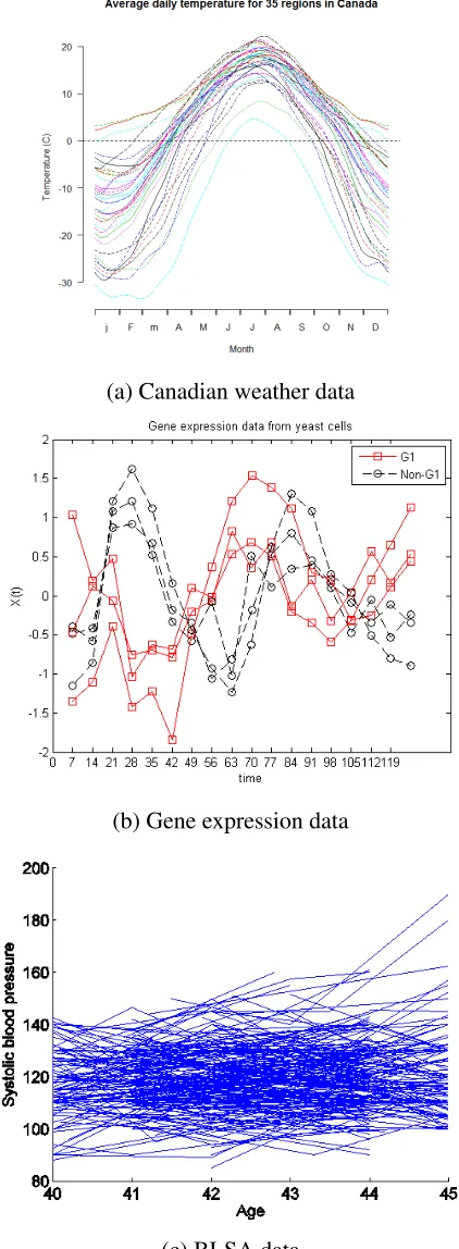
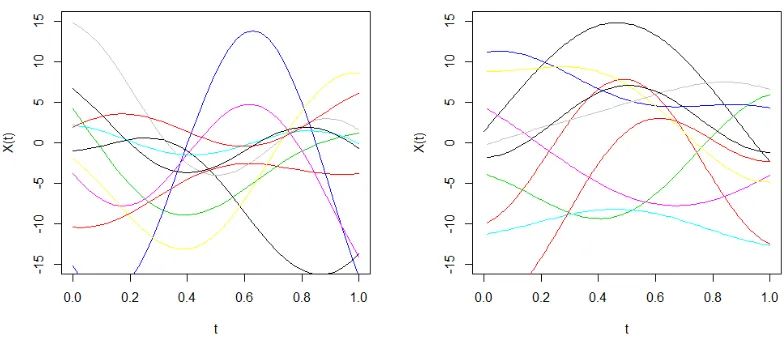
case with Canadian weather data discussed in Ramsay and Silverman (2005). For each of 35

regions, average daily temperatures are recorded, giving us a temperature trajectory over the

course of a full year. In this case, the trajectories are said to be regularly observed on a dense

grid of time points. These curves are given in Figure 1.1a.

The Canadian weather data is an ideal situation where the grid of observed points is sufficiently

dense that the underlying process can easily be interpolated. It is more common to observe

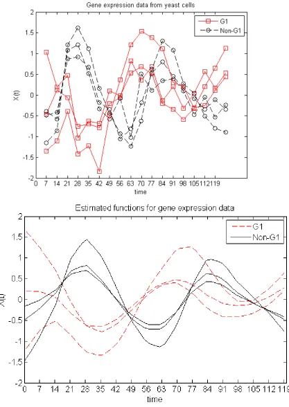
fewer points for each trajectory. For example, Spellman et al. (1998) look at temporal gene

expression data from yeast cells. (See Figure 1.1b.) In this case, for each gene, the expression

level is observed at a total of 18 time points over the course of roughly 2 hours. Once again,

the grid of observed points is fixed, but unlike the Canadian weather data, there are many fewer

observations. In this case, the underlying process must be estimated through some process,

such as smoothing splines.

In the case of longitudinal data, even less information may be available. Particularly when the

subjects involved are people, it may not be possible to observe the subject at regular intervals,

and some times, subjects may only be observed as few as one or two times. Data of this type is

referred to as sparse, irregularly sampled data, since times at which observations are made are

not fixed and the number of observations for some subjects may be very few. This is typical of

longitudinal studies such as the Baltimore Longitudinal Study of Aging, where values such as

blood pressure were measured on subjects when they visited the Gerontology Research Center.

(Shock et al., 1984) Since subjects would drop out of the study or miss appointments, not

all individual trajectories were frequently observed or observed over the full time frame of

the study. Similarly, Bachrach et al. (1999) observed spinal bone mineral densities for males

(18)

many of the subjects only a few observations were made. (In some cases, as few as one or two

observations were recorded.) From Figure 1.1c, we can see that these data look quite different

from the previous examples.

1.2.1 Regression for functional data

Consider the functional linear regression model

Yi =β0+

Z

T

Xi(t)β(t)dt+i, i= 1, . . . , n. (1.8)

Here, the scalar response, Yi is modeled using a functional predictor variable,Xi(t), defined over some domain, T ∈ _R. Often times for simplicity, T will be scaled to [0,1]. The rela-tionship betweenyiandXi(t)is determined by the coefficient function,β(t), andi is random error. We assume that the predictor curves,Xi(t)and the coefficient function,β(t)are square-integrable functions onT.

1.2.2 Notation for functional data

Typically, the full curve,Xi(t)is not observed. Rather, for the ith curve, we observeX(t)at some numberNi >0of discrete time points,Ti1, ..., TiNiordered such thatTij < Ti(j+1), where

(19)

(a) Canadian weather data

(b) Gene expression data

(20)

studies, e.g. Rhein and Strimmer (2006) and Spellman et al. (1998)) or it may be randomly

determined (e.g.James and Hastie (2001), Bachrach et al. (1999), Rice and Wu (2001)).

Additionally, we assume these observations are made with some measurement error, denoted

δij. Let the observed value for theith curve at timeTij beUij =Xi(Tij)+δij. The measurement errors are assumed be independent both between and within curves with mean0andvar(δij)< ∞. Our regression model requires the full curve,Xi(t)to findYi. Thus, we must estimate the full curve using the available data before performing functional regression.

It is useful then to think of functional data as being one of two types. For the case where we have

fixed time points, the straightforward approach of using a local smoother over the observed

time points can be employed provided the grid of observations is sufficiently dense. (Ramsay

and Silverman, 2005) Other approaches are necessary when the data is sparsely sampled at

irregular time points. One such method is Principal component Analysis through Conditional

Expectation or PACE, (Yao et al., 2005b) which can be applied to irregularly sampled data with

very few observations per time point. The resulting estimated principal component functions

and scores can be used to estimate the underlying curves,Xi(t). We will discuss PACE further in the next section.

Once we have estimated the predictor curves, we perform regression and estimate the

coeffi-cient function. If we restrictβ(t)to the space of smooth functions with no further assumptions, identifiability is an insurmountable problem. One approach to dealing with this is to perform

regression with a smoothness penalty. That is, we chooseβb(t)to minimize

X

Yi− Z

T

Xi(t)βb(t)dt

+λ

Z

T

b

(21)

whereβ(d)₍_t₎_{is the} _{dth derivative of} _β₍_t₎ _and_λ _{is a penalty term. Thus, the estimated}

func-tion is chosen to have smooth dth derivative. A more common method is to assume that the coefficient function can be decomposed using some orthogonal basis such that the first p basis functions can well-approximate β(t). Then we write β(t) = B(t)T_η_{, where} _B₍_t_{) =}

[b1(t), b2(t), . . . , bp(t)]T, and η is a vector of coefficients. Thus, the regression problem be-comes

Yi =β0+xTi η+i, (1.10)

wherexij = R

T Xi(t)bj(t)dt. We can now find estimates forηusing any number of traditional

methods, such as OLS described above. When we employ this basis decomposition approach,

the choice of orthogonal basis,B(t)is of paramount importance. If we use PACE to estimate the curves, the principal component basis makes the most sense. In this case, the FPC scores

become the design matrix,X.

1.2.3 Functional Principal Components

Functional Principal Components (FPC) is a useful method for analyzing functional data.

Recall that for standard data, principal components is a nonparametric method used for

ex-ploratory data analysis and dimension reduction. For the regression model defined in Eq. 1.2,

letX be a normalized design matrix. Then(XT_X₎−1 _{is the corresponding scaled covariance}

matrix. We can find the principal components by calculating the eigenvectors fromXTX. Note that these eigenvectors will be mutually orthogonal and form a complete basis for the vector

(22)

that solves

argmax

x

ggT_l (XTX)g_l, s.t. g_lTg_l = 1andgT_lg_m = 0∀m < l. (1.11)

That is, thelth principal component will be the unit vector in the direction of maximal variation forXT_X _{that is orthogonal to the first}_l₋₁_{eigenvectors.}

Once we have found the eigenvectors, we can calculate the principal component scores for

each observation by finding linear combination of the eigenvectors that returns its original

co-efficients. For each eigenvector, there is an associated eigenvalue,λl, which corresponds to the variability ofXexplained by the eigenvalue. It is standard to order the eigenvectors/eigenvalues such thatλ1 ≥ λ2 ≥ . . . ≥ λp. The dimension of the problem can be reduced by choosing a subset of eigenvectors, l = 1, . . . , K such thatPK_l₌₁λl is sufficiently close to

Pp

l=1λl. The reduced model is then

y=XDβ∗+, (1.12)

whereXD _{is the matrix of the first}_K _{principal component scores for each observation, and}_β∗

is the coefficient vector for the eigenvectors.

Functional principal components can be defined through analogy to the standard principal

com-ponents method described above. Under the functional regression model given in Eq. 1.8, the

(23)

argmax

φl(t)

Z

T

Z

T

φl(s)V(s, t)φl(t)dsdt s.t. Z

T

φl(t)φl(t)dt= 1, Z

T

φl(t)φm(t)dt= 0∀m < l. (1.13)

Then, the lth eigenfunction is the normalized function that captures the most variability from V(s, t) and is orthogonal to all previous eigenfunctions. Unlike in the traditional principal components case, this is not a finite basis, and l = 1,2, . . .. Typically, this expansion is trun-cated afterK eigenfunctions such thatPK_l₌₁λl is sufficiently close to P

∞

l=1λl, where thelth

eigenvalue,λlis defined as

λl = Z

T

Z

T

φl(s)V(s, t)φk(t)dsdt. (1.14)

We can write our data using the Karhunen-Lo`eve representation and the FPC basis as

Xi(t) =µ(t) +

∞

X l=1

ξilφl(t), (1.15)

whereµ(t)is the mean function of {Xi(t)}ni=1,ξil is the lth FPC score for theith curve, and V ar(ξ_l) =λl.

1.2.4 FPC for Sparse and Irregularly Sampled Data

Many examples are given in the literature for finding the eigenfunctions, eigenvalues, and FPC

(24)

these methods are focused on the case when the predictor curves are sampled over a dense grid.

When data is sparsely sampled at irregular intervals, finding consistent estimators for the FPC

scores can be challenging. Principal components Analysis through Conditional Expectation

(PACE, Yao et al. (2005b)) offers a way to find these estimates when some curves are observed

as few as one or two times.

Suppose instead of observing the predictor curves on a dense grid they are observed sparsely

and irregularly, as in the case of the BLSA data from Figure 1.1c. In this scenario, curveXi(t)is observed at time pointsTi1, ..., TiNiwith measurement errorδij, such that at timeTijwe observe

Uij =Xi(Tij) +δij. LetTi andUi denote the vectors of time points and observed values for theith curve respectively. Using local polynomial smoothers (see, for example, Fan and Gijbels (1996)), we can estimate the mean function for the data,µ(t)as well as the covariance surface, V(s, t). Consistent estimates for the lth FPC score for the ith curve conditional on the time points observed can be written as

˜

ξil =E(ξil|Ui,Ti) =λlφTilΣ

−1

Ui(Ui −µi). (1.16)

In this expression,ΣUi = V(Ti,Ti), φil = φl(Ti), and µi = µ(Ti)respectively. These are all estimated using the estimated version of these processes found earlier. Along with thelth estimated eigenvalue, we can plug in these estimates to find our estimator for the(i, l)th FPC score. The PACE estimate for theith curve is then

b

Xi(t) =µ_b(t) +

K X

l=1

b

(25)

whereK is chosen via some algorithm. (BIC is suggested by Yao et al. (2005b).) Figure 1.2 shows the gene expression data discussed above as well as the estimated curves using PACE.

1.2.5 Fitting Functional Regression Models

Once the true curves are estimated, the regression model must be fit. The functional linear

regression model (Yao et al. (2005a) and Ramsay and Dalzell (1991), for example) use the

model

E(Y|X) = β0 +

Z

T

β(t)XC(t)dt, (1.18)

whereXC₍_t_{) =}_X₍_t₎₋_µ

X(t)is the centered predictor function andβ(t)is the corresponding coefficient function. This coefficient function is analogous to the coefficient vector in a multiple

linear regression, where instead of a functional predictor we have a vector of predictor variables

associated with each response.

Much like linear regression in traditional settings, functional linear regression may be too

re-strictive to accurately model the relationship between the predictor and the response. Yao and

M¨uller (2010) introduced functional quadratic regression and general functional polynomial

regression which allow for more flexible fits. The functional quadratic regression model

as-sumes

E(Y|X) = β0+

Z

T

β1(t)XC(t)dt+

Z

T

Z

T

(26)

(27)

with similar extensions possible for higher-order terms. By including a quadratic term, this

model is capable of accurately modeling a larger set of relationships between the predictor and

response than linear regression.

The approach to estimation is similar for both of these models. First, an appropriate basis is

chosen. Yao et al. (2005a) and Yao and M¨uller (2010) use PACE to estimate the functional

principal component basis and corresponding FPC scores, but when full curves are observed,

other bases are viable. For estimablity, we truncate the chosen basis afterpbasis functions. De-note this truncated basis asB(t) = [b1(t), b2(t), . . . , bp(t), ...]T. Then the coefficient function can be approximated as β(t) = B(t)T_η_{, where}_η _{is a vector of coefficients. Thus, the linear} regression problem becomes

Yi =β0+xiη+i, (1.20)

wherexij = R

T Xi(t)bj(t)dt. We can estimateηusing any of the traditional methods described above, such as OLS.

The process is similar for functional quadratic regression, with

β2(x, t) =

p X m=1

m X

l=1

ηlmφl(s)φm(t)

(28)

1.3 Dissertation Outline

The remainder of this dissertation is organized in three main sections. Each section introduces

a new method for analysis of functional data. In Chapter 2, we discuss sparse functional linear

regression. The problem of interest is to identify regions on the domain, T of the functional predictor, X(t), such that ∀ t ∈ T0 _{⊂ T}_, _β₍_t_{) = 0}_{. We propose a two stage method that}

uses the Fused LASSO with a 1st order b-spline basis to identify these regions. This method

is flexible in that it can be applied after any method is used to find an initial (not necessarily

sparse) fit.

Chapter 3 addresses the problem of classification for functional data. There are examples in the

literature (including the spinal bone mineral density data discussed above) where curves come

from two or more classes. In such cases, identifying the differences between these classes and

being able to classify new curves is useful. We propose a method motivated by linear

discrim-inant analysis to address these issues. Our method is generally simpler in its application than

other methods, can be generalized to cases with three or more classes, and is computationally

efficient. Additionally, it can be applied to sparse and irregularly sampled data since it is based

on PACE.

Finally, Chapter 4 introduces a method for nonlinear functional regression. Functional linear

regression and functional quadratic regression have both been discussed in the literature, but

both methods rely on parametric models. If the relationship between the predictor and response

do not conform to the assumed model, these methods can produce poor results. Other

nonpara-metric models for functional data exist in the literature, but these assume that the predictor

curve is fully observed. Our method does not rely on parametric model assumptions, so it is

(29)

(30)

Chapter 2 Model Selection for Functional Data

2.1 Motivation

Model selection is an important area in traditional statistical analysis. Methods such as the

LASSO are used to choose models that simultaneously capture the relationship between the

response and covariates and ensure a sparse fit. These two characteristics are also desirable

when considering functional data, but the notion of “sparsity” may look somewhat different

in this setting. When multiple covariates are considered, analysis similar to the scalar case

may be appropriate, but for a single functional predictor, “sparsity” can viewed relative to the

domain of the covariate. A“sparse” model can be defined as one with a coefficient function,

β(t), that takes the value zero over a subset of the domain, T, of X(t). That is for some T0 _{⊂ T}_,_β₍_t_{) = 0}_∀t_{∈ T}0_{. Typically, we assume}_T0 _{consists of a small number of contiguous}

(31)

(a) Average daily temperatures at 35 different weather stations

(b) Estimated coefficient function for Cana-dian weather data

Figure 2.1: Canadian Weather Data

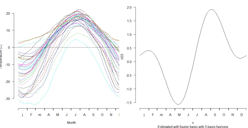
For example, consider the Canadian weather data discussed in Ramsay and Silverman (2005).

Average daily temperatures over nearly four decades are treated as predictors for annual rainfall

in 35 distinct regions in Canada. A plot of the predictor curves is given in Figure 2.1a. Using

standard functional regression techniques, we can estimate a coefficient function relating the

daily temperatures to the annual rainfall of a region. Figure 2.1b shows an estimate for β(t)

using functional linear regression with a fourier basis. This fit shows two major peaks (one in

the spring, the other in the fall) but does not identify any regions where there is no relationship

between average daily temperature and rainfall. A sparse fit would ideally retain as non-zero

the regions where the relationship between temperature and annual rainfall was strongest but

also identify other regions where the relationship may not be relevant.

(32)

functional regression and existing methods for sparse functional regression. Section 3

intro-duces our new method for sparse functional regression, and Section 4 discusses computational

issues. We demonstrate the effectiveness of this method through simulation in Section 5 and

show the performance of our method on the Canadian weather data set. Section 6 concludes

with a brief discussion.

2.2 Functional Regression

2.2.1 General Approach

A standard approach to functional regression is to assume that the coefficient function can

be decomposed using some orthogonal basis such that the first p basis functions can well-approximateβ(t). Then we writeβ(t) =B(t)T_η_{, where}_B₍_t_{) = [}_b

1(t), b2(t), . . . , bp(t)]T and

ηis a vector of coefficients. Thus, the regression problem becomes

Yi =β0+xiη+i, (2.1)

wherexij = R

T Xi(t)bj(t)dt. We can now estimateηusing any number of traditional methods,

such as OLS described above. When we employ this basis decomposition approach, the choice

of orthogonal basis,B(t)is of paramount importance.

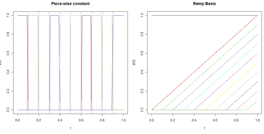
This is especially true for the problem of sparse regression, since our goal is to find a sparse fit.

(33)

functions should be included in the model (or equivalently, which should have their coefficients

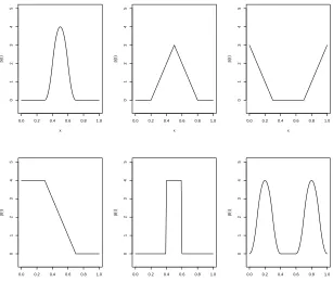
set equal to 0). B-splines are well-suited for this, since they are only defined on relatively small

intervals onT. For the simplest case, we can assume thatβ(t)is a step function and choose a 1st order b-spline basis to model it. Thus, we rewrite the regression function as

Yi = p X

j=1

βj Z

bj(t)X(t)dt, (2.2)

where

bj(t) = I(t∈Tj). (2.3)

Eachbj(t)takes nonzero values only on the regionTj whereTj = [t∗j−1, t∗j)forj = 1, . . . , p−1 andTp = [t∗p−1, t∗p]. While this basis may be used to find a sparse fit, step functions may not be flexible enough to accurately model the function. To fit more complex models, a linear fit may

be desired. The “ramp” basis may be useful for such cases. We define the “ramp” basis as

bj(t) = I(t∈[t∗j−1,1])∗(t−t

∗

j−1). (2.4)

Note that for the “ramp” basis, it is necessary to include an additional basis function,b0whose

(34)

(a) 1st order b-spline basis (b) Ramp basis

Figure 2.2: Two sets of basis functions

2.2.2 Existing Methods

Example of sparse functional regression are not prevalent in the literature. Functional Linear

Regression That’s Interpretable (FLiRTI, James et al. (2009)) was designed to find estimates of

coefficient functions that were easy to interpret. The authors proposed to find estimated

coeffi-cient functions that did not make large, rapid shifts. As such, they restrict certain derivatives of

the coefficient function to be sparse and estimate the restricted model using either the LASSO

or Dantzig selector. (Both approaches are endorsed by the authors.) The derivative on which the

restriction is placed can be thought of as a tuning parameter as well as a limit on the complexity

(35)

Lee and Park (2012) focus on limiting the number of basis functions included in the final

model rather than finding large regions onT that are necessarily zero. As such, they arrive at sparsity indirectly. By choosing a b-spline basis with a high initial number of basis functions

and then using any one of a variety of traditional variable selection techniques, they arrive at

an estimated coefficient function that is zero for a substantial portion of its domain. While this

method is novel in its assumption of a finite but unknown number of basis functions in the true

model, it does not require the included basis functions to adhere to any sort of pattern. This

could lead to fits that while sparse, may be difficult to interpret.

2.3 New Methods

For vector data, one of the most common methods for model selection is the least absolute

shrinkage and selection operator (LASSO, Tibshirani (1994)). The objective function for the

lasso is

Lλ1(y,X,η) = .5(y−Xη)

T₍_y₋_Xη_{) +}_λ

1

p X

j=1

|ηj|. (2.5)

Since for our case, a natural ordering exists for our coefficients (they correspond to basis

func-tions that represent consecutive subintervals on the domain ofX(t)), the fused lasso (Tibshirani et al., 2005), which penalizes adjacent terms for “jumps”, should also be considered. By

(36)

(a) 1st order b-spline fits using the Fused

LASSO (b) Ramp basis fits using the Fused LASSO

Lλ1,λ2(y,X,η) = .5(y−Xη)

T₍_y₋_Xη_{) +}_λ

1

p X

j=1

|ηj|+λ2

p X

j=2

|ηj−ηj−1|. (2.6)

The Fused LASSO takes advantage of the structure of the basis functions discussed above, all

of which have a natural ordering. For the 1st order b-spline basis, ifβi = 0thenβb(t) = 0for the subinterval associated withφi(t). Thus, by fusing together adjacent coefficients, we are forcing

b

β(t)to take constant values across subintervals of its domain. Since the lasso penalty tends to push individual coefficients towards 0, the result is large subintervals over which βb(t) = 0, giving us the sparse result we desire. Estimated coefficient functions fit using the fused LASSO

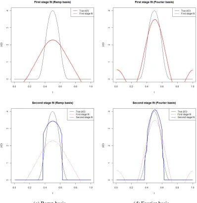
and 1st order b-spline basis on five simulated data sets are shown in Figure 2.3a.

Fits generated using the 1st order b-spline basis are not ideal. By construction, the fitted

tion must be a step function and will not be continuous. Moreover, if the true coefficient

(37)

A more flexible basis may be able to do a better job. In the case of the “ramp” basis, fusing

the coefficients results in a fit whose first derivative is constant over a subinterval. Estimated

fits from five simulated data sets are shown in Figure 2.3b. While this can make for an

easy-to-interpret function, it does not necessarily result in sparsity.

Full details for these fitting of these models is given in the Appendix.

2.3.1 Two-stage fitting

To find a model that will simultaneously be sparse while retaining the flexibility to estimate

complex functions, we take a two-stage approach. The first stage will give us an initial fit that

does a good job of modeling the function irrespective of sparsity. The second stage will alter

this initial fit to add sparsity.

The first stage is to estimate a coefficient function as accurately as possible using any method.

For example, first stage fit could be estimated using functional linear regression with the “ramp”

basis or a fourier basis. Define this estimate asβe(t). For this first step, we do not consider the sparsity of the fit, instead aiming to capture the shape of the true coefficient function. Using

e

β(t), we generate a new design matrix,X∗:

X∗_i,j =

Z

T

Xi(t)βe(t)b_j(t)dt, (2.7)

wherebj(t)is thejbasis function from the 1st order b-spline basis.

(38)

Lλ1,λ2(y,X

∗

, θ) =.5(y−X∗θ)T(y−X∗θ) +λ1

p X

j=1

|θj|+λ2

p X

j=2

|θj −θ(j−1)|. (2.8)

This is the fused lasso model from Eq. 2.6. We choose the penalty terms,λ1 andλ2via

cross-validation.

The second stage design matrix,X∗, incorporates the information from the first stage fit. If the coefficient function was estimated accurately, thenθ =1T should do a good job of minimizing Eq. 2.8. If there are regions onβ(t)that can be set to 0 without hurting prediction, the second stage should identify them, giving us a sparse fit. And if the first stage fit is not scaled correctly,

the second stage will modify it to give us a more accurate final result. The final 2-stage estimate

is computed by taking the point-wise product of the two estimated coefficient functions

b

β(t) =βe(t)∗θe(t), (2.9)

whereθe(t) = Pp

j=1θe_jφ_j(t), and the{φ_j(t)}is the 1st order b-spline basis.βb(t)will be set to exactly 0 over intervals where the second-stage selector has specified a region to be 0. By using

this two stage approach, we utilize the sparsity from the Fused LASSO and 1st order b-spline

basis while retaining the good fit from generated in the first stage. The result is that we have

the flexibility to model the coefficient function accurately while still ending up with a sparse

fit.

Also, note that this two stage technique can be applied to any first-stage fit estimate in order to

(39)

e

β(t)and then estimateθe(t). Examples of this method using the “ramp” basis to estimateβe(t) are given in Figure 2.3.

2.3.2 Sparsely Observed Trajectories and Measurement error

To this point, we haven’t addressed how to estimate the predictor trajectories, Xi(t). If the curves are fully observed, this is unnecessary. Consider the Canadian weather data. We observe

each trajectory 365 times, making this a close approximation of the ideal situation when the

full curve is observed. In many other applications, substantially less data may be available and

some consideration must be given for finding estimates,Xb(t)of the full curves.

When data is regularly observed on a relatively dense grid, it is possible to smooth each curve

individually. In this case, many options are available. Various scatter plot smoothing methods

(see Cleveland (1979) and Fan and Gijbels (1996) among others) as well as smoothing splines

(Green and Silverman, 1994) are available for this type of analysis. When the data is sparse

and irregularly sampled, estimating the individual curves can be more difficult. In such cases,

it may be better to estimate all of the curves simultaneously. Principal components Analysis

through Conditional Expectation (PACE, Yao et al. (2005b)) is one method for doing this. Once

the principal component functions and scores have been estimated, estimates for the individual

curves can be recovered.

Measurement error adds another level of complexity to the issue. Many of the issues associated

with measurement error for vector data are also relevant to functional data. Particularly, while

it may be possible to find unbiased estimates for each trajectory using smoothing splines as

(40)

(c) Ramp basis (d) Fourier basis

(41)

estimated with these curves,βb(t), will be biased. When the level of measurement error is very small, effect on the estimator may not be great, but with even modest levels of measurement

error, the estimated coefficient function will be poor. In these cases, a calibration step should

be used when estimating the predictor curves. Zhang et al. (2007) describe a nonparametric

calibration approach which could be used to estimate the predictor trajectories. PACE (Yao

et al., 2005b) is another possibility.

2.3.3 Summary of Algorithm

We summarize our method in three steps:

• Step 0: If necessary, find good estimates for the predictor curves,Xb_i(t).

• Step 1: Obtain a good estimate forβ(t). (This can be done using any method; sparsity it not a concern.) Denote this asβe(t)

• Step 2: CreateX∗ and estimate sparsity function,eθ(t).

(42)

2.4 Computational issues

2.4.1 Tuning for

λ

1

and

λ

2

The lasso and fused lasso penalties, λ1 and λ2 respectively, (denoted together as λ) must be

tuned appropriately to get a good fit. For standard penalized regression methods, many

cri-terion for tuning penalty terms exist. In early work, we considered four methods including

Akaike Information Criterion (AIC, Akaike (1974)), Bayesian Information Criterion (BIC,

Schwarz (1978)), Extended Bayesian Information Criterion (EBIC, Chen and Chen (2008)),

and cross-validation (CV). Each has its own unique objective function which we minimize to

find “optimal” values forλ. For cross-validation, we chooseλto minimize the cross-validation

squared prediction error. The squared prediction error for theith observation is

(Yi−Yb_iλ)2, (2.10)

whereYb_iλis the predicted response for theith curve for a given value ofλ. LetF₁, F₂, . . . , F_K be randomly selected sets such thatF1 ∪F2 ∪. . .∪FK = {1,2, . . . , n} andFk∩Fm = ∅, where1≤m6=k≤n. LetFC

k ={1,2, . . . , n}/Fkbe the compliment ofFk. Then for a given

λ, theK-fold cross-validation squared prediction error is

Errorλ=

K X k=1

X i∈Fk

(Yi−Yb_FλC

k,i

)2, (2.11)

whereYbλ FC

k,idenotes the predicted response for the

(43)

and the smoothing parameter,λ.

Alternatively, we can chooseλbased on any of a few popular tuning criteria. For example, for AIC, we chooseλto maximize

AIC =nlog(_bσ2) + 2df, (2.12)

whereσ_b2 = P

(Yi−Yb_i)2 anddf is the model degrees of freedom, defined as the number of unique values taken by theβbin the fused LASSO regression. Similarly, for BIC and EBIC, we have

BIC =nlog(_bσ2) +log(n)df, (2.13)

and

EBIC =nlog(_bσ2) + (log(n) +log(p))df. (2.14)

These two methods increase the penalty on using more degrees of freedom when the sample

size becomes large with the objective of preventing over-fitting. In the case of EBIC, models

that include larger numbers of basis functions are also penalized for overfitting. This criterion

was originally devised with genome-wide association studies in mind. In that situation,

overfit-ting can lead to high false discovery rates. This can be thought of as analogous to our situation,

(44)

To chooseλ, the relevant objective function is optimized using a Newton-related method in the

functionoptim with R (R Development Core Team, 2011). Based on early simulation results

not reported here, cross-validation, BIC, and EBIC are roughly equivalent, with each showing

marginally better performance in some situations. Optimization through cross-validation takes

substantially longer than the alternatives. For the results reported below, EBIC was used to tune

λ.

2.4.2 Numerical integration and other issues

Regardless of whether the curves are fully observed or estimated by smoothing or another

method, it is necessary to integrate the basis functions so that the design matrices can be

pop-ulated. For numerical integration, we use Gaussian quadrature through the gauss.quad.prob

function in the statmod package (with contributions from Yifang Hu et al., 2011). For each

integration, 200 evaluation points are used. The primary reason for using quadrature over the

integratefunction is computation speed. When we treat the full curves as observed (in other

words, we assume no measurement error and perform no smoothing), populating the design

matrix is straightforward for simulated data. If we generate curves,Xi(t) =PK_k₌₁ξikφk(t), for the basis{bj(t)}pj=1, theijth element of the design matrix is

Xij = Z

T

Xi(t)bj(t)dt =

Z

T

K X

k=1

ξikφk(t)bj(t)dt=

K X k=1

ξik Z

T

φk(t)bj(t)dt. (2.15)

(45)

X∗_i,j =

Z

T

Xi(t)βe(t)b_j(t)dt,= K X k=1

ξik Z

T

φk(t)βe(t)b_j(t)dt, (2.16)

which once again only requires solvingK×pintegration problems.

When the predictor curves are estimated, each one must be treated individually and, we must

solve

Xij = Z

T

b

Xi(t)bj(t)dt (2.17)

for each observation. This requiresi×K×psteps, requiring substantially more computation time. The same issue occurs when finding the matrix for the second stage estimate. (Note that

this is less of a problem when the predictor curves are estimated using PACE, since each curve

is written using an estimated principal component basis of finite dimension. Quadrature speeds

up this process substantially, and the high number of evaluations ensures that the integral is

accurate.

Finally, the Fused LASSO is fit using quadratic programming. The specifics of how the the

Fused LASSO can be written as a quadratic programming problem are given in the Appendix.

In R, solutions to quadratic programming problems can be found using thesolve.QPfunction

in thequadprogpackage (original by Berwin A. Turlach R port by Andreas Weingessel, 2011).

For the simulations with measurement error, the curves are estimated usingsmooth.splineinR.

(46)

2.5 Simulations

We discuss two cases here. In the first case, the data was treated as if the full curve was observed

and there was no measurement error. This is analogous to the Canadian weather data example

discussed earlier. Since the entire curve was observed, the data was not smoothed. To generate

the data, we used five basis functions:

φ0(t) =1 (2.18)

φ1(t) = sin(πt) (2.19)

φ2(t) = cos(πt) (2.20)

φ3(t) = sin(2πt) (2.21)

φ4(t) = cos(2πt), (2.22)

where Xi(t) = P4

k=0ξikfk(t). The ξik are independent and normally distributed with µ =

[0,0,0,0,0]T and variance42 for each coefficient. The recorded response variables are

Yi =

4

X k=0

ξik Z

T

φk(t)β(t)dt+i, (2.23)

where T = [0,1] and i ≈ N(0, σ2 = 12). The coefficient function, β(t) is one of the six coefficient functions shown in Figure 2.4.

(47)

0.0 0.2 0.4 0.6 0.8 1.0 0 1 2 3 4 5 x β ( t )

0.0 0.2 0.4 0.6 0.8 1.0

0 1 2 3 4 5 x β ( t )

0.0 0.2 0.4 0.6 0.8 1.0

0 1 2 3 4 5 x β ( t )

0.0 0.2 0.4 0.6 0.8 1.0

0 1 2 3 4 5 x β ( t )

0.0 0.2 0.4 0.6 0.8 1.0

0 1 2 3 4 5 x β ( t )

0.0 0.2 0.4 0.6 0.8 1.0

0 1 2 3 4 5 x β ( t )

Figure 2.4: Unimodal, Triangle, Valley, Z, Step, and Bimodal coefficient functions (from left to right starting with the top row)

measurement error was present. For this case, we observed 36 time points on a fixed grid such

that Tj = j₃₅−1, j = 1, . . . ,36. At each point, we observe Uij = Xi(Tj) + δij, where δij is measurement error with mean0and variancevar(δij) =γ2. We then smooth each curve using the functionsmooth.splinein R. (R Development Core Team, 2011) As in the case where the

full curve is observed, the response is calculated using the true curve.

2.5.1 Assessing the quality of a fit

In motivating this work, we described two goals. The first was to find a good estimate for the

(48)

(a) Without measurement error (b) With measurement error (var(δ) = 0.012)

Figure 2.5: Example curves

the true coefficient function our estimate is. That is, measure the squared difference between

β(t)andβb(t). We denote thisM ISE₁ and define it as

M ISE1 =

Z

T

β(t)−βb(t) 2

dt. (2.24)

While this tells us how close our estimate was to the true coefficient function, the utility of

regression also lies in how accurate predictions from the fitted model are. Thus, we also require

a good fit to produce accurate estimates of the response variable. Therefore, we defineM ISE2

to be

M ISE2 =n−1

n X

i=1

Z

T

β(t)Xi(t)dt− Z

T

b

β(t)Xi(t)dt 2

(49)

This is similar to the mean squared prediction error except instead ofYiwe use R

T β(t)Xi(t)dt=

Yi−i. SoM ISE2is equivalent to the squared prediction error after removing random error.

The second motivating criterion was to find a fit that was sparse and accurately identified

regions T0 _on _T _where _β₍_t_{) = 0}_∀t _{∈ T}0_{. Ideally,} _∀t _{∈ T} _s.t.β₍_t_{) = 0}_{, we would want}

b

β(t) = 0as well, and similarly,∀t∈ T s.t.β(t)6= 0, we would wantβb(t)6= 0. We define Type I error rate to be the proportion of points on a fine grid whereβ(t) = 0butβb(t)6= 0, and Type II error rate to be the proportion of points on a fine grid whereβ(t)6= 0butβb(t) = 0. In other words,

T ypeIError =p−₁1X i∈Ω1

(1−1_β_b₍_t

i)=0) (2.26)

T ypeIIError =p−₂1 X i∈Ω2

(1−1_β_b₍_t

i)6=0), (2.27)

whereΩ1andΩ2are the set of indices whereβ(ti) = 0andβ(ti)6= 0respectively, andn1and

n2 are the total time points observed in each of these groups. Note that the Fused LASSO does

not set points to exactly zero but rather to be numerically 0. Thus, we treat any point where

|βb(t)|<10−10as a “zero”. A total of 1000 grid points were used to calculate these error rates.

2.5.2 Simulation Results

For the case where each curve is fully observed, we consider estimates from a variety of

meth-ods. First, we look at the Fused LASSO fit using the 1st order b-spline basis. This can be

viewed as a “baseline” sparse fit using the Fused LASSO. Next, we considered two two-stage

(50)

regression with a Fourier basis were considered. For both of these, a second stage estimate was

computed which added sparsity. Finally, we look at the FLiRTI fits withd = 1,2for compar-ison. The result is a total of seven models for each data set, five of which are sparse fits. (The

first stage “ramp” and Fourier fits are non-zero everywhere except where they cross the y-axis.)

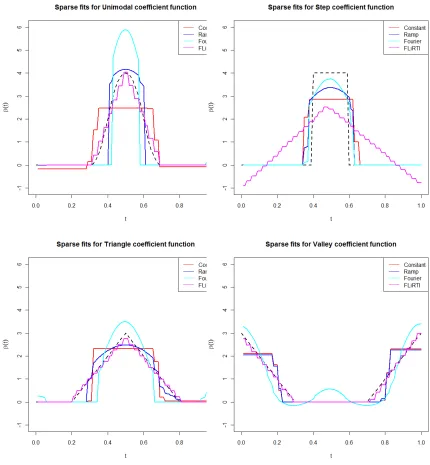
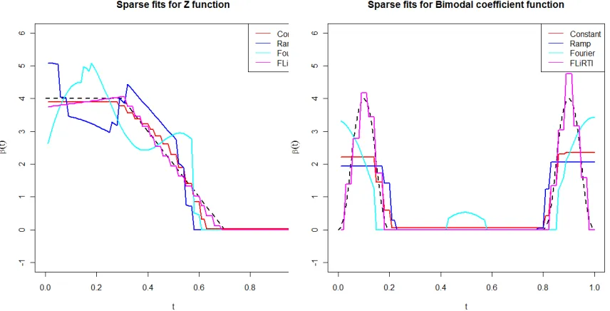
Six coefficient functions defined onT = [0,1]are considered. These can be seen in Figure 2.4. For each coefficient function, we consider sample sizes ofn = 50,100,200,500. Example fits using n = 50 from the 1st order b-spline basis, second stage “ramp”, second stage Fourier, and FLiRTI (d = 2) are given in Figure 2.6 and Figure 2.7. Table 2.1 shows results for all

seven fits (including first stage fits that are not sparse) for the unimodal coefficient function

with n = 50. As we can see from this table, the second stage improves over the first stage forM ISE1 andM ISE2 for both cases. The Type I error rate also improves, while the Type

II error rate gets worse. This same trend was observed across all coefficient functions and all

levels ofn. As such, we do not give results for these first stage estimates in the summaries of results that follow. Additionally, the FLiRTI results withd= 2were generally a bit better than ford= 1, so once again in the interest of space, we only report the FLiRTI results ford= 1.

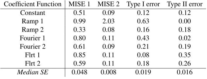
Table 2.1: Simulation results for all methods withβ(t)Unimodal,n= 50,p= 35

Coefficient Function MISE 1 MISE 2 Type I error Type II error

Constant 0.51 0.09 0.12 0.12

Ramp 1 0.99 2.03 0.63 0.00

Ramp 2 0.33 0.08 0.16 0.18

Fourier 1 0.80 0.11 0.43 0.02

Fourier 2 0.61 0.09 0.21 0.19

Flrt 1 0.85 0.11 0.08 0.35

Flrt 2 0.59 0.11 0.18 0.26

(51)

(52)

Figure 2.7: Sparse fits for different coefficient functions

From Table 2.2, we can see that the second stage ramp fit appears to be best overall when the

sample size is smallest. Asnincreases from 50, however, the FLiRTI method improves quickly at identifying the zero-regions, while the two second stage fits from both the ramp and Fourier

basis struggle. Indeed, we see the Type II error rates for both increase while the Type I error

rates stay largely the same. The best overall method may be the single stage fit using the 1st

order b-spline basis with the Fused LASSO. This method consistently has the lowest Type I

error rate, and its Type II error rate is always first or second best. This comes at a price in terms

of MISE 1, but MISE 2 for this method is competitive with the alternatives.

When we look at the fit for the Z coefficient function, (see Table 2.3) we again see the Fused

LASSO methods generally outperforming FLiRTI in terms of MISE 1. This means that these

methods are doing a better job of finding the shape of the Z coefficient function than FLiRTI.

(53)

Table 2.2: Simulation results unimodal coefficient function for different values of n with EBIC tuning. (p= 35)

Error Type Fit n=50 100 200 500

Piecewise Constant 0.51 0.43 0.41 0.32

Ramp 0.33 0.31 0.24 0.22

MISE 1 Fourier 0.61 0.38 0.31 0.17

FLiRTI (d= 2) 0.59 0.41 0.27 0.20

Median SE 0.044 0.037 0.035 0.023 Piecewise Constant 0.09 0.05 0.02 0.01

Ramp 0.08 0.04 0.02 0.009

MISE 2 Fourier 0.09 0.05 0.02 0.01

FLiRTI (d= 2) 0.11 0.05 0.03 0.01

Type I Ramp 0.16 0.19 0.18 0.20

error Fourier 0.21 0.21 0.16 0.14

FLiRTI (d= 2) 0.18 0.11 0.11 0.13

Type II Ramp 0.18 0.20 0.23 0.21

error Fourier 0.19 0.17 0.22 0.20

FLiRTI (d= 2) 0.26 0.22 0.18 0.18

Median SE 0.018 0.017 0.015 0.015

fit with the 1st order b-splines has substantially lower Type II error rates than the others, but it

also has the worst Type I error rates. FLiRTI and the second stage ramp fit appear to find the

best balance of the two types of error for the Z coefficient function.

Also, note that for this table, the results reported are the trimmed means for3%trim on either

side. This is due to the fact that the “ramp” basis produced some large outliers withM ISE2

error rates roughly 4 orders of magnitude larger than the other observations. Due to this

excep-tionally poor first order fit, the second order fit was similarly poor. This is indicative of a larger

(54)

to be somewhat unstable and will occasionally produce large outliers such as those observed

here. While we didn’t find outliers like this with other coefficient functions, the standard errors

for the ramp basis fits tended to be higher than other methods. The take away is that while the

two stage fitting process can improve poor first order fits, if the initial fit is bad enough, the

second stage fit will also be poor. More succinctly, “garbage in, garbage out.”

Table 2.3: Simulation results for Z coefficient function for different values of n with EBIC tuning. (p= 35) Note: Trimmed means reported.

Ramp 0.39 0.11 0.25 0.20

MISE 1 Fourier 1.09 0.66 0.57 0.57

FLiRTI (d= 2) 0.69 0.69 0.88 1.13

Ramp 1.48 0.05 0.02 0.01

MISE 2 Fourier 0.12 0.05 0.02 0.01

FLiRTI (d= 2) 0.11 0.06 0.03 0.01

Type I Ramp 0.24 0.15 0.24 0.19

error Fourier 0.12 0.06 0.06 0.07

FLiRTI (d= 2) 0.19 0.15 0.13 0.13

Type II Ramp 0.10 0.08 0.06 0.07

error Fourier 0.19 0.10 0.22 0.21

FLiRTI (d= 2) 0.08 0.07 0.10 0.12

Median SE 0.06 0.08 0.06 0.08

The Bimodal coefficient function proves difficult for the Fused LASSO-based methods to

model. This is to be expected, since these methods penalize large jumps in coefficient value,

(55)

method. However, MISE 2 is nearly equal across the board, and Type I and Type II error rates

show divergent results, with FLiRTI having very low Type I error but correspondingly high

Type II error, and the Fused LASSO based methods showing the opposite.

Results for the Step, Triangle, and Valley coefficient functions are given in the Appendix.

Table 2.4: Simulation results for bimodal coefficient function for different values of n with EBIC tuning. (p= 35)

MISE 1 Ramp 0.94 0.86 0.84 0.78

Fourier 1.42 1.04 0.92 0.89

FLiRTI (d= 2) 0.86 0.75 0.63 0.61

Ramp 0.14 0.08 0.03 0.01

MISE 2 Fourier 0.12 0.06 0.02 0.01

FLiRTI (d= 2) 0.12 0.06 0.03 0.01

Type I Ramp 0.18 0.21 0.16 0.15

error Fourier 0.28 0.23 0.27 0.23

FLiRTI (d= 2) 0.22 0.19 0.13 0.09

Type II Ramp 0.01 0.01 0.01 0.02

error Fourier 0.06 0.03 0.01 0.00

FLiRTI (d= 2) 0.06 0.09 0.14 0.21

(56)

2.5.3 Sparely Observed Curves with Measurement Error

The previous results assumed the curves were fully observed, which is often unrealistic in

functional data analysis. Here, we perform simulations where each curve is observed sparsely

with small measurement error. On a grid of36fixed time points, we observeUij =Xi(Tij)+δij, where δij ≈ N(0, γ2). Below, we report results from simulations using the Unimodal and Z coefficient function with γ = 0.01,0.025. We estimate each curve using a smoothing spline over the observed time points.

Simulations using the Unimodal coefficient function show that the FLiRTI (d = 2) method is

probably the best of the four estimates looked at. (See Table 2.5.) For this coefficient function,

only the single stage Fused LASSO fit with the 1st order b-spline basis was competitive.

How-ever, note that as the measurement error was increased fromγ = 0.01to0.025, the difference between these two became closer, with the Fused LASSO performing better inM ISE2 and

Type II error and FLiRTI performing better in the other categories.

Table 2.5: Error rates for Unimodal coefficient with measurement error

γ Fit MISE1 MISE2 Type I errror Type II error

Fused Lasso 0.272 0.028 0.291 0.128

0.01 2nd Stage Ramp 0.353 0.035 0.149 0.258

FLiRTI 1 0.458 0.037 0.085 0.331

FLiRTI2 0.268 0.041 0.166 0.158

Fused Lasso 0.361 0.037 0.362 0.123

0.025 2nd Stage Ramp 0.540 0.059 0.207 0.273

FLiRTI 1 0.622 0.065 0.161 0.303

FLiRTI2 0.357 0.068 0.198 0.204

(57)

the Fused LASSO-based methods perform much better than both FLiRTI methods across the

board. Between the two-stage “ramp” basis fit and the single stage 1st order b-spline fit, it is

unclear which is the best. Both have similar M ISE2s, and while the single stage method is

substantially better forM ISE1, its Type I error rate is much worse than the two stage

alter-native. Together with the results from the Unimodal coefficient function simulation, we can

say that the two-stage Fused LASSO method works with some degree of success for data with

measurement error. While its performance relative to FLiRTI clearly depends on the coefficient

function, a single stage fit using 1st order b-splines and the Fused LASSO appears to always

perform pretty well.

Table 2.6: Error rates for Z coefficient function with measurement error

γ Fit MISE1 MISE2 Type I errror Type II error

Fused Lasso 0.182 0.074 0.477 0.011

0.01 2nd Stage Ramp 0.492 0.079 0.099 0.032

FLiRTI 1 1.363 0.106 0.854 0.074

FLiRTI2 0.909 0.108 0.559 0.045

Fused Lasso 0.209 0.090 0.422 0.014

0.025 2nd Stage Ramp 0.518 0.096 0.145 0.035

FLiRTI 1 1.419 0.130 0.791 0.072

FLiRTI2 0.929 0.126 0.555 0.045

For this simulation, the measurement error included was very small. (The standard deviation

ofγ was0.01,0.025 compared to a standard deviation of4for the basis function coefficients used to generate the curves.) Since the error was small, the results were still reasonable, but we

New Techniques for Functional Data Analysis: Model Selection, Classification, and Nonparametric Regression.

ABSTRACT

BIOGRAPHY

ACKNOWLEDGEMENTS

TABLE OF CONTENTS

LIST OF TABLES

LIST OF FIGURES

Chapter 1

Introduction

1.1

Regression

1.1.1

Penalization Methods

1.1.2

Nonparametric Regression

1.2

Functional Data

1.2.1

Regression for functional data

1.2.2

Notation for functional data

1.2.3

Functional Principal Components

1.2.4

FPC for Sparse and Irregularly Sampled Data

1.2.5

Fitting Functional Regression Models

1.3

Dissertation Outline

Chapter 2

Model Selection for Functional Data

2.1

Motivation

2.2

Functional Regression

2.2.1

General Approach

2.2.2

Existing Methods

2.3

New Methods

2.3.1

Two-stage fitting

2.3.2

Sparsely Observed Trajectories and Measurement error

2.3.3

Summary of Algorithm

2.4

Computational issues

2.4.1

Tuning for

λ

and

λ

2.4.2

Numerical integration and other issues

2.5

Simulations

2.5.1

Assessing the quality of a fit

2.5.2

Simulation Results

2.5.3

Sparely Observed Curves with Measurement Error