On Shape Description and Optimization for Object Classification

(1)

POLIANNIKOV, OLEG VICTOROVITCH. On Shape Description and Optimization for Ob-ject Classification. (Under the direction of Prof. Hamid Krim)

(2)

by

OLEG V. POLIANNIKOV

A dissertation submitted to the Graduate Faculty of North Carolina State University in partial fulfillment of the requirements for

the Degree of Doctor Of Philosophy

ELECTRICAL ENGINEERING

Raleigh February 2003

APPROVED BY THE ADVISORY COMMITTEE:

Chair: Prof. Hamid Krim

Member: Prof. Jean-Pierre Fouque

Member: Prof. Brian L. Hughes

(3)

(4)

PERSONAL BIOGRAPHY

(5)

ACKNOWLEDGMENTS

Working on this thesis has been many things, but first and foremost it has been four years of my life. Here I would like to acknowledge people who helped me not only survive through that time, but turn it into an exciting and unforgettable experience.

A lot of credit is certainly due to my advisor Prof. Hamid Krim. I would like to thank him for suggesting the problems to work on, offering me his ideas, making an often humanly impossible effort to keep me focused on the goals and finally paying my bills. I would further like to express my gratitude to the members of my committee: Prof. Brian L. Hughes, Prof. J. Keith Townsend and Prof. Jean-Pierre Fouque for their willingness to serve on the committee as well as constructive and friendly suggestions. I thank Prof. Arne Nilsson for having served on my committee during the initial phase of my program and Prof. H. Joel Trussell for having being a member of the committee as well as for the enormous amount of time that he had spent with me while I was working on the first part of this thesis.

I would like to thank the current as well as former students from our group whom I have enjoyed spending time with all these years. Those include Dr. Yun He, Dr. Bilge Karacali, Dr. Gozde Bozkurt Unal, Dr. Yufang Bao, Dr. A. Ben Hamza, Viraj Mehta, Aysegul Gunduz, Yang Wu, Sajjad Baloch, Christina Hammoc and many others. I’m grateful to all these people for providing me a great work environment as well simply being my good friends all this time.

(6)

LIST OF FIGURES

Figure Page

2.1 Synthetic silhouette of a B-2 plane. . . 17 2.2 Samples with the same values but different locations correspond to different signals. . 24 2.3 Orientation of a pair{τ(t), γs(t)}remains the same for allt∈[a, b]. . . 28

2.4 A curve and its admissible set. . . 29 2.5 Given a polar center a curve can be reconstructed from any samples as long as their

number is sufficient. . . 31 2.6 A curve is sampled and then perfectly reconstructed from the sampleswithout using

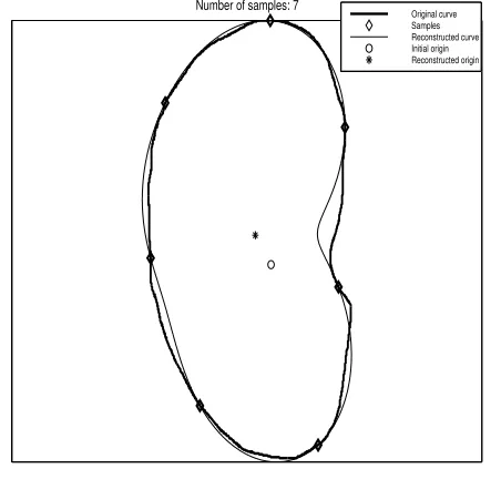
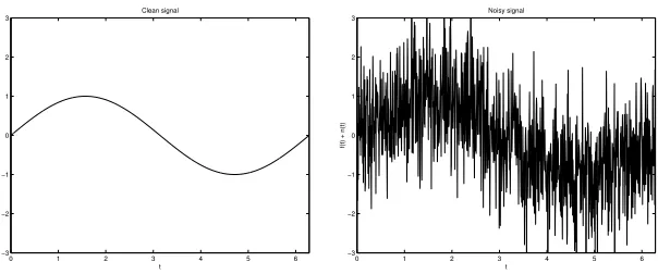
any additional information. . . 34 2.7 A good approximation of a map of Germany may be obtained from as few as 15 samples. 38 2.8 A contour of a human kidney can be recovered from only 7 samples. . . 39 2.9 A contour of a human brain can be recovered from only 19 samples. . . 39 3.1 Example of a clean signal and the same signal corrupted by additive Gaussian noise. . 44 3.2 Many functionals exhibit multi-modal behavior, which means they have several local

extrema. . . 45 3.3 When the local minimum is found via a deterministic descent it is possible to identify

the exact location of the extremum much simpler than in the case of a stochastic diffusion. . . 56 3.4 A new implementation of simulated annealing for a signal filtering functional yields

(9)

Figure Page 3.6 A new implementation of simulated annealing for an image filtering functional yields

faster convergence to the global minimum. . . 59

3.7 Higher energy level yields more visible noise while lower energy level yields cleaner image. . . 59

3.8 Evolving a perturbed version of the original signal may yield better minimization results. . . 61

4.1 Examples of discrete objects. . . 66

4.2 Pinhole camera. . . 67

4.3 Arbitrary coordinate frame. . . 71

4.4 Rotation parameters. . . 71

4.5 Frontal and skewed views of the same shape. . . 73

4.6 Projective transformations preserve collinearity of points. . . 74

4.7 Construction of skeleton. . . 77

4.8 Example of skeleton of view. . . 78

4.9 Skeleton signature. . . 80

4.10 Reconstruction of a view from a skeleton. . . 83

4.11 Different choice ofx1 affects only the width of the underlying shape. . . 84

4.12 Noise-free and noisy skeletons. . . 87

4.13 Realizations of noisy skeletons. . . 89

4.14 Groups of correlated points in a skeleton. . . 91

4.15 Skeleton points correlation coefficients are functions of only4 shape points, not the entire shape. . . 93

(10)

Appendix

Figure Page

(11)

Chapter 1 Preface

1.1 Problems Motivation, Formulation and Main Results

Shape analysis is a common term which refers to a whole class of theories, methods and tools whose fundamental goal is to extract useful geometric information about an object from available data. A problem of such generality is by definition so broad and ambitious in nature and so vital to many applications, that it has attracted a lot of attention of people from different areas, such as differential geometry, computer vision, functional analysis, optimization, stochastic processes just to name a few.

(12)

of the steps mentioned above constitutes in its own right a large and complex problem, which needs to be addressed, its exact formulation or the applicability of any particular tool or method are often carried out within the global context.

In the general description of the problems we have investigated in this thesis, we briefly review some of the related works, which have appeared in the literature. Each one of these problems constitutes a milestone within the big picture goal.

1.1.1 Discretization of Continuous Objects

Shapes of observed objects naturally arise in images and in other context. Any3−Dobject, such as an airplane, tank, human kidney or brain is an example of shape. Mathematically we can think of the boundary of an object as being its shape. A lot of objects, such as airplanes or tools such as wrenches, are almost two-dimensional as their width to length ratio is rather small, which heads one to think it is reasonable to assume them as two dimensional shapes. Imaging a3₋D object naturally gives rise to another2−Dobject (its image), with its boundary becoming another example of a2₋Dshape.

(13)

pre-processing ensures no loss of geometric information and hence the higher quality of resulting methods. It is clear that these advantages may also be sources of major challenges, as a shape space of any significance, i.e. a family of shapes of interest, is very large and of infinite dimension. This further simplifies complicates the theoretical analysis and yields severe computational problems in the course of implementation.

Confronting these challenges has had mixed results, and promising new avenues have recently emerged. Specifically, a novel idea that has been gaining acceptance is that our interest in shape should often be limited to a set of a relatively small number of key features. For example, the estimation of the position of an airplane in the air or even to classify it up to a rather narrow class may only require the position of its head, tail and ends of the wings. Information about the entire surface would turn out to be redundant and any computations required to obtain it could be considered wasted resources. Reducing a shape to a handful of its key point, commonly referred to as landmarks, with no/minimal loss of information is hence not only promising but holds a great potential to significantly simplify any problem related to shape understanding. Furthermore, as it has been shown by Kendall, Mardia and others ([23, 24, 11, 17]), such a framework enables us to build a elegant and powerful theory of discrete shapes capable of encompassing both the deterministic as well as statistical settings.

(14)

persists even if a priori information about the representability of a continuous shape in terms of a finite number of discrete points is present. In the first part of the thesis we address the problem of sampling of a continuous planar closed contour. This problem has been addressed in the litera-ture, and perhaps the most common approach has been based on splines ([36, 29]). While splines achieve relatively good performance in discretizing a curve, they do not provide a one-to-one cor-respondence between a a continuous curve and its discrete counterpart.

In this work, we show that a choice of a coordinate system or a parameterization for the curve plays a crucial role in the construction of a sampling algorithm. Unlike the case of a standard1−D or2₋Dsignals, curves and surfaces do not yielduniquefunctional representations. The latter case entirely depends on a choice of a parameterization for the given geometric object. By providing a consistent way of associating to each curve or surface a unique functional representation, which in turn requires a pre-determined coordinate system, we avoid any ambiguity. Sampling of the resulting function would then have to account for the function itself as well as for the coordinate system, with respect to which it was obtained.

(15)

fixing a coordinate system essentially turns a planar curve into a1−Dfunction. This in turn leads to be optimistic about a possible generalization of the existing theory of sampling1₋Dfunctions to the case of curves.

The major obstacle to such generalization is the fact that while in the standard1−Dtheory, samples of a function only carry the information about the function itself, they should, for the case of curves, provide knowledge about the particular coordinate system that the curve was represented in. For the polar coordinates, such knowledge includes the location of the polar center. Its position has to be recoverable from the samples of the curve, so that the coordinate system could be recon-structed first without any additional information, and then be used together with1₋D sampling theory to recover the functional form of the curve. Our sampling algorithm meets those require-ments and is applicable to any curve representable in polar coordinates and satisfying additional smoothness constraints described in details in the chapter.

(16)

This optimization problem is applicable to and can be solved ([16]) for a much broader class of curves, yielding sufficiently accurate approximations.

Finally, by using the spherical coordinates instead of polar ones, the results of this chapter are easily generalized to the case of3−Dclosed surfaces.

1.1.2 Signal and Image Filtering Using Stochastic Optimization

Many tasks in image processing in general and shape analysis in particular can be formulated as optimization problems. To an image, for instance, we can associate its cost that somehow measures the amount of noise in it. The stronger is the noise, the larger that cost would be. Filtering can then be defined as modifying the original image so as to reduce its cost. Image segmentation can also be expressed as a cost minimization problem, where now for a given image, possibly consisting of several pieces, to any curve we associate the cost which is inversely proportional to a similarity between image regions bounded by that curve, however that similarity may be defined. Assuming that homogeneous regions correspond to different objects on the image, it is clear that the closer the curve would resemble their boundaries, the smaller the cost would be.

Mathematically, a cost is defined as a functional H (f), where _f _∈ F is a signal, image,

curve etc, spanning some admissible space F. The problem is then to find the optimal signal

corresponding to the minimal cost, i.e. findf0 = arg min

f∈F

H (f).

Digital signals, images and even more geometrically complex structures, such as curves and surfaces, are conveniently modelled as vectors from some possibly high but finite dimensional Euclidean space Rd. A cost functional is then represented as a map H _: Rd _→ R from that

(17)

necessary condition for its minimizer is ∇H _(f₀) = 0, where the symbol _∇ denotes the usual

gradient. A standard approach for finding a point satisfying that condition is by using the gradient descent method, where we continuously descend in the direction of the gradient until the bottom is reached.

There are numerous problems with the gradient descent method, and the most challenging be-ing that of a functional havbe-ing more than one local minimum, i.e. several points satisfybe-ing the necessary condition, in which case the method is only capable of finding the nearest local min-imum but not the global optimizer. A class of methods where the deterministic gradient-based search for an optimum is replaced by a stochastic procedure falls under the class of stochastic opti-mization techniques. An intuitive but rather simplistic and sometimes misleading way of thinking of stochastic optimization is in the absence of any guidance, one makes a random but hopefully educated guess, which in the long run averages to the proper direction.

(18)

energy of that change, as a function of time is sometimes referred to as the temperature schedule, a term which came from physics where the technique was first described and applied.

It has been shown that if the temperature monotonously and very slowly decays to zero, the system converges in probability to its optimal state. Despite its theoretical optimality, the practical and straightforward implementation of this technique has proven inefficient due to prohibitively slow convergence. The initially proposed temperature schedule was such that for any reasonable time period, the temperature level remains significant causing the system to keep changing its state without converging. It is important to note that a slow decay of the temperature is crucial for the convergence to take place, therefore implying that no faster decaying schedule is theoretically possible. In light of this phenomenon, research that followed up was primarily concentrated on modifying the algorithm while preserving the central idea of using stochastic perturbations to allow the system to escape local minima.

We propose to investigate the problem of coming up with a simulated annealing-based opti-mization technique, which would be

• suitable for a broad class of functionals;

• easy to implement;

• fast.

(19)

forcing more aggressive search by increasing the temperature if the system fails to improve on the current state for a long period of time.

The key idea of the proposed algorithm is the notion ofscale of search. Intuitively, if a func-tional is such that its local minima or at least principal modes are sufficiently far apart, the search should be conducted at a coarser scale, while if local minima are closely clustered together, the functional has to be explored at a much finer scale so as to minimize the chance of missing the mode containing the global minimum. While for any given functional it may be possible to find a corresponding optimal scale of search, for an arbitrary cost function the temperature sched-ule should automatically adapt to its behavior. We propose to start the search by exploring the functional at a finer scale first, which corresponds to a lower temperature, and then progressively increase the latter thus coarsening the evolution until a lower cost state is found.

The conducted experiments confirm that this intuitive argument is justified and performs well in practice. Furthermore, the absence of a complicated acceptance - rejection algorithm used by some other simulated annealing-based techniques is the key to the ease of implementations, which in turn enables us to apply the same algorithm to different functionals and achieve a satisfactory performance.

1.1.3 Identification of an Object from a Single Image

(20)

features of known objects. Provided that database is sufficiently complete, that would allow us to recognize the object.

We have argued earlier that a shape analysis is greatly simplified when shapes are represented as discrete entities in terms of their landmarks. In this part of the thesis, we will assume that an object is represented as a collection of discrete points{Xi} in 3−D space, and its image is a

2₋Ddiscrete shape_{xi}. Obviously, an image{xi}is a function of the object and the camera.

A recognition mechanism is then defined as any function of the image, f _{xi}

, which remains invariant to the choice of camera. In addition, a good recognition mechanism should possess the following properties.

• The image of the functionf(_·)should have the smallest dimension possible.

• While it is typically not necessary for a function f(_·) to be bijective, it is desirable that it would contain as much information about its argument as possible, so as to better discrimi-nate between different objects.

• The recognition mechanism should be robust to noise in the data. Most recognition

(21)

Projective geometry provides a very elegant and convenient framework for the problem of recognition of a discrete shape ([15]). Let the set of pointsXi ∈ P3 denote an object lying in the

3₋Dprojective space, andxi ∈P2 be its corresponding image. The standard “pin-hole camera”

model then assumes that the image and the object are related through the equationxi =PXi, where

Pis a₃×₄matrix of a linear projective transformation. It can then be deduced that different images of the same object,xiandx0i, corresponding to camerasPandP0respectively, are related through a

linear transformation fromP2to itself (projective transformation), defined by some matrixH. The above suggests that to construct a recognition scheme, we should search for invariants of projective transformations ([9, 33, 37, 38, 39]). A variety of invariants have been proposed in an extensive research in the area. It has been proven that assumptions about the class of objects of interest are required for any recognition to proceed ([6]). The idea is to therefore impose constraints that would be sufficiently restrictive to make the recognition feasible, and sufficiently broad to encompass the class of shapes of interest in our applications.

(22)

The same holds true for the skeletons of those views, i.e. the skeleton of the view{xi}is the

pro-jective image of the skeleton of another view{x0_i_}through some1₋Dprojective transformation. Furthermore, we formally show it that skeletons contain virtually as much geometric information about the original object, as the views. The problem of object recognition can therefore be reduced to classification of possible view skeletons.

Recall that a skeleton consists of several collinear points. The famous projective invariant of collinear points is the so-called cross-ratio. A cross-ratio is a function of four collinear points defined in terms of ratios of distances between them, which remains invariant to any projective transformation on those points. If a skeleton contains more than4different points, we can construct a vector of cross-ratios by taking different 4-tuples of points. That vector would obviously be projectively invariant. To summarize, given a view we can construct its skeleton which in turn gives rise to a vector of cross-ratios. The latters only depend on the initial object, and not on any particular image. Furthermore, this invariant captures almost all geometric information about the object, which makes it a good candidate for a recognition technique.

(23)

While completely computing the multi-dimensional distribution of the signature vector is still an open problem ([34]), we show that under the assumption that the noise in data is independent and gaussian with zero-mean and identical variance, optimal identification is still possible, i.e. while it is certainly not feasible to do a perfect recognition in the noisy environment, for a given view, we can derive an optimal estimate of its skeleton, which would in turn allow us to compute the estimates of the cross-ratios. This statement is based on a proposition, which states that an independent gaussian noise in the data points leads to skeleton points becoming gaussian with the mean coinciding with the true skeleton and some covariance matrix Σ. The estimate of the true skeleton is then found by applying the generalized linear fit to the noisy skeleton points.

1.2 Thesis Organization

(24)

Chapter 2 Sampling Closed Planar Curves and Surfaces

2.1 Introduction

Sampling theory has a long history of development ([4, 55, 62]). The classical sampling theo-rem, which provides the basis for reconstructing bandlimited1−Dsignals from discrete samples, was first proved by Cauchy, rediscovered by Whittaker ([48]) and Kotelnikov ([28]), and finally applied to problems of communications by Shannon ([49]), which ultimately resulted in the ”digi-tal revolution”. The theorem is remarkable in that it allows converting an analog signal satisfying certain class constraints into a discrete sequence of numbers without any loss of information. Its mathematical statement is as follows.

Theorem 2.1 If a function f : R _→ R is bandlimited to _ω_max _< π

T, then it can be exactly

reconstructed from its values at sampling pointstn =nT:

f(x) =

+∞

X

n=−∞

f(nT)sincx T −n

, x_∈R_. (2.1)

(25)

represent signals relative to them. Furthermore, it was shown that one might take advantage of stable representations of a signal with its coefficients with respect to systems with redundancy as opposed to orthogonal bases. That theory gave rise to the notion of frame and delivered many powerful sampling techniques ([2, 1]).

In this chapter we consider the problem of sampling a closed planar curve or a 3−Dsurface. Just like in the case of1₋Dsignals, the ability to convert a continuous contour to a collection of discrete points is extremely desirable and yields a number of useful applications. If the informative content of an image is limited to a single shape, then sampling the boundary of the object as opposed to the entire image may result in significant increase of compression efficiency.

On the other hand, when a shape is analyzed in the context of computer vision, then the im-portance of being able to find a discrete representation cannot be overemphasized. While there exists a number of methods dealing with continuous curves, the latter must often come from a very narrow class, e.g., quadrics ([56]). At the same time representing shapes as arrays of points is fundamentally simpler, and therefore a richer theory exists for such scenarios ([11, 50, 23]).

The main obstacle we have to tackle when sampling a curve is lack of itsa priorigiven func-tional form ([41]). As will be discussed in detail later, what we normally observe is an image of a curve as opposed to the curve itself. That creates a problem of finding a parametrization that could be run through a sampling algorithm. Since a type of parametrization needs to be defineda priori

(26)

This chapter is organized as follows. Our focus is mainly concentrated on2−Dcurves. Section 2.2 provides a general background about planar curves. Its purpose is to fix the notation as well as provide the insight as to the fundamental differences between1₋Dsignals and planar curves from the point of view of sampling theory. In Section 2.3 we formulate the problem we address in this chapter, and describe in detail the solution that we propose, which includes class-constraints on curves, sampling and reconstruction algorithms and present examples of applying those algorithms to idea curves. Technical proofs are moved to Appendix A for the sake of clarity.

In practice, most if not all curves do not exactly satisfy anya priorigiven conditions. It follows then that no technique can provide a perfect sampling and reconstruction of realistic curves. In light of this, in Section 2.4 we propose an optimization technique which yields an optimal approximation to an original curve. We show that it is consistent with the sampling theorem for class-constrained curves in the sense that the latter becomes a particular case of the former.

Results obtained for2−Dcurves can easily be generalized for3−Dsurfaces. A brief summary of results for3₋Dis presented in Section 2.5. Section 2.6 concludes the chapter by providing the final remarks.

2.2 Planar Curves

(27)

Figure 2.1 Synthetic silhouette of a B-2 plane.

−40 −30 −20 −10 0 10 20 30 40 −10

0 10 20 30 40 50 60 70

about the nature of the curve. Note that if we are given a graph of a 1₋D signal, then a very specific coordinate system, namely Cartesian, is attached to it even if not explicitly mentioned. We will give the following definitions ([3, 19]).

Definition 2.2 A path (parameterized curve) is a continuous functionγ : [a, b]⊂R_→R2, i.e.,

γ(t) = x(t), y(t)∈R2_{, t}_∈_{[a, b], γ} _∈_C _{[a, b]}_. (2.2)

Heret, which varies in[a, b], is the parameter of a curve.

Definition 2.3 The subsetC _⊂R2defined by

C ₌_Im(γ)_≡_γ _{[a, b]} _≡_γ(t)_|_t_∈_{[a, b]} (2.3)

is called the image of a pathγ(·).

The setC is what we really call a curve in everyday life. It is therefore intuitive that the setC

(28)

The following construction assures thatC is in fact independent from a parameterization so long

as the latter belongs to an admissible class of paths.

Definition 2.4 Two pathsγ1(t) : [a, b] → R2 andγ2(τ) : [α, β] → R2 are said to be equivalent

(writeγ1 ∼γ2), if there exists a change of variablet=t(τ), satisfying the conditions

1. t: [α, β]→[a, b]is a bijection between the two intervals;

2. tandt−1 _{are continuously differentiable, i.e.,}

t_∈C1 [α, β], t−1 _∈ C1 [a, b]; 3. The two parameterizations have the same direction, i.e.,

d

dτt(τ)>0, ∀τ ∈[α, β], such that

γ1 t(τ)

=γ2(τ), ∀τ ∈[α, β]. (2.4)

It easily follows from Definition 2.4 that equivalent paths have the same image.

Theorem 2.5

γ1 ∼γ2

⇒ Im(γ1) =Im(γ2)

. (2.5)

(29)

Definition 2.6 Letγ0 : [a, b]→R2 be a path. Then the equivalence class

C ={γ _|γ _∼γ0} (2.6)

is called a curve with the representativeγ0.

Theorem 2.5 asserts that the image of a curve is uniquely defined.

Definition 2.7 LetCbe a curve, andγ0 ∈C. Then by definition

Im(C)_≡Im(γ0). (2.7)

Definition 2.8 A curveC is called closed if it contains at least one parametrizationγ0 : [a, b] →

R2, which is closed, i.e.,_γ₀_{(a) =}_γ₀(b).

One easily establishes thatallelements of a closed curve are closed parameterizations.

Definition 2.9 A closed curve C is called Jordan if it does not intersect itself except at the end points, i.e., ifγ0 : [a, b]→R2 is its parametrization, andt1 < t2 then

γ0(t1) =γ0(t2)

⇒t1 =a, t2 =b

. (2.8)

In the remainder of the chapter, we will focus exclusively on Jordan curves.

(30)

Definition 2.10 Letγ : [a, b]→R2_{, γ} _∈_C1 _{[a, b]}_{, γ(t) =} _{x(t), y(t)}_{, t}_∈ _{[a, b]}be a path and

t0 ∈[a, b]. Then the unit tangent vector to the path at the pointγ(t0)is a vectorτ(t0)defined as

τ(t0) =

γ0_(t

0)

kγ0_(t

0)k ∈

R2_, (2.9)

where

γ0(t0) = x0(t0), y0(t0)

, _kγ0(t0)k=

q x0_(t

0)2 +y0(t0)2. (2.10)

As was noted earlier, it can be easily shown that the notion of a unit tangent vector to a curve is geometric, i.e., it does not depend on a particular parameterization of the curve. More precisely, the following theorem holds.

Theorem 2.11 Let γ1(t) : [a, b] → R2 and γ2(τ) : [α, β] → R2 be two equivalent paths, i.e.

γ1 ∼γ2, such thatt=t(τ)is a change of variable satisfying all the conditions listed in Definition

2.4. Letτ1(t),τ2(τ)be tangent vectors to pathsγ1andγ2at pointsγ1 t(τ)

andγ2(τ)respectively.

(Note thatγ1 t(τ)

=γ2(τ).) Then

τ1 t(τ)

=τ2(τ). (2.11)

The proof of this theorem can be found in [19]. We will make use of this theorem in later sections of the chapter.

2.3 Sampling Planar Curves

2.3.1 General Finite Sampling Problem

(31)

description and solution of the problem will not only be rigorous and unambiguous, but it will also help us contrast and compare the relevance of traditional sampling theory of 1₋D and 2₋D signals to the problem we have at hand.

To proceed with the formulation of the finite sampling problem for an arbitrary signal, we state the following definition.

Definition 2.12 Let f : X _→ Y be a signal (function). Completely specifying the sampling problem of this signal entails imposing conditions on f, such that it is possible to find a triple

(N,X_,I), where_N _∈Nis a number of samples,X _{≡ {}_x₁_{, . . . , x}_N_{} ∈}_XN _{is a collection of}_N

distinct samples, andI is an interpolation function (method of reconstruction): I _:_XN _×_YN _×

X _→Y, such that

I _x₁_{, f(x}₁_{), . . . , x}_N_{, f(x}_N_);_x₌_f(x), _∀_x_∈_X. (2.12)

The reader may find the above definition too abstract. However, it is extremely important to for-mally specify the problem we are going to be addressing. This definition also reveals the minimal information needed in order to formulate a sampling theorem. The following well-known theorem is a classical example of a solution to a1₋Dfinite sampling problem.

Theorem 2.13 Letf :R_→Rbe a₁₋_Dsignal. Suppose also that it is periodic with a

fundamen-tal period2π and bandlimited, i.e., there existsN _∈ N(for the sake of simplicity we will assume

N even) andc₋N

2, . . . , c

N

2 ∈C, such that

f(t) =

N/2

X

n=−N/2

(32)

Then if t1, . . . , tN+1 ∈ R is a collection of N + 1 arbitrary but distinct points on the real line

and f(t1), . . . , f(tN+1) the corresponding sample values of f(t), we can reconstruct the signal

f(t), and the interpolation function, I, is defined by the right side of Equation2.13, where the

coefficients{cn}n=−N

2,...,

N

2 are the unique solution of the following system of equations.

       

f(t1)

...

f(tN+1)

        =        

ei(−N2)t1 · · · ei

N

2t1

... ... ...

ei(−N2)tN+1 · · · ei

N

2tN+1

        ·        

c₋N

2 ... cN 2         . (2.14)

The reader may refer to [32] among others for the proof of this theorem. It easily follows from the fact that anyN+ 1samples yield a linear system of equations with respect toN+ 1signal Fourier coefficients, which is full-rank and thus has a unique solution. The Fourier coefficients, in turn, completely define a signalf(t)(see, for example, [45]).

Definition 2.14 Letf :X _→Y be a given signal. We will say that a point

y_∈Im(f) (2.15)

is an incomplete sample off onX.

Definition 2.15 Letf :X _→Y be a given signal. We will call a pair

x, f(x)_∈X_×Y, (2.16)

a complete sample off onX.

(33)

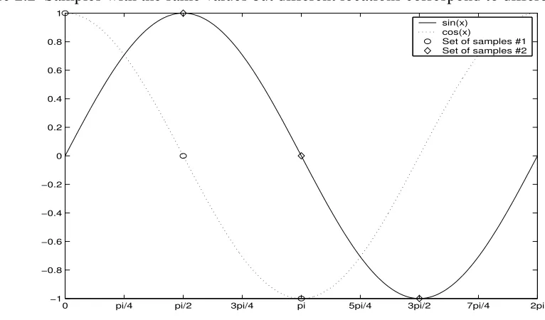
its complete samples. The following simple example demonstrates that the sample locations are critical.

Consider again a1₋Dbandlimited signalf(t), satisfying all of the conditions from Theorem

2.13withN = 3. Then if we are given any 3 complete samples, Theorem2.13guarantees that we will be able to uniquely reconstructf(t). On the other hand, if we were given incomplete samples, then by varying the locations of those samples we would be able to construct an infinite number of signals, satisfying all the required conditions, e.g., if

f(t1) = 1, f(t2) = 0, f(t3) =−1,

then the locations

t1 = 0, t2 =

π

2, t3 =π yieldf(t) = cost, but for

t1 =

π

2, t2 =π, t3 = 3π

2 ,

the formula for the signal would becomef(t) = sint(See Figure 2.2).

This very simple example underlines the difficulty we encounter when formulating a sampling problem for planar curves as we discuss next.

2.3.2 Sampling Closed Curves: Formulation

Recall, that a closed planar curve C is a class of equivalent (closed) parameterizations of the same imageC. We formulate the sampling problem for the curve_Cas follows. Find a

(34)

Figure 2.2 Samples with the same values but different locations correspond to different signals.

0 pi/4 pi/2 3pi/4 pi 5pi/4 3pi/2 7pi/4 2pi −1

−0.8 −0.6 −0.4 −0.2 0 0.2 0.4 0.6 0.8 1

(35)

which satisfies some conditions so that a finite number of complete samples results yielding a reconstruction ofγ(_·).

To proceed, it is important to make the following observation. A complete sample for a curve has the form t;γ(t) ≡ t;x(t), y(t). In practice, however, all we have is a set of point

(xi, yi) N

i=1, which do not constitutecompletesamples. In fact, a closer consideration reveals that

these samples are not evenincompleteas for arbitrary points on the plane(xi, yi) N

i=1there is no

information about the parametrization at hand or its domain. The following two steps are in order to mitigate such a limitation.

• Make additional assumptions about the nature of a curve, namely about thetypeof coordinate system, this curve is represented in.

• Make the information of the coordinate system selection part of the sample specification so

as to avoid any potential ambiguity presenting a closed curve and subsequentles.

2.3.3 Curves Representable in Polar Coordinates

As was

(36)

To address the representation issues of closed (Jordan) curves, one natural reference system which surfaces is that of polar coordinates. Assuming that such a curve representation exists, its seemingly restrictive scope quickly pales next to its merit in suitability as well as adaptability to a wide array of settings. In the case of interest herein, we adopt a polar parametrization of a given curveCand next discuss the technical conditions which underly its existence.

Definition 2.16 Suppose we have a curve C. If for a given point γ0 ≡ (x0, y0) there exists a

functionr(θ) : [0,2π]_→R2, such that the curve_Ccan be parameterized according to

γ(θ) =γ0+ r(θ) cos(θ), r(θ) sin(θ)

, θ_∈[0,2π], γ(0) =γ(2π), (2.17)

then we callγ0 an admissible (polar) center ofC.

While such a definition does not uniquely specify an admissible center of a curve, it allows us to ad-dress the existence issue, which in turn affords our constructing of curves whose class membership is easily carried out.

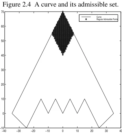
Given a curveC, and using the above definition, we may proceed to determine the admissibility of any point(x0, y0) by ensuring that every half-line originating at this point intersects C at one

and only one point. To alleviate the computational load such a procedure may entail, we state the following theorem which forms the basis for a more efficient search of admissible points.

Theorem 2.17 LetCbe a smooth curve,(x0, y0)∈R2, and`- half-line starting from(x0, y0)and

intersecting the image ofC, setC, in at least two points. Then there exists another half-line_`tthat

(37)

The proof of this theorem can be found in the Appendix A.

It is important to note that the existence of a tangent half-line to a curve originating at a point

(x0, y0)does not guarantee the non-admissibility of the latter as a center for the curve. It does,

however, as further discussed below, rule all of those points out of the set from further consideration and hereby identify a so-called regular admissible set.

Definition 2.18 LetCbe a curve and (x0, y0) ∈R2 be a point. Then this point is called a regular

admissible center if there exists no half-line`going from(x0, y0)and tangent toC. A collection

of all regular admissible centers will be called the admissible set of the curveCand denotedA_C.

To simultaneously qualify the membership of any selected point (x0, y0) to AC and avoid a

computational explosion, the following describes an easily implementable procedure.

Theorem 2.19 Let C be a curve, and γ : [a, b] → C be its parametrization. For any _t _∈ _{[a, b]}

defineτ(t)- a unit tangent vector to γ at a pointγ(t), andγs(t)- a vector connecting the points

γ0 ≡(x0, y0)andγ(t)≡ x(t), y(t)

, i.e.,

γs(t) = x(t)−x0, y(t)−y0

, t _∈[a, b], (2.18)

whereγ(t)_≡ x(t), y(t)(see Figure 2.3). Thenγ0 ∈AC if and only if the orientation of the pair

of vectorsτ(t), γs(t) is constant (non-zero) for allt∈[a, b]. The latter condition means

sgn    

γ1(t) γ2(t)

τ1(t) τ2(t)

  

=const6= 0, ∀t ∈[a, b], (2.19)

whereγ(t)≡ γ1(t), γ2(t)

T

, τ(t)≡ τ1(t), τ2(t)

T

(38)

Figure 2.3 Orientation of a pair{τ(t), γs(t)}remains the same for allt∈[a, b].

r_0 r(t_1)

r(t_2) τ τ

γ

(t_2) (t_2)

(t_1)

See Appendix A for the proof of this theorem. Appendix B contains more details regarding the numerical implementation of the test for admissibility based on Theorem 2.19.

In practice, a continuous curve is, of course, a polygon with a large number of vertices and ever smaller edges, and significantly simplifies the exhaustive search as called by Equation (2.19). In addition, as we show next, the structure ofA_C may be used to advantage in avoiding to have to

check the totality of points individually.

Theorem 2.20 LetC be a curve andA_C be its admissible set. ThenA_C is convex, i.e.,

γ1, γ2 ∈AC

⇒[γ1, γ2]⊂AC

, (2.20)

where

[γ1, γ2] =

αγ1+ (1−α)γ2 |α∈[0,1] . (2.21)

The proof is presented in the Appendix A. A fast and simple approximation of A_C may, for

(39)

Figure 2.4 A curve and its admissible set.

−40 −30 −20 −10 0 10 20 30 40 −10

0 10 20 30 40 50 60 70

(40)

2.3.4 Sampling and Reconstructing Curves: Algorithms

Provided that a non-empty admissible set A_C exists, as spelled out above, our goal in this

section is to describe practical algorithms enabling us to sample closed curve and reconstructing them. Specifically, when given a curveC, we have to, subject to any other additional constraints, identify and acquire its appropriate samples, which will also allow us to reconstruct it.

SupposeC is a curve andγ0 ∈ AC. Then by definition there exists a polar parameterization

r(θ), θ ∈[0,2π] of the curveC. Since,r(θ)is a1−Dsignal, we may therefore apply Theorem 2.13 to obtain the following result.

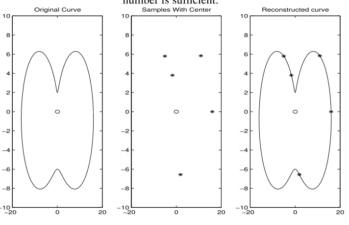
Theorem 2.21 Suppose that we have a curveCandγ0 ∈ AC. Letr(θ)be a polar representation

ofC centered atγ0. Then ifr(θ)is bandlimited, and there existsN ∈N, such that

r(θ) =

N/2

X

n=−N/2

cneiθn, (2.22)

thenr(θ)can be reconstructed from anyN + 1samples (See Figure 2.5).

The reconstruction formula follows from Theorem 2.13. A few remarks regarding the last result are in order.

• Note that this result is not a finite sampling theorem as it heavily relies on a given pointγ0.

Assuming such knowledge is quite unnatural, since in practice we are given only samples of a curve, and thus it is impossible to use this theorem.

• Providing the polar center of a curve explicitly is often undesirable because of noise that

(41)

Figure 2.5 Given a polar center a curve can be reconstructed from any samples as long as their number is sufficient.

−20 0 20 −10

−8 −6 −4 −2 0 2 4 6 8

10 Original Curve

−20 0 20 −10

−8 −6 −4 −2 0 2 4 6 8

10 Samples With Center

−20 0 20 −10

−8 −6 −4 −2 0 2 4 6 8

(42)

transmitted over a digital channel. It then would not greatly reduce the efficiency of trans-mission if we simply addedγ0 to transmitted samples. The downside of this approach is in

thatγ0becomes the bottle-neck of the system, since any error added to it, would significantly

affect the reconstructed curve.

Our goal is now to come up with a sampling technique that would allow us to extract the polar coordinate system from samples in a reliable manner. Recall, that Theorem 2.13 states that a bandlimited signal can be reconstructed from any (possibly non-uniform) samples so long as their number matches the bandwidth of the signal. We show that it is possible to use this freedom to choose samples in such a way that they would contain the information about the coordinate system that was used to produce them.

We formulate the following proposition which will immediately provide us with a desirable sampling technique.

Proposition 2.1 LetC be a curve and γ0 ∈ AC. Without loss of generality we will assume that

γ0 = (0,0). Otherwise we can always shift the curve. Suppose that

r(θ), θ _∈ [0,2π] is a corresponding polar parametrization ofC. Then if r(θ)is bandlimited, so that (2.22) holds, then we can always choose sampling points{θi}Ni=1+1 in such a way that

1 N + 1

N+1

X

i=1

r(θi) cos(θi), r(θi) sin(θi)

= (0,0). (2.23)

(43)

bandlimited. This is tautologous, as is shown below, to saying that a unique reconstruction is possible with no additional assumptions. Thus we have the following sampling theorem.

Proposition 2.2 LetCbe a curve. AssumeA_C ₆₌ _∅, and_γ₀ _≡ _(x₀_{, y}₀₎_∈ A_C. Suppose that_r(θ)

is a polar parametrization of C centered at γ0. If r(θ)is bandlimited, so that (2.22) holds, then

there exist distinct pointsθ1, . . . , θN+1 ∈ [0,2π],such that the curveC is uniquely defined by the

points

r(θi) cos(θi), r(θi) sin(θi)

∈R2_{, i}_{= 1, . . . , N} _{+ 1.} (2.24)

The reconstruction procedure easily follows from Equation (2.23) and Theorem 2.13.

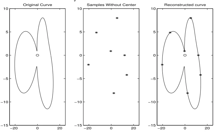
The above sampling procedure is sufficiently general to be applicable to a variety of curves. The sampling and unique reconstruction of a curveCis subject to the following conditions, which are, recall

• The admissible set from Definition 2.18 must be non-empty, i.e.,A_C ₆₌_∅.

• There must exist a pointγ0 ∈ AC, such that the corresponding polar parameterization ofC

is bandlimited.

The conditions we impose on a curve seem restrictive until we note that, unlike the1−Dcase, the proposed technique affords a reconstruction in spite of lack of complete samples and a fixed and unambiguous coordinate system.

The Figure 2.6 shows the result of applying the described technique to a curve, where we may also note that such an encoding ofγ0 is stable against random additive noise because of the

(44)

Figure 2.6 A curve is sampled and then perfectly reconstructed from the sampleswithoutusing any additional information.

−20 0 20 −15

−10 −5 0 5

10 Original Curve

−20 0 20 −15

−10 −5 0 5

10 Samples Without Center

−20 0 20 −15

−10 −5 0 5

(45)

2.4 General Applicability: Deviation From Model

As discussed in the beginning of this chapter, perfect reconstruction is impossible for arbi-trary signals in general, and curves in particular. Any reconstruction algorithm requires additional information about the nature of a signal. In many cases a signal is constrained to lie in a cer-tain functional space for the sampling theorem to be valid. The classical sampling theorem, for example, requires that a signal belong to the space of bandlimited functions.

Although class constraining, the above conditions, which a curve must satisfy to be a good candidate for sampling and exact reconstruction, are justifiable in light of the rather limited number of degrees of freedom imposed on an otherwise infinite dimensional space where our functions of interest live.

In the present context and for all practical purposes, where sampling of shapes is our main inter-est, a good approximation of curves will be perhaps no less important than an exact reconstruction. This in turn yields a number of interesting questions, such as:

• How close is the approximation to the original curve?

• Can we minimize the error of approximation?

(46)

may be written as

d(θ1, . . . , θN+1) = 0. (2.25)

We claimed earlier that it is always possible to find {θi}Ni=1+1 for a bandlimited curve, such

that (2.25) holds and where N matches the bandwidth. It is clearly seen that finite sampling and exact reconstruction are limited to bandlimited signals/curves. In the event that the curve is non-bandlimited, we may only seek to determine the samples, which will minimized(θ1, . . . , θN+1)

while optimizing the distance between the curve and its reconstructed approximation. Note that the previously described sampling procedure may be viewed as a particular case of this technique, which specializes to that above for the corresponding class of curves and for which the approxi-mation error is zero, and the two criteria optimization described next reduces to one.

2.4.1 Sampling By Optimized Approximation

Let us assume that we have a curveC, such thatA_C ₆₌_∅, and_γ₀ _∈A_C. Let_{r(θ), θ} _∈_[0,_2π]

be a polar parameterization, which is not necessarily bandlimited. Let N _∈ Nbe a fixed integer

number (for the sake of simplicity even). Towards formulating our generalized sampling define for each(N + 1)-tupleθ1, . . . , θN+1 ∈[0,2π]

d2(θ1, . . . , θN+1) =

N+1

X

i=1

r(θi) cos(θi)

!2

+

N+1

X

i=1

r(θi) sin(θi)

!2

, (2.26)

and

l2(θ1, . . . , θN+1) = 2π

Z

0

r(ϑ)−rˆθ1,...,θN+1(ϑ)

2 dϑ, (2.27)

whererˆθ1,...,θN+1(ϑ) is the reconstruction achieved by the samples defined atθ1, . . . , θN+1. In an

(47)

may achieve their minima at different points in an (N + 1)-dimensional space. We search for a so-called Pareto solution of the two-criteria optimization problem ([13]), which may be viewed as a point, from which any deviation may not decrease in one component without increasing in the other. For more details refer to [31]. DefineF : [0,2π]N+1 _→_R2 _{as follows}

F(θ1, . . . , θN+1) = d2(θ1, . . . , θN+1), l2(θ1, . . . , θN+1)

. (2.28)

Definition 2.22 A point(θ0

1, . . . , θN0+1)∈RN+1is called the Pareto optimal point ofF, if∀(θ1, . . . , θN+1)∈

RN+1 we have

      

d2_(θ

1, . . . , θN+1) ≤ d2 θ01, . . . , θ0N+1

l2_(θ

1, . . . , θN+1) ≤ l2 θ10, . . . , θN0+1

⇒

(θ1, . . . , θN+1) = (θ01, . . . , θ0N+1). (2.29)

Consider the case when the functionr(θ)is bandlimited, in the sense of Equation (2.22). There then exists according to Proposition 2.1 the corresponding number N + 1 and θ₁0, . . . , θ0_N₊₁ _∈ [0,2π],such that

      

d2 _θ0

1, . . . , θ0N+1

= 0, l2 θ0₁, . . . , θ_N0₊₁ = 0.

(2.30)

Because of the non-negativity of the functionsd2andl2, we conclude that the point θ₁0, . . . , θ_N0₊₁ is Pareto optimal, which also shows that our sampling technique described in the previous sections is a particular case of the multi-criteria optimization.

2.4.2 Implementation and Results

(48)

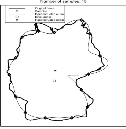
Figure 2.7 A good approximation of a map of Germany may be obtained from as few as 15 samples.

Number of samples: 15

Original curve Samples Reconstructed curve Initial origin Reconstructed origin

optimization problem (Pareto optimal point) have been proposed. Here we present the results ob-tained by using the steepest-descent method, which is while generally slow but proven to achieve the global optimal point. For the sake of space we defer the description of this method to [16] and only present the simulation results.

Figure 2.7 contains a silhouette of Germany. One can see that a reasonable approximation can be achieved using only 15 samples. A similar example is presented in Figure 2.8, where a very good reconstruction of a human kidney is made only from 7 samples. Finally, the shape of the human brain can be accurately encoded into 19 samples (Figure 2.9).

2.5 Further Extension: Sampling of Surfaces

(49)

Figure 2.8 A contour of a human kidney can be recovered from only 7 samples. Number of samples: 7

Original curve Samples Reconstructed curve Initial origin Reconstructed origin

Figure 2.9 A contour of a human brain can be recovered from only 19 samples. Number of samples: 19

(50)

1−Dsignal, a surface can be made into an image, by fixing spherical coordinates. Given that our interest focuses on2₋Dcurves, and that most of the results for surfaces are a simple generalization of the2₋Dcase, we forego any details and rather only state the results.

Definition 2.23 Suppose we have a surfaceS. If a pointγ0 ≡ (x0, y0, z0)is such that there exists

a functionr(θ, φ) : [0,2π]2 _→_R3_{, such that the surface}_S _{can be parameterized according to}

γ(θ, φ) = γ0+ r(θ, φ) cos(θ) cos(φ), r(θ, φ) cos(θ) sin(φ), r(θ, φ) sin(θ)

, (2.31)

where

φ, θ _∈[0,2π], γ(0, φ) =γ(2π, φ), γ(θ,0) =γ(θ,2π), (2.32)

then we callγ0 an admissible (spherical) center ofS.

Theorem 2.24 Let S be a smooth surface, (x0, y0, z0) ∈ R3, and ` - half-line starting from

(x0, y0, z0)and intersecting the image of S, set S, in at least two points. Then there exists

an-other half-line`t _{that also starts from}_(x

0, y0, z0)and is tangent toS.

Definition 2.25 Let S be a smooth surface and (x0, y0, z0) ∈ R3 be a point. Then this point is

called a regular admissible center if there exists no half-line` going from(x0, y0, z0)and tangent

toS. A collection of all regular admissible centers will be called the admissible set of a surfaceS and denotedA_S.

Theorem 2.26 LetS be a surface andA_S be its admissible set. ThenA_Sis convex, i.e.,

γ1, γ2 ∈AC

⇒[γ1, γ2]⊂AC

(51)

where

[γ1, γ2] =

αγ1+ (1−α)γ2 |α∈[0,1] . (2.34)

Theorem 2.27 Suppose that we have a curveS andγ0 ∈AS. Letr(θ, φ)be a spherical

represen-tation ofScentered atγ0. Then ifr(θ, φ)is bandlimited, so that∃M, N ∈N, such that

r(θ, φ) =

M/2

X

m=−M/2

N/2

X

n=−N/2

cm,neiθn·eiφm, (2.35)

thenr(θ, φ)can be reconstructed from any samples so long as their number is sufficient.

Proposition 2.3 LetS be a curve andγ0 ∈ AS. Without loss of generality we will assume that

γ0 = (0,0,0). Suppose thatr(θ, φ), (θ, φ)∈[0,2π]2is a corresponding spherical parameterization

ofS. Then ifr(θ, φ)is bandlimited, then we can always choose sampling grid(θi, φj) in such a

way that

X

i,j

r(θi, φj) cos(θi) cos(φj), r(θi, φj) cos(θi) sin(φj), r(θi, φj) sin(θi)

= (0,0,0). (2.36)

Proposition 2.4 LetS be a curve. AssumeA_S ₆₌ _∅, and _γ₀ _≡ _(x₀_{, y}₀_{, z}₀₎ _∈ A_S. Suppose that

r(θ, φ)is a spherical parameterization ofScentered atγ0. Ifr(θ, φ)is bandlimited, then there exist

distinct points(θi, φj)such that the curveS is uniquely defined by the corresponding samples of

(52)

2.6 Chapter Summary

Sampling of curves and surfaces is as important for a number of applications as sampling of1₋

Dor2−Dsignals. It may help to compress certain images more efficiently, than other techniques that work with an entire image. Sampling also helps to provide us with shape landmarks, which are an essential tool for shape analysis and computer vision.

It was shown that a direct attempt to sample a curve encounters the difficulty, which is not topical for a signal or an image, namely that of finding a functional representation of the curve. Making sure that a curve will always have a parametrization of a prescribed type requires imposing constraints on the nature of the curve. It was demonstrated that for the case of polar parametrization such constraints could be found and efficient class identification numerical procedures could be implemented.

It was further discussed that unlike the1₋Dcase, samples of a curve are meaningless unless they carry information about a coordinate system in which the curve had been parameterized. We used the flexibility in choosing positions of sampling points when dealing with a1₋Dbandlimited signal to incorporate the information about the polar center into the samples of a curve. The resulting procedure yielded a technique allowing us to reconstruct a curve from its samples without any additional information.

(53)

Chapter 3 On a New Implementation of Simulated Annealing and Its

Appli-cation to Signal and Image Filtering

3.1 Introduction

Many tasks in signal and image processing such as filtering, segmentation, pattern recognition and other applications may be posed in the context of an optimization problem. Given an initial or observed dataf0, to any signalfwe associate a certain valueHf0(f). The functionalf →Hf0(f),

which assigns a number to a signal, is generally referred to as the signal energy or cost. The energy (cost) of a signal is thus a function of the signal and the observed data. Our goal is then to minimize this cost, i.e. find a signal_fˆ_{with the lowest energy. Mathematically, we can write it as}

ˆ

f = arg min

f H_f

0(f). (3.1)

The solution to the problem (3.1) then becomes the output of a system that is being designed. The problem of finding a cost functionalH suitable for a particular application is challenging.

(54)

0 1 2 3 4 5 6 −3

−2 −1 0 1 2 3

t

f(t)

Clean signal

0 1 2 3 4 5 6

−3 −2 −1 0 1 2 3

t

f(t) + n(t)

Noisy signal

Figure 3.1 Example of a clean signal and the same signal corrupted by additive Gaussian noise.

A general approach to such a problem is to search for a signal which is close to the observation with all irregularities believed to be due to the noise factored out. A functional destined for filtering would therefore require two components. One would penalize large deviations from the observed data, and the other one would penalize signal abnormalities that are rather attributed to the noise than to the clean signal, i.e. impose some regularity on the signal.

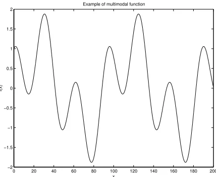
The complex structure of the functional almost invariably results in the latter being multi-modal, i.e. having more than one local extremum (see Figure 3.2). A typical gradient descent method which is used to search for a local minimum thus becomes suboptimal, and additional effort is required to either improve on the extremum or in the best case converge to a global extremum.

(55)

0 20 40 60 80 100 120 140 160 180 200 −2

−1.5 −1 −0.5 0 0.5 1 1.5 2

x

f(x)

Example of multimodal function

(56)

Indisputable advantages of many simulated annealing based algorithms pertain to their ability accommodate complex cost functionals with large number of degrees of freedom in a straightfor-ward and easy-to-implement manner. In addition, in many cases an algorithm from this class may be proven to be optimal in the sense of convergence to a global minimum.

On the other hand, straightforward implementations of simulated annealing suffer from serious shortcomings, perhaps the most important of which is their low rate of convergence. Many algo-rithms have been proposed in the literature in order to address this problem and potentially achieve a superior performance at a cost of greatly complicating the stochastic component of the algorithm. Our goal in this chapter is in this direction by proposing a modification of a classical simulated an-nealing scheme, to attain a faster descent while maintaining the simplicity of the original idea and its implementation.

(57)

in an extremely large time period before the particle finds a better stable state, i.e. another local minimum with smaller energy.

A step in the direction of dealing with this problem was the well-known fast simulated anneal-ing or the Cauchy machine proposed by Szu, whose idea was to make the tails of the distribution of jump sizes heavier, hence allowing occasional large jumps, which would help exploring areas far from the current position of the particle much faster. This approach unfortunately only partially addresses the scale problem described above. The technique uniformly fails at fine scales, as a particle may be moved by a large jump with no regards to whether a better local minimum is in proximity. It has also been reported that the Cauchy machine does not converge in theory, which limits its practical importance.

Our approach is based on systematically exploring all scales while maintaining the simplic-ity of implementation. In lieu of keeping the temperature constant, we propose to vary it non-monotonously by first exploring the immediate neighborhood of the current local minimum and then by proceeding to progressively increase its size. While much of the theoretical analysis is left as part of future work, experimental results show that a significant improvement in achieving the lowest possible energy state within a minimal time.

(58)

the region where the global minimum is most likely to be found, results in further improvement of the search algorithm. Some initial states, due to their close proximity to the global minimum, faster converge to the optimal state.

This chapter is organized as follows. Section 3.2 provides the general background about stochastic optimization in general, and simulated annealing in particular. Section 3.3 is devoted to the description of the newly proposed algorithm based on using adaptive temperature to obtain a fast implementation of simulated annealing. Section 3.4 discusses the evolution of perturbations of the original signal as opposed to the original signal, which yields better minimization results. A summary of the chapter is given in Section 3.5.

3.2 Simulated Annealing

Consider a problem of finding the global minimum ofH_f

0(f), wheref0 ∈R

d _{for some integer}

d_≥1, andH_f

0(·) :R

d _→_R_{. In other words, find}_fˆ_∈_Rd_{, such that}

ˆ

f = arg min

f∈Rd H_f

0(f). (3.2)

Heref, f0 are multidimensional vectors, which represent discrete signals or images; f0 being the

observed data.

The problem (3.2) can be solved by introducing an interactive diffusion process{f(t)}t≥0, such

that∀d _≥0, f(t) _∈ Rd. Let_σ _: R _→Rbe a 1D function, which we will call the “temperature”.

Consider the following stochastic differential equation with the initial condition

df(t) =−∇fHf0(f)dt+σ(t)dw(t), (3.3a)

(59)

where∇f denotes the gradientw(t)is ad-dimensional Brownian motion. The right hand side of

the equation (3.3a) consists of two terms. The first one is deterministic and represents nothing but the famous gradient descent, while the second one is diffusive and called for to de-trap the process

f(t)from local minima of the functionalH_f

0(·).

The equation (3.3a) is by definition equivalent to the following integral representation for the processf(t).

fi(t) =f0,i+ t Z 0 − ∂ ∂fi H_f

0 f(u)

du+σ(t)

t

Z

0

dwi(u), i= 1, . . . , d, (3.4)

where

f(t)_≡ f1(t), . . . , fd(t)

T

, f0 ≡ f1,0, . . . , fd,0

T

, w(t)_≡ w1(t), . . . , wd(t)

T

.

Considering Equation (3.3a) with

σ(t) = p σ0

log(t+ 1), (3.5)

whereσ0 is a fixed constant, yields the convergence of the stochastic differential equation (3.3) to

the solution_{f, which is the global minimum of}ˆ H_f

0(·), i.e.

H_f

0

ˆ

f= min

f∈Rd H_f

0(f). (3.6)

3.2.1 Discrete Approximation of the Filtering Scheme

The implementation of the above scheme entails discretization of the above equations. To-wards that end, we construct a discrete time process {g(n)_}n=1,2,..., which will approximate the

(60)

Consider a fixed interval(0, t)and letδ = _N1, whereN is a (large) integer number. Define

τn =nδ, n = 1, . . . , N. (3.7)

Then the process{g(n)}may be constructed using the following iterative scheme,

gi(n+ 1) =gi(n)−

∂ ∂gi

H_f

0 g(n)

·δ+σ(t)· w(τn+1)−w(τn)

, (3.8a)

g(0) =f0. (3.8b)

The diffusion (3.3) is approximated by the discrete process (3.8) as spelled out by the following theorem.

Theorem 3.1 (Descombes, Zhizhina) Under certain very mild assumptions on the functionalH_f

0(·),

the approximation process (3.8) strongly converges to the diffusion (3.3) with order 1

2. More

pre-cisely,

∀t _≥0, max

i=1,...,d

Eh_f_i_(t)₋_g_i_(n_t₎ i

≤C(t)√δ. (3.9)

Theorem (3.1) assures that for δ small enough, the behavior of the discrete approximation

{g(n)_}is indistinguishable from its continuous counterpart _{f(t)_}. Thus we should expect from the discrete process, the same filtering properties that are attributed to the continuous diffusion.

(61)

its discretized version is slow due to the slow decay of the diffusion coefficient. In practice, this tantamount to introducing a Gaussian component with virtually constant variance at each iteration of (3.8), which, of course, adversely affects the convergence of the algorithm within any reasonable computational time.

We next keep the difference equation (3.8) as a guide when constructing a framework with enhanced convergence properties.

3.3 Adaptive temperature

Consider a particular case of the optimization problem in Equation (3.2) when d = 1. Here we will use the following notation. Let F : R _→ R be a function defined on the real line and

sufficiently smooth. Our goal is to find the global minimumuˆofF(_·), i.e.

ˆ

u= arg min

u∈RF(u). (3.10)

The simulated annealing technique presented above yields the following stochastic differential equation to solve Equation (3.10).

du(t) =₋F0 u(t)dt+σ(t)dw(t), (3.11a) wherew(t) is a 1D Wiener process. The discrete approximation of equation (3.11a) can then be written as follows:

un+1=−F0(un)·δ+σn·wn, (3.11b)

where{wn}n=1,2,...are independent identically distributed Gaussian random variables

(62)

and the temperaturesσn, n = 1,2, . . .are defined as

σn=

1 p

log(nδ+ 1).

It is apparent from Equation (3.11b) that a slow decay of the coefficientsσnresults in

introduc-ing Gaussian noise of virtually constant variance at each step of iteration. It is convenient to think of the time intervalδ as determining the scale at which the search is being carried out. Whenδis fixed and the temperatureσn varies slowly, the search process takes place at essentially one fixed

scale. If local minima are closely clustered in relation to a typical jump size of a diffusing particle, then many including those with lower energies will be overlooked for an extended period of time. On the other hand, if the distance between extrema is too large, then the diffusion energy is too small to allow a fast exploration of the functional and hence an efficient localization of new ex-trema, i.e. the particle is trapped in one mode for too long. The following proposition provides the exact relationship between the inter-local minima distance and the scale of the discrete diffusion.

Proposition 3.1 Let F : R _→ R be a 1D function, and _α _∈ R a fixed real constant. Define

G:R_→Rby

∀x_∈R_{, G(x) =}_F_(αx). (3.12)

Then the discrete procedure of minimization of the function Gon the scaleδ is equivalent to minimizing the functionF at the scaleα2δ.

Proof. The minimization evolution for the functionGis of the form