Abstract
SHARPE, JOHN PHILLIP. Particulate Generation During Disruption Simulation on the SIRENS High Heat Flux Facility. (Under the direction of Professor Mohamed Bourham and Professor John G. Gilligan.)
Particulate Generation During Disruption Simulation
on the SIRENS High Heat Flux Facility
by
John Phillip Sharpe
A thesis submitted to the Graduate Faculty of North Carolina State University
in partial fulfillment of the requirements for the Degree of
Doctor of Philosophy
Nuclear Engineering
Raleigh, North Carolina
2000
Approved By:
_________________________________ Dr. Mohamed A. Bourham, Chair of Advisory Committee
_________________________________ Dr. Kuruvilla Verghese
________________________________ Dr. John G. Gilligan,
Co-chair of Advisory Committee
________________________________ Dr. Christopher Roland
Dedication
Biography
Acknowledgements
Table of Contents
List of Figures ...viii
List of Tables ...xv
1. Introduction...1
2. Research Review...4
2.1 Particulate Collected from Existing Tokamaks ...4
2.2 Particulate Collected from Plasma Guns ...5
2.3 Particulate Collected from Laser Experiments ...5
3. The SIRENS Facility: Application to Particulate Study...7
3.1 Overview of ET Gun Operation...7
3.2 SIRENS Specifications ...8
3.3 Modifications for Particulate Study ...11
3.4 Characterization of the Particulate...13
3.4.1 Condensate Collection by Capture Buttons ...13
3.4.2 Observation of Particulate...17
3.4.3 Image Analysis and Generation of Size Distributions...20
3.5 Scoping Test Results...24
3.5.1 Shot S710 ...24
3.5.2 Shots S712 and S713 ...25
3.5.3 Shot S715 ...31
4. Experiment Results: Metals Tests...37
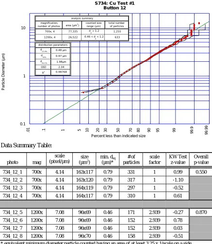
4.1 Copper Results ...37
4.1.1 Test 1: S734 ...37
4.1.2 Test 2: S737 ...50
4.2 SS316 Results ...62
4.2.1 Test 1: S735 ...63
4.2.2 Test 2: S738 ...74
4.3 Tungsten Results...83
4.3.1 Test 1: S736 ...84
4.3.2 Test 2: S739 ...94
4.4 Aluminum Results ...101
4.4.1 Test 1: S744 ...102
4.4.2 Test 2: S745 ...109
5. Experiment Results: Carbon and Mixed-Material Tests...113
5.1 Carbon Results ...114
5.1.2 Graphite Tests: S763 and S764...127
5.2 Carbon/Copper Results ...142
5.2.1 Short Configuration: S765 ...143
5.2.2 Segmented Configuration: S769 ...151
5.3 Carbon/SS316 Results ...160
5.3.1 Short Configuration: S766 ...161
5.3.2 Segmented Configuration: S770 ...171
5.4 Carbon/Tungsten Results: S767...179
5.5 Carbon/Aluminum Results: S768 ...188
5.6. Summary of Mixed-Materials Tests ...198
6. Models Developed for Experiment Simulation ...201
6.1 Plasma/Fluids Model ...201
6.1.1. Mass Conservation...204
6.1.2 Energy Conservation...214
6.1.2.1 Electron Energy Equation ...214
6.1.2.2. Ion Energy Equation ...215
6.1.2.3. Neutral Energy Equation...218
6.1.3. Momentum Conservation...219
6.1.3.1 Electron Momentum Equation...220
6.1.3.2. Ion Momentum Equation ...221
6.1.3.3. Neutral Momentum Equation ...223
6.1.4. Solution Strategy...226
6.1.5. Benchmark Test: Plasma Models...230
6.1.5.1. Gun/Barrel Configuration ...230
6.1.5.2. Gun/Chamber Configuration ...236
6.1.5.3. Comparison of Results from Other Models (ODIN and TITAN) ...240
6.1.6. Benchmark Test: Shock Tube Transient...243
6.1.7. Benchmark Test: Nozzle Flow Model ...252
6.2 Particulate Growth and Transport Model ...259
6.2.1 Aerosol General Dynamic Equation (GDE) ...259
6.2.1.1. Homogeneous Nucleation...261
6.2.1.2. Heterogeneous Nucleation/Growth...262
6.2.1.3. Coagulation ...265
6.2.2. Discretized Aerosol GDE ...267
6.2.3. Benchmark Test: Coagulation...270
6.2.4. Benchmark Test: Condensation Growth...272
6.2.5. Model Test: Nucleation and Growth without Flow ...289
7. Simulation of SIRENS Particulate Production Experiments ...297
7.1. Copper Test Simulation ...298
7.2. Iron/SS316 Test Simulation...327
7.3. Tungsten Test Simulation ...337
7.4. Aluminum Test Simulation...346
8. Summary and Recommendations ...355
8.1. Contributions of the Experiment Campaign ...355
8.2. Contributions of the Modeling Effort ...357
8.3. Recommendations for Future Investigation...359
References...361
Appendices: Appendix A Derivation of the Plasma/Fluids Conservation Equations ...367
Appendix B Listing of the TOPGUN Computer Code ...382
Appendix C Listing of the TOPAERO Computer Code ...408
List of Figures
Chapter 3:
3.1. Electrothermal source configuration of SIRENS for nominal operation. 8 3.2. Layout of SIRENS, including various diagnostic tools for standard operation. 9
3.3. Pulsed-power network (PPN) for energizing SIRENS. 10
3.4. Modified SIRENS source section. 14
3.5. Modified SIRENS facility with the source section and expansion chamber. 14
3.6. Schematic of collection button distribution. 15
3.7. SEM micrographs from button 11 of scoping test S715. 19
3.8. Optical microscope photographs of button 10 from scoping test S715. 19 3.9. Schematic depiction of the size distribution construction technique. 21 3.10. Log probability distribution constructed by NCSU and INEEL for DIII-D
Q1DV dust. 23
3.11. S713 current and voltage traces. 26
3.12. SEM micrographs from S712 and S713. 28
3.13. Count distributions for Shot S712. 28
3.14. Count distributions for Shot S713. 30
3.15. Axial mass deposition on collection buttons for S712 and S713. 31
3.16. Representative SEM micrographs from S715. 33
3.17. Particle size distribution from S715. 34
3.18. Particle size distribution from S715 Button 10, SEM vs. optical microscope. 35
3.19. Axial mass deposition on collection buttons for S715. 36
3.20. EDX images from button S715 Button 11. 36
Chapter 4:
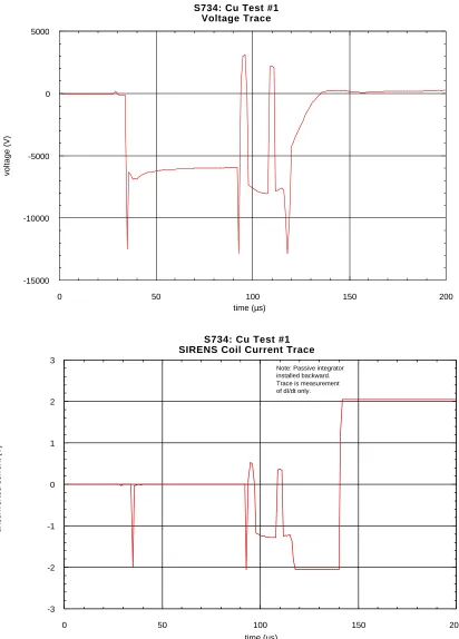
4.1. Cu Test #1 voltage and current traces. 41
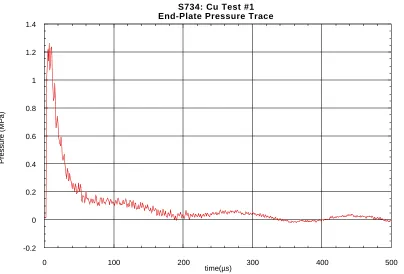
4.2. Cu Test #1 end-plate P transducer trace. 42
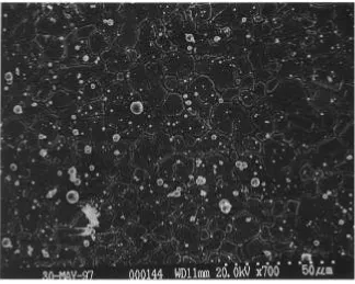
4.3. SEM images from Cu Test #1 showing the distinct substrate grain
boundaries which tend to interfere with image analysis. 43
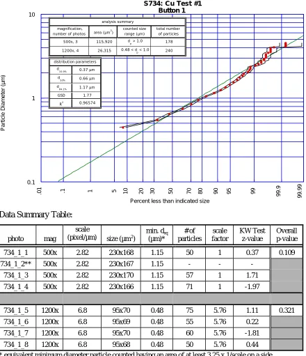
4.4 Cu Test #1, Button 1 particle size distribution. 44
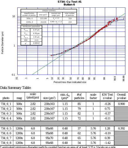
4.5. Cu Test #1, Button 6 particle size distribution. 45
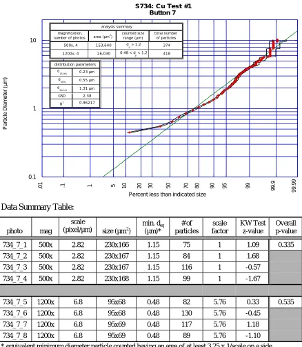
4.6. Cu Test #1, Button 7 particle size distribution. 46
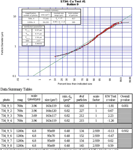
4.7. Cu Test #1, Button 9 particle size distribution. 47
4.8. Cu Test #1, Button 12 particle size distribution. 48
4.9. Cu Test #1, Button 14 particle size distribution. 49
4.10. Cu Test #2 voltage and current traces. 52
4.11. Cu Test #2 source and end-plate P transducer traces. 53
4.12. Cu Test #2, Button 1 particle size distribution. 54
4.13. Cu Test #2, Button 6 particle size distribution. 55
4.14. Cu Test #2, Button 7 particle size distribution. 56
4.15. Cu Test #2, Button 9 particle size distribution. 57
4.16. Cu Test #2, Button 12 particle size distribution. 58
4.17. Cu Test #2, Button 14 particle size distribution. 59
4.18. EDXA spectra from 2 different regions on Button 9 in Cu Test #2. 60
4.20. SS316 Test #1 end-plate P transducer trace. 66
4.21. SS316 Test #1, Button 1 particle size distribution. 67
4.22. SS316 Test #1, Button 6 particle size distribution. 68
4.23. SS316 Test #1, Button 7 particle size distribution. 69
4.24. SS316 Test #1, Button 9 particle size distribution. 70
4.25. SS316 Test #1, Button 12 particle size distribution. 71
4.26. SS316 Test #1, Button 14 particle size distribution. 72
4.27. Representative SEM images from Button 7, SS316 Test #1. 73
4.28. SS316 Test #2 voltage and current traces. 75
4.29. SS316 Test #2 end-plate P transducer trace. 76
4.30. SS316 Test #2, Button 1 particle size distribution. 77
4.31. SS316 Test #2, Button 6 particle size distribution. 78
4.32. SS316 Test #2, Button 7 particle size distribution. 79
4.33. SS316 Test #2, Button 9 particle size distribution. 80
4.34. SS316 Test #2, Button 12 particle size distribution. 81
4.35. SS316 Test #2, Button 14 particle size distribution. 82
4.36. W Test #1 voltage and current traces. 85
4.37. W Test #1 end-plate P transducer trace. 86
4.38. W Test #1, Button 1 particle size distribution. 87
4.39. W Test #1, Button 6 particle size distribution. 88
4.40. W Test #1, Button 7 particle size distribution. 89
4.41. W Test #1, Button 9 particle size distribution. 90
4.42. W Test #1, Button 12 particle size distribution. 91
4.43. W Test #1, Button 14 particle size distribution. 92
4.44. Representative SEM images from W Test #1, Button 12. 93
4.45. W Test #2 voltage and current traces. 96
4.46. W Test #2 end-plate P transducer trace. 97
4.47. W Test #2, Button 1 particle size distribution. 98
4.48. W Test #2, Button 6 particle size distribution. 99
4.49. W Test #2, Button 7 particle size distribution. 100
4.50. Al Test #1 voltage and current traces. 103
4.51. Al Test #1, Button 3 particle size distribution. 105
4.52. Al Test #1, Button 7 particle size distribution. 106
4.53. Al Test #1, Button 9 particle size distribution. 107
4.54. Representative SEM images from Al Test #1, Button 7. 108
4.55. Al Test #2, Button 3 particle size distribution. 110
4.56. Al Test #2, Button 7 particle size distribution. 111
4.57. Al Test #2, Button 9 particle size distribution. 112
Chapter 5:
5.1. Carbon / metal mixture test sleeve configurations. 114
5.2. Voltage and current traces for both Lexan tests. 118
5.3. Power and energy traces for Lexan test S760. 119
5.8. Lexan test 2 (S761) button 1 particle size distribution. 124 5.9. Lexan test 2 (S761) button 3 particle size distribution. 125 5.10. Lexan test 2 (S761) button 9 particle size distribution. 126 5.11. Optimal source section configuration for carbon tests S763 and S764. 128 5.12. Voltage and current traces for graphite carbon tests S763 and S764. 129 5.13. Power and energy traces for graphite carbon tests S763 and S764. 130 5.14. Representative SEM micrographs of button 3 from UTR-22 graphite
test S763. 131
5.15. Representative SEM micrographs of button 3 from ATJ graphite test S764. 132 5.16. UTR-22 graphite test (S763) button 1 particle size distribution. 134 5.17. UTR-22 graphite test (S763) button 3 particle size distribution. 135 5.18. UTR-22 graphite test (S763) button 9 particle size distribution. 136 5.19. ATJ graphite test (S764) button 1 particle size distribution. 137 5.20. ATJ graphite test (S764) button 3 particle size distribution. 138 5.21. ATJ graphite test (S764) button 5 particle size distribution. 139 5.22. ATJ graphite test (S764) button 7 particle size distribution. 140 5.23. ATJ graphite test (S764) button 9 particle size distribution. 141 5.24. Voltage and current traces for C/Cu short test (S765). 144
5.25. Power and energy traces for C/Cu short test (S765). 144
5.26. Representative SEM micrographs from button 3 of S765. 145
5.27. EDXA mapping results of a button 2 region containing a Cu particle. 147 5.28. Carbon / Copper short test (S765) button 1 particle size distribution. 148 5.29. Carbon / Copper short test (S765) button 3 particle size distribution. 149 5.30. Carbon / Copper short test (S765) button 9 particle size distribution. 150 5.31. Voltage and current traces for C/Cu segmented test (S769). 152 5.32. Power and energy traces for C/Cu segmented test (S769). 152
5.33. Representative SEM micrographs from button 2 of S769. 153
5.34. EDXA mapping results of a button 2 region containing a Cu particle. 155 5.35. Optical spectra of the expanding vapor from the S769 source section. 155 5.36. Carbon / Copper segmented test (S769) button 1 particle size distribution. 156 5.37. Carbon / Copper segmented test (S769) button 2 particle size distribution. 157 5.38. Carbon / Copper segmented test (S769) button 3 particle size distribution. 158 5.39. Carbon / Copper segmented test (S769) button 17 particle size distribution. 159 5.40. Voltage and current traces for C/SS316 short test (S766). 162 5.41. Power and energy traces for C/SS316 short test (S766). 162
5.42. Representative SEM micrographs from button 3 of S765. 163
5.43. EDXA mapping results of a region on button 2 containing SS316 particles. 165 5.44. Carbon / SS316 short test (S766) button 1 particle size distribution. 166 5.45. Carbon / SS316 short test (S766) button 2 particle size distribution. 167 5.46. Carbon / SS316 short test (S766) button 3 particle size distribution. 168 5.47. Carbon / SS316 short test (S766) button 5 particle size distribution. 169 5.48. Carbon / SS316 short test (S766) button 9 particle size distribution. 170 5.49. Voltage and current traces for C/SS316 segmented test (S770). 172 5.50. Power and energy traces for C/SS316 segmented test (S770). 172
5.51. Representative SEM micrographs from button 3 of S770. 173
5.53. Optical spectra of the expanding vapor from the S770 source section. 175 5.54. Carbon / SS316 segmented test (S770) button 1 particle size distribution. 176 5.55. Carbon / SS316 segmented test (S770) button 3 particle size distribution. 177 5.56. Carbon / SS316 segmented test (S770) button 9 particle size distribution. 178
5.57. Source section configuration used in C/W test S767. 179
5.58. Voltage and current traces for carbon / tungsten test S767. 181 5.59. Power and energy traces for carbon / tungsten test S767. 181
5.60. Representative SEM micrographs from button 2 of S767. 182
5.61. Carbon / Tungsten test (S767) button 1 particle size distribution. 184 5.62. Carbon / Tungsten test (S767) button 2 particle size distribution. 185 5.63. Carbon / Tungsten test (S767) button 5 particle size distribution. 186 5.64. Carbon / Tungsten test (S767) button 9 particle size distribution. 187 5.65. Voltage and current traces for Lexan carbon / aluminum test S768. 190 5.66. Power and energy traces for Lexan carbon / aluminum test S768. 190
5.67. Representative SEM micrographs from button 2 of S768. 191
5.68. EDXA mapping results of a button 2 region containing Al particles. 192 5.69. Carbon / Aluminum test (S768) button 1 particle size distribution. 193 5.70. Carbon / Aluminum test (S768) button 2 particle size distribution. 194 5.71. Carbon / Aluminum test (S768) button 3 particle size distribution. 195 5.72. Carbon / Aluminum test (S768) button 5 particle size distribution. 196 5.73. Carbon / Aluminum test (S768) button 9 particle size distribution. 197
Chapter 6:
6.1. Model configuration of the experiment source section and expansion chamber.202
6.2. Axial nodalization for the plasma/fluid model. 202
6.3. Equilibrium effective charge state and densities for carbon. 211 6.4(a). Equilibrium effective charge state and densities for copper. 212 6.4(b). Effective charge state for copper given by Saha and conservation models. 213
6.5(a). Flow chart for solving plasma/fluids model. 227
6.5(b). Inner loop flow chart for updating temperatures and densities. 228
6.6. Pressure profiles for gun/barrel simulation. 232
6.7. Neutral velocity profile for gun/barrel simulation. 233
6.8. Predicted vs. measured discharge voltage for gun/barrel simulation. 233 6.9. Neutral temperature profiles for gun/barrel simulation. 234 6.10. Temperature profiles at 35 µs for gun/barrel simulation. 234 6.11. Temperature profiles at 70 µs for gun/barrel simulation. 235 6.12. Temperature profiles at 100 µs for gun/barrel simulation. 235 6.13. Temperature profiles at 200 µs for gun/barrel simulation. 236
6.14. Geometry for the gun/chamber configuration. 237
6.15. Source section pressure profiles for the gun/chamber configuration. 238 6.16. Chamber section pressure profiles for the gun/chamber configuration. 238 6.17. Vapor velocity profiles for the gun/chamber configuration. 239 6.18. Neutral temperature profiles for the gun/chamber configuration. 239 6.19. S776 gun average pressure from TOPGUN, ODIN, and TITAN. 241
6.21. S776 gun average temperature from TOPGUN, ODIN, and TITAN. 242 6.22. S776 gun average plasma density from TOPGUN, ODIN, and TITAN. 243
6.23. Mach number profiles for the shock-tube test. 246
6.24. Temperature profiles for the shock-tube test. 248
6.25. Pressure profiles for the shock-tube test. 250
6.26. Test nozzle geometric configuration. 254
6.27. Mach number profile for sub-sonic nozzle. 254
6.28. Pressure profile for sub-sonic nozzle. 255
6.29. Temperature profile for sub-sonic nozzle. 255
6.30. Mach number profile for super-sonic nozzle, internal shock. 256 6.31. Pressure profile for super-sonic nozzle, internal shock. 256 6.32. Temperature profile super-sonic nozzle, internal shock. 257 6.33. Mach number profile for super-sonic nozzle, external shock. 257 6.34. Pressure profile for super-sonic nozzle, external shock. 258 6.35. Temperature profile super-sonic nozzle, external shock. 258 6.36. Homogeneous nucleation results for copper (small scale). 263 6.37. Homogeneous nucleation results for copper (large scale). 263
6.38. Homogeneous nucleation results for tungsten. 264
6.39. Homogeneous nucleation results for aluminum. 264
6.40. Analytical and Numerical Solutions for the Coagulation-Only Aerosol GDE. 272
6.41. Condensation-only Test: Uniform Distribution, K=50. 276
6.42. Condensation-only Test: Uniform Distribution, K=50 (linear count scale). 277
6.43. Condensation-only Test: Uniform Distribution, K=200. 278
6.44. Condensation-only Test: Uniform Distribution, K=200 (linear count scale). 279
6.45. Absolute RMS error for initial uniform distribution. 280
6.46. Condensation-only Test: Gamma Distribution, K=50. 280
6.47. Condensation-only Test: Gamma Distribution, K=50 (linear count scale). 282
6.48. Condensation-only Test: Gamma Distribution, K=200. 282
6.49. Condensation-only Test: Gamma Distribution, K=200 (linear count scale). 284
6.50. Absolute RMS error for initial gamma distribution. 284
6.51. Condensation-only Test: Log-normal Distribution, K=50. 285 6.52. Condensation-only Test: Log-normal Distribution, K=50 (linear count scale). 286 6.53. Condensation-only Test: Log-normal Distribution, K=200. 287 6.54. Condensation-only Test: Log-normal Distribution, K=200 (linear count scale).288 6.55. Absolute RMS error for initial lognormal distribution. 289 6.56. Saturation ration versus time for the model test case. 291 6.57. Vapor mass density and total particle mass density for the model test case. 291 6.58. Particle size distribution at various times for the model test case. 292
6.59. Flow diagram of coupled models solution strategy. 293
Chapter 7:
7.6. Total mass ablated from source section in the Cu test simulation. 308 7.7. Average species temperatures during the discharge of the Cu test simulation. 308
7.8. Temperature profiles for the Cu test simulation. 309
7.9. Chamber region-averaged temperature traces for the Cu test simulation. 310
7.10. Gun-exit pressure trace for Cu test simulation. 312
7.11. Pressure profiles for the Cu test simulation. 312
7.12. Chamber region-averaged pressure traces for the Cu test simulation. 314
7.13. Gun-exit velocity trace for the Cu test simulation. 316
7.14. Velocity profiles for the Cu test simulation. 316
7.15. Chamber region-averaged velocity traces for the Cu test simulation. 317
7.16. Saturation ratio profiles for the Cu test simulation. 319
7.17. Chamber region-averaged saturation ratio traces for the Cu test simulation. 320 7.18. Total vapor and aerosol mass traces for the Cu test simulation. 322 7.19. Chamber region-averaged aerosol concentration for the Cu test simulation. 322 7.20. Regional particle size distributions for the Cu test simulation. 323 7.21. Predicted and measured particle size distributions for the Cu test simulation. 325 7.22. Predicted and measured voltage for the Fe test simulation. 330 7.23. Average species temperatures during the discharge of the Fe test simulation. 330
7.24. Temperature profiles for the Fe test simulation. 331
7.25. Pressure profiles for the Fe test simulation. 332
7.26. Velocity profiles for the Fe test simulation. 333
7.27. Saturation ratio profiles for the Fe test simulation. 334
7.28. Total vapor and aerosol mass traces for the Fe test simulation. 334 7.29. Chamber region-averaged aerosol concentration for the Fe test simulation. 335 7.30. Predicted and measured particle size distributions for the Fe test simulation. 335 7.31. Predicted and measured voltage for the W test simulation. 339 7.32. Average species temperatures during the discharge of the W test simulation. 339
7.33. Temperature profiles for the W test simulation. 340
7.34. Pressure profiles for the W test simulation. 341
7.35. Velocity profiles for the W test simulation. 342
7.36. Saturation ratio profiles for the W test simulation. 343
7.37. Total vapor and aerosol mass traces for the W test simulation. 343 7.38. Chamber region-averaged aerosol concentration for the W test simulation. 344 7.39. Predicted and measured particle size distributions for the W test simulation. 344 7.40. Predicted and measured voltage for the Al test simulation. 348 7.41. Average species temperatures during the discharge of the Al test simulation. 348
7.42. Temperature profiles for the Al test simulation. 349
7.43. Pressure profiles for the Al test simulation. 350
7.44. Velocity profiles for the Al test simulation. 351
Appendix D:
D.1. Saturation vapor pressure for Al, Cu, Fe, and W. 418
D.2. Ionization and recombination reaction rates for Al. 419
D.3. Radiation cooling rate for Al. 420
D.4. Ionization and recombination reaction rates for C. 421
D.5. Radiation cooling rate for C. 422
D.6. Ionization and recombination reaction rates for Cu. 423
D.7. Radiation cooling rate for Cu. 424
D.8. Ionization and recombination reaction rates for Fe. 425
D.9. Radiation cooling rate for Fe. 426
D.10. Ionization and recombination reaction rates for W. 427
List of Tables
Chapter 3:
3.1. SIRENS Operational Characteristics. 9
3.2. Available Diagnostics on SIRENS. 9
3.3. Comparison of relevant ITER and SIRENS parameters. 12
3.4. Tabulated button distribution for the experimental configuration. 15
3.5. Control button analysis. 17
3.6. Scale Factors for the optical microscope and the SEM microscope. 22 3.7. Comparison of NCSU analysis verses INEEL analysis for DIII-D Q1DV. 22
3.8. Scoping Shots Summary. 24
3.9. Summary of Particle Size Distribution Data for S712 and S713. 27
3.10. Summary of Particle Size Distribution Data for S715. 33
Chapter 4:
4.1. Cu tests comparison summary. 38
4.2. Cu Test #1: S734 mass measurements. 42
4.3. Cu Test #2: S737 mass measurements. 53
4.4. SS316 tests comparison summary. 62
4.5. SS316 Test #1: S735 mass measurements. 66
4.6. SS316 Test #1: S738 mass measurements. 76
4.7. W tests comparison summary. 83
4.8. W Test #1: S736 mass measurements. 86
4.9. W Test #2: S739 mass measurements. 97
4.10. Al tests comparison summary. 101
4.11. Al Test #1: S734 mass measurements. 104
4.12. Al Test #2: S745 mass measurements. 109
Chapter 5:
5.1. Carbon tests comparison summary. 115
5.2. Lexan tests mass measurements. 119
5.3. Graphite carbon test mass measurements. 128
5.4. Carbon / Copper tests comparison summary. 142
5.5. Carbon / Copper short test mass measurements. 145
5.6. Carbon / Copper segmented test mass measurements. 153
5.7. Carbon / SS316 tests comparison summary. 160
5.8. Carbon / SS316 short test mass measurements. 163
5.9. Carbon / SS316 segmented test mass measurements. 173
5.10. Carbon / Tungsten test results summary. 179
5.11. Lexan carbon / tungsten test mass measurements. 182
5.12. Carbon / Aluminum test results summary. 188
5.13. Lexan carbon / aluminum test mass measurements. 191
5.14. Summary test data and particle size distribution parameters. 199
Chapter 6:
Chapter 7:
7.1. Summary of Cu test simulation and Cu experiment measurements. 305 7.2. Summary of Fe test simulation and SS316 experiment measurements. 327 7.3. Summary of W test simulation and W experiment measurements. 337 7.4. Summary of Al test simulation and Al experiment measurements. 346
Appendix D:
Particulate Generation During Disruption Simulation
on the SIRENS High Heat Flux Facility
1.
Introduction
Successful implementation of advanced electrical power generation technology into the global marketplace requires at least two fundamental ideals: cost effectiveness and the guarantee of public safety. Putting aside the present estimated cost, power derived from the fusion of easily accessible light elements (namely deuterium and tritium) potentially presents minimal public hazard and environmental impact. This potential can be met only by thorough design and development of technologies in which safety is emphasized and demonstrated. A detailed understanding of the many physical processes and their synergistic effects in a complicated fusion energy system is necessary for a defensible safety analysis. One general area of concern for fusion devices is that of particulate production from material exposed to high energy density fusion plasma [1,2]. The research outlined in this document offers insight into production and transport of such particulate, providing information that should prove useful in the design of future fusion devices. The investigation described here examines relevant mechanisms of particle mobilization from tokamak disruptions, specifically for design support of the International Thermonuclear Experimental Reactor (ITER). To provide necessary background into the issue, a brief description regarding the expected role of particulate in fusion safety is provided, followed by a discussion on relevant particulate properties and methods of simulating particle mobilization in fusion reactors. The approach used to undertake this investigation and an outline of the work performed will complete this introduction.
quantity of particulate present within the fusion device. These concerns are minimized by understanding particulate generation and interaction mechanisms and using this information in the design process.
Size distribution, morphology, chemical composition, and concentration of the particulate within an enclosed chamber governs particle growth, transport, release rates, and chemical reaction rates. Evaluating a metric of device safety (such as radiological source term) requires accurate prediction of these parameters. Particulate size distribution and chemical composition are determined by mechanisms generating the particles. For example, particulate produced by disruption-induced surface erosion of plasma-facing components in the divertor of a tokamak may be of significantly different sizes, due to the competing erosion effects of surface vaporization (nucleating small particles) and surface melt ejection (larger particles). Protection from release of particles with a large range of size requires various techniques that must be incorporated in the system design. Complex particle compositions may result from the mixing of vapor species and coagulation of molten species, potentially changing the nature of the expected chemical reactions. Particle morphology and concentration affect both growth rate and transport. The motion of spherical particles versus that of flaked particles may be significantly different in equivalent conditions. Particle concentration controls diffusion rates and hence collision and growth. Predicting these properties and comparing them to the results of simulation experiments must be performed to validate particle mobilization models developed for safety analysis.
transport is examination of particles collected from existing fusion devices, such as tokamaks and laser fusion experiments. The mechanisms are certainly relevant and scaleable to larger devices. Since they have other missions, however, obtaining particulate data from these devices must be done in association with other experiments, giving rise to uncontrolled, complex, and often unfavorable conditions for specific studies of particle mobilization. Of these simulation methods, plasma guns are believed to be the most favorable.
A plasma gun well-suited for investigation of particulate mobilization in fusion devices is the Surface InteRaction Experiment at North Carolina State (SIRENS), a facility designed and operated by the Plasma Applications Group in the Department of Nuclear Engineering at NCSU. This facility consists of an electrothermal (ET) plasma source, powered by a high energy density pulsed power network, along with various diagnostics and mechanical systems. Particle production studies required some modification to this highly configurable device. The approach taken toward experiment design was to achieve plasma-surface heat flux and particle production conditions similar to those expected during off-normal events in a large fusion device, specifically a disrupting tokamak. Radiative heat transport is dominant in the ET source [6], reasonably simulating edge plasma conditions in the disrupting tokamak [7]. Expansion into vacuum of vaporized material from the plasma-exposed surface is suspected as a mechanism for particulate mobilization in a tokamak. This process is simulated in SIRENS by allowing mass vaporized in the ET source to flow into a large expansion chamber. Resulting particulate is deposited on collection substrates placed along the chamber wall; analysis of these substrates yields information about the particle, such as local size distribution and shape. Physical mechanisms responsible for particulate production in the experiment and a fusion device are expected to be equivalent because of similarity designed into the experiment. These physical mechanisms are used in developing a model specific to the experiment, and comparison of model results to experiment results will indicate some degree of validity of the modeled mechanisms. A similar approach with relevant physical mechanisms could be used to model particle production in fusion devices.
2.
Research Review
The fairly recent realization of the importance of particulate production in fusion safety analysis prompted several studies to characterize particulate collected from various sources relevant to fusion technology. Mobilization from plasma-surface erosion has been investigated by several means. This section contains a brief review of particulate collected from existing tokamaks, plasma guns, laser experiments, and other sources not directly relevant to fusion devices.
2.1. Particulate Collected from Existing Tokamaks
Particulate from the DIII-D tokamak operated by General Atomics in San Diego has been collected and analyzed, as presented in [8]. This particulate was generated during a nominal operation period of approximately 2 years and collected during a scheduled maintenance shutdown. The plasma-facing surfaces of this device are composed of graphitized carbon. A thorough collection technique was devised to preserve the physical characteristics and size distribution of the particles. One method was vacuum collection onto filter substrates of particles found in different areas around the device. The filter substrates were analyzed by optical microscopy, including particle sizing and counting. Another technique utilized metallurgical replicating tape to literally lift particles from surfaces. The resulting particle size data were fitted to log-normal probability distributions and the fitted parameters of count median diameter (CMD) and geometric standard deviation (GSD) were given. The collected particles were found to have CMD’s ranging from 0.5 to 0.86 µm and GSD’s in the range of 2.0 to 3.5. Many different particle size, shapes, and compositions were found. Irregular carbon particles dominated the population, with silicon and iron alloy particles providing a small contribution.
Particulate has also been collected from the TFTR tokamak located at Princeton Plasma Physics Laboratory, and the results of the analysis are presented in [11]. Like DIII-D, this device contains graphite plasma-facing components. Analysis of particles collected from various locations within the device produced CMD’s in the range of 0.76 to 3.0 µm and GSD’s from 1.65 to 2.73. Most of the particulate had flake-like shapes, and very little contamination from non-carbon particles.
Another recent effort to characterize particulate collected from tokamak experiments was carried out at the TEXTOR-94 experiment in Germany. Reference [12] describes the observation of many particles collected by a vacuuming technique. A vast size range was found, with the smallest particles around 100 nm. Larger agglomerated structures were also observed, with largest particles on the order of 0.1 to 0.5 mm and of irregular shape.
The data collected thus far on many of the tokamaks around the world display consistent trends in median size (CMD), spectrum width (GSD), and general morphology. Studies are presently underway to provide more detailed information about ‘tokamak dust’ production.
2.2. Particulate Collected from Plasma Guns
Although plasma guns may be optimal for study of particle production from plasma erosion, there is not a large amount of published results available. Other than SIRENS at NCSU, Russian plasma guns at Troitsk and Efremov Institutes are currently investigating plasma-surface erosion and particle formation [13,14]. Once results are made available from their work, a more complete comparative analysis will be performed with the SIRENS work.
Particle generation by the vaporization of metallic samples by three 1500 kW plasma torches is described in [15]. Rather than allow torch interaction on a bulk sample surface, metal powder was injected into the plasma flow stream, completely vaporizing the material. This metallic vapor expands, cools, and condenses to form the particles of interest. Resulting particulate was found to have a size range of 0.05 to 2 µm. Other plasma torch experiments have been used to study nucleation of various materials in an expansion nozzle [16,17]. Size of the resulting condensate depends on nozzle parameters and gas flow rate. These techniques would prove useful for comparison to the results from free expansion experiments.
2.3. Particulate Collected from Laser Experiments
for metallic surfaces. A more detailed search into laser ablation literature will be performed to provide a thorough comparison to the work proposed here.
3.
The SIRENS Facility: Application to Particulate Production
The SIRENS facility was developed in 1987 to investigate high heat flux exposure to various materials, providing quantitative data to many industries, such as fusion technology, aerospace, environmental waste, and defense. The device is a small scale high energy density electrothermal (ET) plasma gun, capable of delivering up to 50 GW/m2
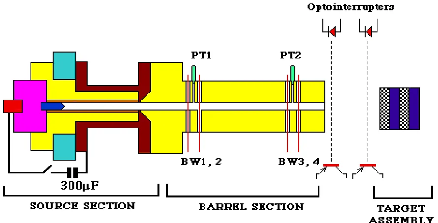
over 50-150 µs. Generally, useful heat flux originates in and is transported from the ET source section, then exposed to test material samples as a near-blackbody radiation source. Aerosol formation from wall material mobilization, however, requires a somewhat different configuration. Heat flux for wall erosion is in effect produced by the same mechanism for the nominal case, but the material of interest is placed within the ET source section and comprises the wall exposed to plasma. Once the eroded material exits the source section, it undergoes expansion and generates aerosol in a large chamber. This process and the necessary changes in SIREN’s configuration are described following a brief overview of normal ET gun operation. The next section details the techniques for characterizing particulate collected during the series of experiments for this investigation. The final section gives the results from a series of scoping tests performed to validate the use of SIRENS for particle production.
3.1. Overview of ET Gun Operation
SIRENS was designed to utilize an electrothermal ablation-controlled arc to generate a high heat flux source for studying plasma-material interaction. The term electrothermal results from the arc discharge vaporizing and heating inner wall material, creating a hot, conductive gas (i.e. plasma). Figure 3.1 shows the configuration of the ET source section.
Electric Power Supply Switch
Electrothermal Plasma Jet Anode
Ablator Cathode
Figure 3.1. Electrothermal source configuration of SIRENS for nominal operation.
characteristics of the vapor of the wall and cathode material rather than that of the fill gas. This brute-force arc generation occurs in an estimated time on order of hundreds of nanoseconds, as determined by the total circuit impedance.
The mechanism by which energy is transferred to the capillary wall is radiation. Since the arc plasma is in LTE (which means no net energy flows between volume elements, electron and arc gas temperatures are equivalent, and the plasma is optically thick), the plasma surface will radiate as a black body. Heat flux to the surface is governed by the Stefan-Boltzmann radiation law, q” = σT4, where σ is Stefan’s constant (5.7605E10-8 W/m2
/K4
) and T is the vapor temperature in K. Ensuing wall vaporization from this incident heat flux results in energy removal by gas-dynamic jets. As the capillary within the ET source provides a constrictive geometry, the gas is ejected into the arc region, partially ionized, and heated to thermodynamic equilibrium. This plasma continues to radiate, and pressure will increase due to mass addition. Since the capillary is open on one end, an axial pressure gradient is formed which forces the plasma to jet out. This dynamic process assumes the relaxation time of thermodynamic equilibrium is much less than any characteristic time associated with gas-dynamic transport.
3.2. SIRENS Specifications
Figure 3.2. Layout of SIRENS, including various diagnostic tools for standard operation.
Table 3.1. SIRENS Operational Characteristics.
Discharge Voltage 1 - 8 kV
Peak Current 20 -100 kA
Net Energy 1 -80 kJ
Discharge Period 100 -300 µs Radiated Power 2 - 120 GW/m2
Peak Pressure 100 - 700 MPa
Plasma Density 1024
- 1027
m-3
Average Temperature 1 - 3 eV Average Velocity 4 - 8 km/s
Table 3.2. Available Diagnostics on SIRENS. Temperature conductivity probes,
Langmuir probes,OMA Pressure piezo-electric pressure
transducers Heat Flux IR thermocouples
Velocity break wires, opto-interuptors Plasma
Composition
OMA
Discharge Voltage
Tektronix high voltage probe
Discharge Current
Rogowski coil
Mass Loss micro-balance scales
plasma in the circuit generates a time dependence in the R and L components, acting to destabilize the governing equation and create a set of coupled equations (generally assumed to be linear). Detailed analysis of this circuit is important to ensure the system is near critically damped, otherwise a large voltage oscillation would send current back into the capacitor bank. The circuit designed for SIRENS has been tested and used for many experiments. Varying pulse lengths, or time constants, are achieved by changing the amount of controllable inductance in the circuit. The present configuration is designed for pulse lengths between 50 µs and 250 µs. Bank charging is accomplished using an external circuit with a 100 mA high- voltage power supply. Once the desired charging voltage is achieved, the charging circuit is isolated and an independent high-voltage thyratron is used to trigger the spark gap switch.
3.3. Modifications for Particulate Study
The versatility of SIRENS proves to be useful in the study of wall material erosion relevant to fusion devices. The experiment has been used to simulate plasma disruption-induced activation product generation and transport in a tokamak, with the detailed objectives described in [21]. Experiments were performed to determine size and chemical form of material mobilized during a plasma disruption. The data will contribute to determination of the overall activation product source term associated with postulated ITER accidents.
Disruption heat flux in ITER is expected to be 20 - 100 GW/m2
(20 - 100 MJ/m2
over 1 - 10 ms), and SIRENS can generate heat flux in the range of 50 GW/m2
(up to 12 MJ/m2
over 0.25 ms). The primary mechanism of energy transfer to the walls in both ITER and SIRENS is radiation heat transport. Thus wall material erosion occurs similarly in both devices. Vapor shielding is not a dominant factor in this comparison because the overall energy deposited to the wall surface is of interest, not the heat flux originating from the source alone. The temperature of the vapor shield (or plasma-surface interaction region) is, however, important because this is a source of radiation. In ITER, continual ablation of surfaces exposed to disruption plasma will feed mass into the interaction region, which is subsequently heated by the incoming flux of energetic particles from the core plasma. In principle, this is analogous to the ablation-controlled arc in the ET source of SIRENS.
Of particular interest in this investigation is what happens to eroded material following the disruption simulation. A significant amount of mass may be mobilized by the disruption. After the disruption ceases, a portion of the vapor component that is not intercepted by a cold wall (resulting in surface condensation) continues to expand into the large volume of the plasma chamber, cooling and condensing as it does so. Similarly in SIRENS, the vaporized wall material is ejected from the capillary into an expansion volume. Cooling and condensing in the expansion volume makes the particles generated in SIRENS to be representative of those expected from an ITER disruption.
Table 3.3 displays a comparison between relevant ITER and SIRENS parameters [22]. Major points displayed by the table are:
• disruption (or simulation) energies and pulse lengths are different
• affected areas are vastly different (SIRENS can accommodate only small samples)
• total power fluxes exposed to wall material are similar (within scale)
• ITER-relevant materials may be studied in SIRENS
• mixed materials effects may be studied experimentally
• adiabatic expansion volume ratios are scalable for a range of vaporized mass
ITER-Table 3.3. Comparison of relevant ITER and SIRENS parameters [22].
Parameter
ITER
(expected) SIRENS
Scaling ITER : SIRENS
1. Disruption energy (MJ/m2) 20 - 100 up to 12 1 : 2 - 1 : 10
2. Energy pulse duration (msec) 1 – 10* up to 0.25** 1 : 4 - 1 : 100 3. Disruption power flux to walls
(GW/m2)
20 – 100 50 1 : 0.4 - 1 : 2
4. Affected area (m2) 10 - 500 7.5E-4***
-5. Expansion volume ratio
Erosion Depth
1 µm 7.69E-8 1.17E-7 1 : 1.5
10 µm 7.69E-7 1.17E-6 1 : 1.5
100 µm 7.69E-6 1.19E-5 1 : 1.5
6. Materials capability
Material
Important
in ITER? SIRENS capable
Copper Yes Yes
Tungsten Yes Yes
SS316 Yes Yes
Carbon Yes Yes
7. Mixed materials capability Yes Yes
* ITER value from thermal quench time as given by ITER GDRD, March, 1996. ** longer pulse lengths can be achieved via PFN modification
*** after source section modification to SIRENS
relevant materials may be studied in SIRENS, and mixed materials studies are easily performed. Beryllium could be tested but is beyond the scope of this investigation due to special handling requirements. Although the simulated disruption energy and pulse length are different from those expected in ITER, the total power flux (GW/m2) achievable in SIRENS is comparable. Similarity in power flux is essential because pseudo-steady ablation rates of radiatively heated surfaces are directly dependent upon this parameter.
may be installed in the pressure tap, although difficulty is encountered in obtaining a meaningful signal due to the electromagnetic interference from the adjacent plasma arc. Another significant change was the addition of a glass expansion chamber with one end connected to the ET source (Figure 3.5). This chamber is necessary to allow controlled collection of the particles produced during the disruption simulation. Chamber expansion volume is limited by the size constraints of the SIRENS vacuum vessel. Chamber dimensions are 180 mm in diameter and 760 mm in maximum length (aspect ratio = L/D = 4.2). The chamber aspect ratio is adjustable by shifting the end-plate position to allow scaling for any reasonable expansion volume. Particulate collection is accomplished by the placement of collection substrates, or ‘buttons’, at various locations on the expansion chamber wall. Particles intercepting buttons adhere to the button surfaces, which are later observed by optical and SEM microscopic techniques to determine particle parameters. Figure 3.6 graphically demonstrates the relative location of collection buttons used in the general test series of this investigation, and Table 3.4 indicates button location coordinates. Some comments regarding the description of button location are in order: (1) end plate is 73.66 cm from source exit, (2) chamber top is aligned to 0˚, and (3) end plate 90˚ is aligned to chamber 0˚. Also, metallic (copper and stainless steel) and glass (quartz) buttons were used to collect particles. Details of the expansion chamber design, button location, and characterization of collected particulate are given in the following section.
3.4. Characterization of the Particulate
This section describes how particulate is collected from experiments in SIRENS and the subsequent construction of particle size distributions from the collected material.
3.4.1 Condensate Collection by Capture Buttons
As described in Section 3.3, vaporized material from SIREN’s ET source expands out into a glass collection chamber. Upon expansion, energy is lost via thermal radiation (the vapor is still very hot when exiting the capillary) since the background gas at low pressure does not significantly contribute to convective cooling. When the vapor reaches the wall, conduction will also assist in cooling. During this expansion and cooling process, condensation will occur by one or more mechanisms. For example, homogeneous and/or heterogeneous nucleation may occur in the bulk expansion plume, while wall condensation (drop-wise or film) could occur at the peripheral boundary.
Vacuum Boundary
Pressure Tap
Anode (SS304)
Outer Insulator (Lexan)
Inner Insulator (Lexan) Isolation Sleeve (MAYCOR) Sample Sleeve
Cathode (HD 17.6- Diemitech) Current Collector Fitting
(Copper)
Figure 3.4. Modified SIRENS source section.
Table 3.4. Tabulated button distribution for the experimental configuration.
Wall Buttons
Button
Axial distance
from source (cm) θ (deg.)
1 12.7 0
2 12.7 180
3 31.75 45
4 31.75 225
5 50.8 90
6 50.8 270
7 69.9 135
8 69.9 315
(Chamber Dimensions: R = 90 mm, L = 760 mm)
End-Plate Buttons
Button Radius (cm) Angle (deg.)
9 3.0 0
10 4.5 45
11 7.0 90
12 7.0 180
13 3.0 225
14 4.5 270
15 7.0 315
16 4.5 135
17 4.5 224
0 10 20 30 40 50 60 70 80 cm
1,2
3 4
5 6
7 8 Source
End Plate
θ˚
End Plate Distribution: Expansion Cell Distribution:
9 10 11
12
13
14 17
15
16
X
plexiglass
end plate buttons
90˚
0˚ 135˚
180˚
225˚
270˚
315˚ 45˚
Pressure tap
diameter = 17.8 cm
expansion. Thermal radiation cooling, however, does occur and drives the vapor into thermal non-equilibrium condensation at a faster rate than adiabatic expansion alone. An added complication is gas-dynamic non-equilibrium which results from free-jet expansion of the vapor from the source exit into the chamber. Occurrence of these non-equilibrium processes shows that vapor expansion from the source section is not truly adiabatic. The volume required for adiabatic expansion will be used as a reference against which to compare the experimental expansion volume. For example, an initial pressure of 500 MPa will be obtained for 1 gram of Cu vaporized at 0.5 eV in the volume of the source section (this estimate is from expected experiment conditions), and a final expansion pressure of 101.325 kPa (Cu is solid at 1 atmosphere) to yield a high level of supersaturation, the required volume for adiabatic expansion of the ideal gas is 2.5 x 10⁻⁴
m3
. Applying the ideal gas equation of state gives a final vapor temperature of 192 K, for which the saturation pressure is ~ 10 Pa; hence the vapor is supersaturated and will certainly condense. Volume available to the real gas is 3.14 x 10⁻³
m3
with the dimensions (100 mm diameter and 400 mm length) of the chamber used in the scoping studies of Section 3.5, providing 12.6 times the adiabatic expansion volume. A larger chamber (180 mm diameter and 762 mm length) is used in the experiment test series, providing an expansion volume of 1.94 x 10⁻²
m3
, or 77.6 times the adiabatic expansion volume for the given example. This chamber is of the largest size that could be placed in the SIRENS vacuum vessel, and should be sufficient to allow expansion cooling of most of the vapor quantities expected in the test series.
Once particles have formed within the chamber, they either follow flow streamlines or diffuse to the wall. To collect these particles, 1.25 cm diameter discs (buttons) are distributed on the inner wall. As a preliminary test, stainless steel (SS316) was used for Cu source section samples and copper was used for SS316 samples. General button distribution was shown in Figure 3.6 of the previous section. Vapor and particle momentum near the ET source exit are predominately directed along the chamber axis, resulting in fewer particles transported to the wall and increased mass deposition down the length of the chamber. Buttons approaching the end of the chamber are placed at offset locations that will eliminate deposition shadowing by upstream buttons. At the very end of the chamber, buttons are placed on a plastic end plate. Maximum mass deposition is expected at this location.
Buttons are attached by adhering the discs to plastic backings (using rubber cement, which allows them to be easily removed with acetone). The backings are tapped to accept threaded rods that penetrate tiny holes in the chamber wall and are capped with small nuts. This arrangement allows for button installation prior to an experiment and removal following an experiment.
in a control set of 4 buttons was individually weighed, attached to the plastic backing, threaded with the rod, and attached to the chamber wall. An equivalent procedure is used in preparation for an experiment test. Next, the button sets were removed from the chamber, taken off the plastic backing, and re-weighed. Table 3.5 displays the initial and final weights measured during this test. The difference is within the uncertainty of the measurement (+ 0.00003 g), thereby showing that mass deposition on buttons can be determined from weight measurements before and after exposure.
Once a shot is complete and particles have been deposited on the buttons, they are removed from the expansion chamber, weighed, and prepared for particulate size distribution analysis. Characterization of particle size and morphology using a scanning electron microscope (SEM) and an optical microscope are discussed in detail in the following sections.
Table 3.5. Control button analysis.
Control Button
Initial Disc Weight* (grams)
Final Disc Weight*
(grams) % difference
1 0.58233 0.58231 0.003
2 0.58380 0.58382 0.003
3 0.58262 0.58260 0.003
4 0.58356 0.58354 0.003
*- average of 4 different measurements.
3.4.2 Observation of Particulate
Scanning electron microscopy (SEM) and optical microscopy techniques have been developed for characterizing particulate from various sources [23]. Size distributions are readily generated by counting the number of particles within a specified size range on images obtained at various magnifications. Analysis of the particles produced during a disruption simulation on SIRENS will be accomplished in this manner. The capture buttons will serve as both collection surfaces and as analysis substrates.
magnifications could result in over-counting the number of particles in size bins that are shared between the distributions from each magnification. The overall particle size distribution construction protocol is described in Section 3.4.3. The number of photographs necessary at a specified magnification is influenced by the observed particle density on the image. Many particles must be counted for sufficient counting statistics to ensure accurate representation of the size distribution. Generally, four areas should be examined and photographed at each magnification. For the scoping tests reported in Section 3.5, only one photograph was available in many cases.
Figure 3.7 displays resulting SEM photographs of a particular button (S715 Button 11) used to collect particles in one of the scoping experiments. Part (a) of Figure 4.2.1 shows an SEM image at 500x, where many particles are present. Based on experience gained from using this method, this magnification would be used to count particles greater than 2.5 µm. Part (b) of the figure was taken at 1200x, which, for example, could be used to count particles between 0.625 µm and 2.5 µm. An image with magnification 3000x is shown in part (c). This magnification would be used to count particles in the size range of 0.1 µm to 0.625 µm. In this example, several images at 3000x would be required for analysis because there are relatively few particles present to contribute to the overall distribution. Generally, images obtained at magnifications higher than 3000x on the SEM are impractical because many photographs would be necessary to obtain a representative count of particles less than 0.1 µm. With both the SEM and optical microscope, the minimum counted particle size is dependent upon the highest magnification and the number of photographs taken at that magnification. If a sufficient population of extremely small particles (< about 0.25 µm) are observed, many photographs are made to accurately represent them in the overall distribution.
Figure 3.8 shows the resulting 100x, 500x, and 1000x optical microscope photographs for S715 Button 10. The optical microscope can be used similar to the SEM microscope following the same guidelines for image quality and quantity.
(a) Magnification of 500x (b) Magnification of 1200x
(c) Magnification of 3000x Figure 3.7. SEM micrographs from button 11 of scoping test S715.
(a) 100x photo (b) 500x photo
(c) 1000x photo Figure 3.8. Continued.
3.4.3 Image Analysis and Generation of Size Distributions
Image analysis and particle counting for this investigation is accomplished by extending the method developed in [10], with specific enhancements made by the author. A schematic depiction of the technique is shown in Figure 3.9. As described in Section 3.4.2, the substrates are examined using a scanning electron microscope and an optical microscope. The images are analyzed using NIH-Image, available as public domain software from the National Institute of Health. Photograph images are scanned and converted to digital files that are used as input to the software. The digital image is prepared for object counting (i.e. scaling, thresholding, shadow removal, etc.) and the software is instructed to “analyze particles.” Results for each particle on the image are returned and include projected area (from pixel-area scaling conversion), major and minor elliptical radii, and any user defined function, such as conversion of projected area to equivalent-sphere diameter. The resulting data from each individual photograph of a given substrate are combined and used to build the particle size distribution using a spreadsheet.
The first step following image acquisition and particle count involves performing a sampling test known as the Kruskal-Wallis test on data sets taken at the same magnification but at different locations on the substrate. This test determines if the data sets are representative of the overall underlying population. Data sets that fail this test are eliminated from the analysis. The next step is to define size bins for each magnification and count the number of particles that contribute to each bin range at each magnification. From this, cumulative percent of counted particles is determined for each magnification. These magnification distributions are then plotted in log-probability form and a linear fit applied. The count median diameter (CMD) and geometric standard deviation (GSD) are determined from the fit parameters. The CMD, d50%, is the particle size corresponding to the 50%
cumulative value and the d84.1% is the particle size corresponding to the 84.1% cumulative
value. For a log-normal distribution, the GSD is the d84.1% value divided by the d50% value.
Aquire Photographs
NIH-Image Analysis
Bin and Size in Excel
Kruskal-Wallis Statistical Test
Determine Cumulative Distribution for each
Magnification
Determine Size Ranges for Each
Magnification
Apply Area Based Scaling Factors
Combine Data from each Magnification and Build Overall Distribution
Calculate 95% Confidence
Intervals
Plot Cumulative Distribution
Calculate
d50%, d84%, R, and GSD
Figure 3.9. Schematic depiction of the size distribution construction technique.
magnification is made. Data in the appropriate size range for each magnification are then scaled by adjusting the number of counts in each bin based on the viewed area of that magnification. Table 3.6 shows the scaling factors used for various magnifications for both SEM analysis and optical microscope analysis. Scale factors for the optical microscope were obtained by photographing a reference slide with etch marks spaced at known (small) distances, then measuring pixel distance in the corresponding electronic image. Scale factors for the SEM are calibrated in a similar fashion. Once obtained, the scaled counts are combined to produce the overall particle size distribution for the substrate under investigation. Distribution CMD and GSD are obtained from linear fit parameters, and the linear correlation coefficient (R2) is reported. Ninety-five percent confidence intervals for the distribution are also calculated and plotted.
To verify the distribution construction technique, a particle size distribution was constructed from optical microscope photographs provided by the INEEL of sample Q1DV taken from the DIII-D tokamak vacuum vessel. Table 3.7 shows a summary of the relevant particle size distribution data generated for the comparison as well as the data reported in [10] for the sample analyzed. Figure 3.10 shows the distribution constructed by NCSU from the DIII-D Q1DV photographs provided by the INEEL and the distribution generated from INEEL’s separate analysis of the same data. Differences in the values obtained for d50%
The particle size distribution measurement has been benchmarked as outlined in [10]. using known particle size distribution material obtained from Duke Scientific, CA, USA.
Table 3.6. Scale Factors for the optical microscope and the SEM microscope. Magnification Optical Microscope Scaling SEM Microscope Scaling
(pixels/µm)(a) Scale Factor (pixels/µm)(a) Scale Factor
50x 0.342 0.25 -
-100x 0.679 1 -
-350x - - 1.97 0.49
500x 3.4 25 2.95 1
700x - - 2.74 1.96
1000x 6.8 100 5.9 4
1200x - - 7.2 5.76
1500x - - 8.9 9
3000x - - 17.7 36
5000x - - 19.5 100
(a) Magnifications are constant as determined by the microscope hardware. Scale values may vary slightly if digitized at higher magnification than one. This is accounted for by the operator using NIH-Image by measuring the area of each photograph.
Table 3.7. Comparison of NCSU analysis verses INEEL analysis for DIII-D Q1DV.
d15.9% (µm) d50% (µm) d84.1% (µm) GSD R
2
NCSU Analysis 0.25 0.64 1.65 2.59 0.9857
0 1 10 100
.001 .01 .1 1 5 10 20 30 50 70 80 90 95 99 99.9 99.99 99.999
Log-Probability Plot for DIII-D Dust (NCSU Analysis)
Particle Diameter (µm)
Percent less than indicated size distribution parameters 0.25 µm d 15.9% 0.64 µm d 50% 1.65 µm d 84.1% 0.98569 R2 2.59 GSD analysis summary counted size range (µm) total number of particles area (µm2)
magnification, number of photos
d
p > 6.5 µm
4,563 8,818,618
50x, 4
3 < d
p < 6.5
1,859 1,102,053
100x, 2
1.75 < d
p < 3
6,553 687,976
200x, 4
0.75 < d
p < 1.75
2,521 88,370
500x, 4
0 < d
p < 0.75
1,413 22,065 1000x, 4 0.1 1 10 100
.001 .01 .1 1 5 10 20 30 50 70 80 90 95 99 99.9 99.99
99.999
Log-Probability Plot 0f DIII-D Q1DV Dust (INEEL Analysis)
Particle Diameter (µm)
Percent less than indicated size distribution parameters 0.18 µm d 15.9% 0.53 µm d 50% 1.52 µm d84.1% 0.98234 R2 2.88 GSD Detail Vacuum Range Magnification
0 - 1.0 µm 1000x
1.0 - 1.5 µm 500x
Not Used 200x
1.5 - 4.5 µm 100x
4.5 µm and up 50x
3.5. Scoping Test Results
The new experimental configuration and the particle size analysis technique just described were implemented in scoping tests prior to initiating a full test series. Four experimental runs, or “shots”, were completed, with three producing particle size distribution results. Table 3.8 displays a summary of the scoping shots. Data-recording trigger failures hindered shot duration measurements (obtained from discharge current measurements) for S712 and S715. This problem has been corrected. Shot duration measured for S713 was 40 µs, producing an energy flux of 115 GW/m2
incident on the sample material (Cu).
Table 3.8. Scoping Shots Summary.
Sleeve Dimensions Shot
Label
Energy (kJ)
Duration
(µsec) Sample ID length
Sample ∆m
(mg) comments
S710 2.5 10 Cu - 12 mm 100 exploding wire
S712 4.9 - Cu 4 mm 6 mm 490 diagnostics trigger failed
S713 5.2 40 Cu 4 mm 6 mm 320 filter installed
S715 3 - SS316 4 mm 6 mm 197 diagnostics trigger failed
3.5.1 Shot S710
The first test performed, S710, involved introducing a copper wire into the capillary of the ET source section. When sufficiently high current (10-20 kA) is passed through this wire, it is heated very rapidly and vaporizes. This mechanism generates an inventory of metal vapor within the capillary that is ejected due to the resulting pressure gradient. Such a process is somewhat similar to what occurs during generation of an electrothermal plasma. It is not, however, suitable as a method for disruption simulation because the mechanism of material heating is different from that in a disruption (i.e. Joule heating vs. radiative heat flux). This technique is, however, suitable to evaluate the expansion chamber for particulate collection.
the surface in a consistent manner. Resulting particle size distributions could not be generated because of the insufficient number of particles collected from the wall. An alternative method of collecting and analyzing the particles was developed using collection buttons attached to the wall of the expansion chamber, as described in Section 3.4. An acid bath was used to remove all the copper particles from the wall in this shot.
3.5.2 Shots S712 and S713
The first material to be tested in the modified ET source section was copper. Shots S712 and S713 were an attempt to generate, collect, and analyze copper particulate from a disruption simulation.
S712 was performed with buttons distributed along the collection chamber wall and also on a plastic plate attached to the end of the expansion chamber. The shot was performed at an energy level of 4.9 kJ (measured from capacitor bank loss), and resulted in 490 mg of mass removed from the copper sleeve in the source section. Unfortunately the manual diagnostics trigger on the delay generator failed to trigger the current and voltage recordings, so integrated power was not obtained. This problem can be attributed to the problems associated with the electronic data acquisition modules used to record the current and voltage. The problem has been corrected by repairing and recalibrating the data acquisition modules (LeCroy 6810). These shots were successful in that copper particulate was produced in the experiment and collected on the button substrates. In contrast to the exploding wire test, these particles were somewhat loosely attached to button surfaces and the chamber wall. A simple swipe with a Q-tip would displace and remove the dust from the wall. Deposition along the wall (viewed as a slight copper-colored haze) was not uniform but tended to be thicker at the chamber’s end. Dust appeared to pile in front of the buttons on the chamber wall. Deposition on the buttons varied, however there was a shadowing effect from other buttons upstream. To avoid this in future shots, axially consecutive buttons were rotated azimuthally in the chamber. Also in this shot, the end section of the glass collection chamber broke into several pieces, indicating the existence of a significant pressure wave at that location some time during the expansion. This broken end was removed and the plastic end plate was inserted, which survived all subsequent shots.
S713 Current Trace
-40 -20 0 20 40 60 80
0E+0 2E-5 4E-5 6E-5 8E-5 time, sec.
Current, kA
S713 Voltage Trace
-1 0 1 2 3 4 5 6
0E+0 2E-5 4E-5 6E-5 8E-5
time, sec.
Voltage, kV
Figure 3.11. S713 current and voltage traces.
of dust similar to that of S712 was observed in the chamber following shot execution. Unfortunately the filter substrate (cellulose nitride) burned away, indicating exposure to hot vapor. As expected, particulate deposition occurred on collection buttons distributed along the wall and end section around the filter housing.
much less than the mass loss measured from the source section (320 mg). Accounting for collection of all mass evolved from the source section is impractical because of the difficulty of accounting for mass deposited in a non-uniform fashion along the length of the expansion chamber.
Table 3.9. Summary of Particle Size Distribution Data for S712 and S713. S712 Button
Axial distance
from source (cm) d15.9% d50% d84.1% GSD R
2
14 40.6 0.57 1.15 2.31 2.01 0.9642
19 42.5 (end plate) 0.46 0.95 1.94 2.04 0.9868
20 42.5 (end plate) 0.22 0.47 1.01 2.15 0.9845
S713 Button
Axial distance
from source (cm) d15.9% d50% d84.1% GSD R
2
1 4.5 0.24 0.55 1.24 2.25 0.9858
11 40 (end plate) 0.15 0.51 1.67 3.27 0.9436
(a) S712 Button 14 (b) S713 Button 11
Figure 3.12. SEM micrographs from S712 and S713.
0.1 1 10
.01 .1 1 5 10 20 30 50 70 80 90 95 99 99.9
99.99
S712 Button 14 Overall Distribution
Particle diameter (µm)
Percent less than indicated size distribution parameters
0.57 µm d
15.9%
1.15 µm d
50%
2.31 µm d
84.1%
2.01 GSD
0.96419 R2
analysis summary
counted size range (µm) total number
of particles area (µm2
) magnification,
number of photos
d p > 1.25 171
75,170 350x, 1
0 < d p < 1.25 50
6,434 1200x, 1
not used 30
1,035 3000x, 1
0.1 1 10
.01 .1 1 5 10 20 30 50 70 80 90 95 99 99.9
99.99
S712 Button 19 Overall Distribution
Particle diameter (µm)
Percent less than indicated size distribution parameters 0.46 µm d 15.9% 0.95 µm d 50% 1.94 µm d 84.1% 2.04 GSD 0.98683 R2 analysis summary counted size range (µm) total number of particles area (µm2
) magnification,
number of photos
d p > 0.8 925
19,516 700x, 1
0 < d p < 0.8 551 6,584 1200x, 1 not used 72 382.4 5000x, 1 0.1 1 10
.01 .1 1 5 10 20 30 50 70 80 90 95 99 99.9
99.99
S712 Button 20 Overall Distribution
Particle Diameter (µm)
Percent less than indicated size distribution parameters 0.22 µm d 15.9% 0.47 µm d 50% 1.01 µm d 84.1% 2.15 GSD 0.98446 R2 analysis summary counted size range (µm) total number of particles area (µm2
) magnification,
number of photos
d p > 1.0 1045
93,034 350x, 1
0 < d p < 1.0 349
373.3 5000x, 1
0.1 1 10
.01 .1 1 5 10 20 30 50 70 80 90 95 99 99.9
99.99
S713 Button 1 Overall Distribution
Particle diameter (µm)
Percent less than indicated size distribution parameters 0.24 µm d 15.9% 0.55 µm d 50% 1.24 µm d 84.1% 2.25 GSD 0.9858 R2 analysis summary counted size range (µm) total number of particles area (µm2
) magnification,
number of photos
d
p > 1.1
518 78,392
350x, 1
0 < d
p < 1.1
382 6,417 1200x, 1 0.1 1 10 100
.01 .1 1 5 10 20 30 50 70 80 90 95 99 99.9
99.99
S713 Button 11 Overall Distribution
Particle diameter (µm)
Percent less than indicated size distribution parameters 0.15 µm d 15.9% 0.51 µm d 50% 1.67 µm d 84.1% 3.27 GSD 0.94357 R2 analysis summary counted size range (µm) total number of particles area (µm2)
magnification, number of photos
d p > 2.0 157
79,289 350x, 1
0 < d p < 2.0 218
4,560 1200x, 1