Pole-Zero Analysis of Microwave Filters Using Contour Integration
Method Exploiting Right-Half Plane
Eng Leong Tan and Ding Yu Heh*
Abstract—This paper presents the pole-zero analysis of microwave filters using contour integration method exploiting right-half plane (RHP). The poles and zeros can be determined with only S21 by exploiting contour integration method on the RHP along with certainSmatrix properties. The contour integration in the argument principle is evaluated numerically via the finite-difference method. To locate the poles or zeros, the contour divide and conquer approach is utilized, whereby the contour is divided into smaller sections in stages until the contour enclosing the pole or zero is sufficiently small. The procedures to determine the poles and zeros separately are described in detail with the aid of pseudocodes. To demonstrate the effectiveness of the proposed method, it is applied to determine and analyze the poles and zeros of various microwave filters.
1. INTRODUCTION
Microwave filters [1–9] have been designed, synthesized and analyzed over the years for various applications. Most analyses in the literature have not considered the poles and zeros of the synthesized filters on the complex frequency (s) plane. These poles and zeros are often not ascertained thoroughly after design stages and their locations are commonly deduced vaguely from the plots of S parameters, which may depict some reflection zeros, etc. Note that the plots ofS parameters versus real frequencies only provide the frequency responses along thejω axis and do not provide sufficient information on the complexsplane. Furthermore, it is rather difficult to solve for the poles and zeros of filters designed using transmission line structures, especially when the lines are non-commensurate. This is because the overall S parameter expressions contain non-polynomial transcendental functions and conventional methods such as Richard or Euler transformations are inadequate. For filters designed using lumped elements such as inductors and capacitors, the polynomial coefficients could also be rather ill-conditioned [10]. To alleviate the difficulty and inadequacy, we have proposed the use of contour integration method based on argument principle to determine the poles and zeros of microwave filters [11]. To include lossless filters with complex zeros, the Belevitch theorem is applied to separate the poles and zeros in different half-plane regions. Such separation of poles and zeros involve evaluation ofSmatrix (Belevitch) determinant [12]. Using the Belevitch determinant and contour integration method, the poles and zeros of lossless filter transfer functions can be determined separately with certainty. Note that in [11], the contour integration method is evaluated on the left-half plane (LHP) only, as one would generally do since all poles are located on the LHP for stable system.
In this paper, we present an alternative approach for pole-zero analysis using contour integration method exploiting right-half plane (RHP). The poles and zeros can be determined with only S21 by exploiting contour integration method on the RHP along with certain S matrix properties. Hence, there is no need to evaluate theS matrix determinant that involves all its entriesS11,S12,S21andS22. In Section 2, the argument principle and contour integration method will be discussed. The contour
Received 23 October 2018, Accepted 16 January 2019, Scheduled 22 January 2019 * Corresponding author: Ding Yu Heh ([email protected]).
integration in the argument principle is evaluated numerically via the finite-difference method. To locate the poles or zeros, the contour divide and conquer approach will be utilized, whereby the contour is divided into smaller sections in stages until the contour enclosing the pole or zero is sufficiently small. The procedures to determine the poles and zeros separately will be described in detail with the aid of pseudocodes. In Section 3, the proposed method will be applied to determine and analyze the poles and zeros of various microwave filters.
2. EXPLOITING CONTOUR INTEGRATION METHOD ON THE RIGHT-HALF PLANE TO DETERMINE POLES AND ZEROS SEPARATELY
2.1. Argument Principle and Contour Integration Method
The argument principle is expressed as [13]
C f(z)
f(z)dz= 2πj(Z−P). (1)
where Z and P are the total numbers of zeros and poles for a meromorphic function f(z) within the closed contour C, including their multiplicities. The contour C is taken in counter-clockwise oriented path, andf(z) is the derivative of the complex function. Applying the argument principle, the complex functionf(z) is replaced byS21(s) of a microwave filter on the complexsplane, wheres=σ+jω. The contour integration off =S21 can be evaluated numerically via
C S21 (s) S21(s)ds =
s
S21(s+ Δs/2)−S21(s−Δs/2) Δs
S21(s) ·Δs
=
s
S21(s+ Δs/2)−S21(s−Δs/2)
S21(s) , (2)
where central finite-differencing is used for the derivative S21 (s), and Δsis the spatial step size chosen along the path to ensure convergence. To evaluate the numerical contour integration in Eq. (2), the overall analyticalS21expression is not required, while only the numerical values ofS21along the contour path are needed. In practice, for microwave filter circuits, the circuit parameters for individual sections (such as transmission lines, lumped elements, etc.) can be computed and manipulated readily to obtain theS21values of the overall circuits. Note that all the circuit sections are taken to be lossless following the common practice in the conventional synthesis of microwave filters.
The number of poles for a microwave filter within the contour can be determined from contour integration method in Eq. (2) if the number of zeros,Z, is known, orvice versa, based on the following:
P = −1 2πj
s
S21(s+ Δs/2)−S21(s−Δs/2) S21(s)
+Z, with Z known, (3a)
Z = 1
2πj
s
S21(s+ Δs/2)−S21(s−Δs/2) S21(s)
+P, withP known. (3b)
arranged about the imaginary axis on the complex s plane [5]. Hence, if complex zeros exist on the LHP, they can also be found on the RHP symmetrically located about the jω axis. By evaluating Eq. (3b) on the RHP and setting P = 0 since there is no pole on RHP for stable system, we are able to determine the number of zeros on the RHP and LHP due to symmetrically located zeros. With Z determined, it can now be substituted into Eq. (3a) to determine the number of poles on the LHP. As such, the poles and zeros can be determined separately with certainty. From (3), we see that only S21 of the filter is needed. There is no need to evaluate the S matrix determinant in [11] that involves all its matrix entriesS11,S12, S21and S22.
2.2. Contour Divide and Conquer Approach
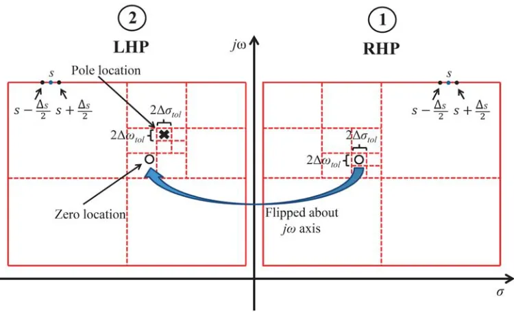
In the previous subsection, the contour integration method determines the total number of poles and zeros within the enclosed contour. After finding the total number of poles and zeros, we proceed to locate them along with their respective order via the contour divide and conquer approach. In this approach, the contour is to be divided into smaller sections in stages until the contour enclosing the pole or zero is sufficiently small. In this case, the location of the pole or zero is bounded within a sufficiently small enclosed contour, and the number of pole or zero represents their respective order. The procedures of contour divide and conquer approach are better illustrated in Fig. 1. As shown in the figure, we divide the contour area into four smaller sections (dashed) in each stage successively before enclosing a pole or zero with specified tolerances. The contour is first applied on the RHP to find the zeros. They are then flipped about the imaginary (jω) axis to obtain the LHP zeros. Once the complex zeros are located, the poles can be found readily. In particular, the contour is applied onto the LHP to find the poles, with known zeros found earlier. Although only one pole or zero is shown here, the approach in general will arrive at all poles and zeros enclosed within the contour. The procedures are described in detail with the aid of pseudocodes below. The contour on the RHP is described in Pseudocode 1, followed by contour on the LHP described in Pseudocode 2.
Figure 1. Illustration of contour divide and conquer approach, first applied on the RHP and then on the LHP.
Pseudocode 1 — on the RHP:
1. Given a set of contour rectangles Rri on the RHP.
the given {Rir} on the RHP. 3. Initialize Rrnew={ };
4. For each saved{Rri}, {
4.1 If the {Rri} bounds Δωi and Δσi exceed tolerance {
4.1.1 Divide Rri into smaller{Rrsj} 4.1.2 For each {Rrsj}
{
4.1.2.1 Compute Eq. (3b) forZsj withPsj = 0.
4.1.2.2 If Zsj >0,{Rrnew} ← {Rrnew} ∪ {Rrsj}, save Zsj. }
} 4.2 Else
{
4.2.1 {Rnewr } ← {Rnewr } ∪ {Rri}, save Zi. }
}
5. If{Rri} ={Rrnew}, set {Rri} ={Rrnew}, loop back to Step 3. Else, exit and go to Step 6.
6. Flip {Rir} about jω axis onto LHP, i.e., {Rri} ← {−Rri∗}, where superscript ∗ indicates complex conjugate. We have now retrieved all LHP zeros (knowing all Zi’s). Proceed to Pseudocode 2 to retrieve the poles.
Pseudocode 2 — on the LHP (with known zeros Zi’s from Pseudocode 1): 1. Given a set of contour rectangles {Ri} on the LHP.
2. Compute Eq. (3a) for Pi with known Zi. Save only the rectangles {Ri}that have Pi>0. After this step, each saved {Ri} has at least one pole. If none of{Ri} is saved, then exit with no pole within the given {Ri}on the LHP.
3. Initialize Rnew={ }; 4. For each {Ri},
{
4.1 If the {Ri} bounds Δωi and Δσi exceed tolerance {
4.1.1 Divide Ri into smaller {Rsj} 4.1.2 For each {Rsj}
{
4.1.2.1 Compute Eq. (3a) for Psj with knownZsj. 4.1.2.2 If Psj >0,{Rnew} ← {Rnew} ∪ {Rsj}, save Psj. }
} 4.2 Else
{
4.2.1 {Rnew} ← {Rnew} ∪ {Ri}, save Pi. }
}
5. If{Ri} ={Rnew}, set {Ri}={Rnew}, loop back to Step 3. Else, exit.
yield excessively large value or deviate very much from integer of 2πj. To circumvent this, the contour path at any stage is readjusted±Δω or±Δσuntil Eq. (2) is evaluated to be sufficiently close to integer of 2πj. In doing so, proper convergence of the contour in locating all poles and zeros is ensured. Note that the computational burden of our contour integration method depends only on the (one-dimensional) contour path length for which Eq. (2) is to be evaluated, as compared to the (two-dimensional) area search of complex roots that would be much more expensive in general.
3. APPLICATION EXAMPLES
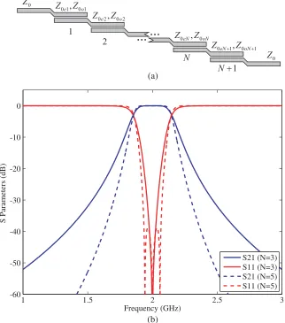
The contour integration method is now applied to solve for poles and zeros of microwave filters. We first look at an example of classical coupled line filter [1]. The layout of coupled line filter comprising N + 1 sections with even and odd characteristic impedances in each individual section is shown in Fig. 2(a). The filter specification is Butterworth response withN = 3, center frequencyf0 = 2 GHz and fractional bandwidth F BW = 0.15. The filter response can be determined by computing the overall ABCD parameters from individual sections which are subsequently converted intoS parameters using standard formula. TheS parameters are plotted in Fig. 2(b), in which one reflection zero is seen in the S11 plot for N = 3. One can see that the number of reflection zeros does not commensurate with the order of the filter. Hence, the filter order cannot be inferred directly from the number of sections or reflection zeros. To analyze the poles, the contour integration method is employed, and the poles of the filter are plotted in Fig. 3. To verify its Butterworth response, a reference Butterworth circle is shown,
0
Z
0
Z
1 0 1e, 0 1o
Z Z
0 2e , 0 2o
Z Z
0eN 1, 0oN1
Z + Z +
0eN, 0oN
Z Z
2
N
1
N+
... ...
1 1.5 2 2.5 3
-60 -50 -40 -30 -20 -10 0
Frequency (GHz)
S Parameters (dB)
S21 (N=3) S11 (N=3) S21 (N=5) S11 (N=5)
(a)
(b)
Figure 3. Poles of Butterworth response coupled line filter withN = 3.
with radiusR scaled to f0 and F BW as
R = f0F BW
2 . (4)
One can see that three poles are distributed along the reference Butterworth circle, which validates its Butterworth response. However, there are also additional two poles located further away from the circle and jω axis. One should take note that although located further away from the jω axis, these additional poles may still contribute to errors in the real and imaginary parts of S21 [11].
We next proceed to analyze the Buttwerworth response coupled line filter with N = 5. The S parameters are shown in Fig. 2(b) and the poles are plotted in Fig. 4. From the figure, one can observe that apart from the additional two poles now moving closer to the circle, the five poles for N = 5 have deviated from the reference circle. Using contour integration method, we demonstrate that the poles of a synthesized filter may deviate from the originally specified ones. This also explains why the S11 plot of the Butterworth response filter in Fig. 2(b) exhibits three reflection zeros, since the poles have deviated from the reference Butterworth circle.
Figure 4. Poles of Butterworth response coupled line filter withN = 5.
Figure 5. Schematic of cross coupled filter.
0.77 0.78 0.79 0.8 0.81 0.82
-100 -90 -80 -70 -60 -50 -40 -30 -20 -10 0
Frequency (GHz)
S Parameters (dB)
S21 S11
0.015 0.01 0.005 0 0.005 0.01 0.015 0.78
0.785 0.79 0.795 0.8 0.805 0.81 0.815
σ/2π
ω
/2
π
(GHz)
(a) (b)
Figure 6. (a) S parameters of cross coupled filter. (b) Poles and zeros of cross coupled filter and reference Chebyshev ellipse.
poles and zeros of the filter are determined and plotted in Fig. 6(b). It can be observed that seven poles are visible within the passband. To verify its Chebyshev response, a reference Chebyshev ellipse is drawn, with major and minor radii, aandb (scaled to f0 and F BW inR) given by [3]
a=R1 +η2, b=Rη (5)
where
η = sinh
1 N sinh
−1 1 E
E = 10LAr10 −1.
We see that the poles are distributed along the reference Chebyshev ellipse, which validates its Chebyshev response. Moreover, there is a pair of symmetrical complex zero at around±0.01 +j0.8 GHz about thejωaxis. This further shows the effectiveness of our proposed method in retrieving both poles and zeros on the complex plane.
So far we have applied the contour integration method to locate the poles and zeros of single band filters, we shall now illustrate its application to dual band (or multiband) filters. We use the example of test filter 1 from [7], whereby two passbands range from 0.96 to 1.6 GHz and 2.02 to 2.68 GHz with seventh-order Chebyshev response and passband ripples LAr = 0.01 dB. The schematic of the dual band filter is shown in Fig. 7, comprising non-commensurate transmission lines with predetermined characteristic impedances and electrical lengths. The S parameters are shown in Fig. 8(a), including the measurement results from [7]. The contour integration method is then applied to determine the
Figure 7. Schematic of dual band filter.
0 0.5 1 1.5 2 2.5 3 3.5 4
-60 -50 -40 -30 -20 -10 0
Frequency (GHz)
S
Parameters (dB)
S21 S11 S21 (Meas.) S11 (Meas.)
1 0.5 0 0.5
1 1.5 2 2.5 3
σ/2π
ω
/2
π
(GHz)
(a) (b)
1 0.5 0 0.5
1 1.5 2 2.5 3
σ/2π
ω
/2
π
(GHz)
Figure 9. Poles for quarter wavelength short-circuited stubs and reference Chebyshev ellipse.
poles within each passband. Fig. 8(b) plots the poles location on the complex s plane. Seven poles are found in each passband, which confirms its seventh-order characteristics. To verify its Chebyshev response, a reference Chebyshev ellipse is also drawn for each band. In this case, it can be seen that although the dual band filter is originally designed according to the given specifications, some poles have deviated from the reference Chebyshev ellipse after realization. To investigate such deviation further, let us examine the poles of quarter-wave short-circuited stubs that constitute the dual band filter. The parameters of the circuited stubs are given in [7, Table I]. Fig. 9 plots the poles for the short-circuited stubs and reference Chebyshev ellipse. It can be seen that the poles have actually deviated from the reference Chebyshev ellipse. Hence, they may explain the deviation of the poles in Fig. 8(b). Thus, the realized poles should be ascertained for further adjustment and tuning if necessary. Through these examples, we have demonstrated the usefulness of the contour integration method in determining the poles and zeros of microwave filters. Finally, it should be noted that the contour integration method herein is applicable not only to microwaves but also to other frequencies such as mmW, sub-THz, etc. [14].
4. CONCLUSION
This paper has presented the pole-zero analysis of microwave filters using contour integration method exploiting RHP. The poles and zeros can be determined with onlyS21by exploiting contour integration method on the RHP along with certain S matrix properties. The contour integration in the argument principle has been evaluated numerically via the finite-difference method. To locate the poles or zeros, the contour divide and conquer approach has been utilized, whereby the contour is divided into smaller sections in stages until the contour enclosing the pole or zero is sufficiently small. The procedures to separately determine the poles and zeros have been described in detail with the aid of pseudocodes. To demonstrate the effectiveness of the proposed method, it has been applied to determine and analyze the poles and zeros of various microwave filters.
REFERENCES
1. Pozar, D. M., Microwave Engineering, 4th edition, Wiley, New York, 2011.
3. Hong, J. S. and M. J. Lancaster, Microstrip Filter for RF/Microwave Application, 2nd edition, Wiley, New York, 2011.
4. Collin, R. E.,Foundations for Microwave Engineering, 2nd edition, IEEE Press, 2001.
5. Cameron, R. J., C. M. Kudsia, and R. R. Mansour,Microwave Filters for Communication Systems, John Wiley and Sons, New Jersey, 2007.
6. Wang, X., Y. Di, P. Gardner, and H. Ghafouri-Shiraz, “Frequency transform synthesis method for cross-coupled resonator bandpass filters,” IEEE Microw. Wireless Compon. Lett., Vol. 15, No. 8, 533–535, Aug. 2005.
7. Liu, A.-S., T.-Y. Huang, and R.-B. Wu, “A dual wideband filter design using frequency mapping and stepped-impedance resonators,” IEEE Trans. Microw. Theory Tech., Vol. 56, No. 12, 2921– 2929, Dec. 2008.
8. Xue, S. J., W. J. Feng, H. T. Zhu, and W. Q. Che, “Microstrip wideband bandpass filter with six transmission zeros using transversal signal-interaction concepts,” Progress In Electromagnetics Research C, Vol. 34, 1–12, 2013.
9. Xu, J. and W. Wu, “Compact microstrip dual-mode dual-band band-pass filters using stubs loaded coupled line,” Progress In Electromagnetics Research C, Vol. 41, 137–150, 2013.
10. Sun, X. and E. L. Tan, “Dual-band filter design with pole-zero distribution in the complex frequency plane,”2016 IEEE MTT-S Int. Microw. Symp. Dig., 2016, doi:10.1109/MWSYM.2016.7540174. 11. Tan, E. L. and D. Y. Heh, “Application of Belevitch theorem for pole-zero analysis of microwave
filters with transmission lines and lumped elements,” IEEE Trans. Microw. Theory Tech., Vol. 66, No. 11, 4669–4676, Nov. 2018.
12. Belevitch, V., Classical Network Theory, Holden-Day, San Francisco, 1968.
13. Ahlfors, L.,Complex analysis: An Introduction to the Theory of Analytic Functions of One Complex Variable, McGraw-Hill, New York, 1979.