Calculation of the Image of Extended Objects Placed behind
Metamaterial Slabs
Arnold Kalvach* and Zsolt Szabo
Abstract—The image produced by metamaterial slabs is discussed in a number of papers in terms of the electromagnetic field distribution. I this paper a procedure is proposed to efficiently calculate the image of an extended object placed behind a metamaterial slab as it will be seen by an observer — which can greatly differ from the image formed on the intensity map. The first step of the procedure retrieves the dispersion relation of a periodic metamaterial slab from theS-parameters calculated with full wave electromagnetic simulation of the unit cell. The second step of the procedure utilizes the retrieved dispersion relation in the Transfer Matrix Method to calculate the image of a point source placed behind the metamaterial slab as a function of the observation angle. Knowing the image distance of the point source for all observation angles, the image of an extended object can be efficiently calculated. The procedure is demonstrated with a Fishnet type metamaterial.
1. INTRODUCTION
Metamaterials are artificial structures with sub-wavelength feature sizes [1], which offer possibilities to engineer materials with nearly arbitrary optical properties, such as negative [2–5], near-zero [6] or ultrahigh [7] refractive index in various frequency regimes [8]. Although optical metamaterials are not commercialized yet, they are intensively researched [9–11] and expected to open up new possibilities for optical devices.
A number of novel imaging phenomena that cannot be achieved with classical optics were already demonstrated with metamaterials, such as subwavelength imaging [2, 12–16], aberration free focusing [17, 18] and focusing without an optical axis [13, 14, 19–23]. The last property allows the focusing of the whole scene behind a metamaterial slab into an image space. When an object is placed close to a properly designed metamaterial slab, it is possible to create a real image, which makes the impression for an observer that the object hovers in front of the metamaterial. Our aim is to determine the image position as seen by the observer, in contrast to previous works that compute only the intensity distribution of the electromagnetic field.
Applying the laws of ray optics, the observable image position can be conveniently calculated. However, the usual ray tracing algorithms can be applied only to configurations, where the materials are homogeneous, isotropic, lossless and thick compared to the wavelength. Metamaterials are, however, mostly anisotropic, lossy and thin compared to the wavelength, hence geometrical optics fails. Although Snell’s law cannot be applied to anisotropic metamaterials, the refraction angle of light rays can still be approximated with the normal of the isofrequency contours of the dispersion relation [19, 22–24]. This can provide a description of the refraction phenomena in metamaterials, however, only if the losses are negligible — or constant for all angles of incidence, which is mostly not the case.
Consequently, only full wave simulation can provide an accurate solution. Full wave simulation needs, however, huge computational effort as the unit cell and the characteristic feature sizes of the metamaterials are smaller than the wavelength, whereas the full size of the imaging system is usually large compared to the wavelength. The calculation load can be significantly reduced by
Received 10 December 2015, Accepted 20 March 2016, Scheduled 31 March 2016 * Corresponding author: Arnold Kalvach ([email protected]).
(a) (b) vacuum
Hyperbolic metamaterial
vacuum
object
1st image
2nd image
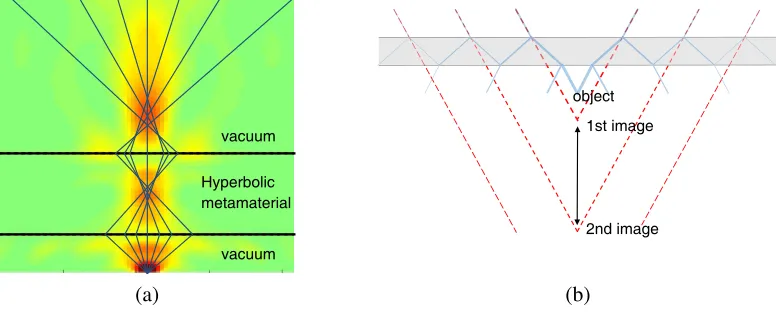
Figure 1. No unambiguous image distance can be determined from an intensity map due to aberration, (a) which results in a blurry spot and (b) internal reflections which result in ghost images.
homogenization [25–27] of the metamaterial and the determination of the dispersion relation. If the dispersion relation is known for all angles of incidence, the Transfer Matrix Method (TMM) can be applied [26, 28] to calculate the image.
The image position can be defined as the maximum of the intensity function; however, this may lead to a false description, since the metamaterial introduces aberration and ghost images. Aberration occurs when rays with different angles of propagation do not intersect each other in one point, which results in a blurry spot (see Fig. 1(a)). Ghost images are produced by non-negligible internal reflections (see Fig. 1(b)). As a result, the intensity maximum of the blurry spot cannot unambiguously define the image position: from some viewing angle the observer may observe a completely different image position, due to angle dependent refraction. This angle dependence cannot be neglected.
In this paper, we propose a method that combines the dispersion relation obtained from full wave simulation of a metamaterial unit cell, with the Transfer Matrix Method to provide an efficient calculation procedure for determining the angle dependent image position of a point source situated behind a metamaterial slab. Superposing the effects of point sources, the image of extended objects can also be calculated.
2. RETRIEVING THE EFFECTIVE PARAMETERS OF METAMATERIALS
Due to their sub-wavelength feature sizes, metamaterials can be described macroscopically as homogeneous materials and characterized with macroscopic material parameters such as magnetic permeability and electric permittivity or refractive index and wave impedance. These macroscopic parameters can be deduced from calculated or measured S-parameters of a metamaterial slab with finite thickness [29].
Metamaterials are generally anisotropic, i.e., their macroscopic parameters strongly depend on the angle of incidence, and hence no global material parameters can be assigned to them [25]. Nevertheless, effective parameters can be retrieved for each angle of incidence, and metamaterials can be characterized with angle dependent electromagnetic parameters. Metamaterials as any periodic structure can be described with dispersion relation, which relates the wavenumber of a plane wave propagating in the metamaterial to its frequency [26, 30]. In the following, a metamaterial slab situated parallel to thexy
plane of a Cartesian coordinate system with thickness din the z direction is considered. The normal wave number kz and generalized wave impedance ξ are extracted for plane waves with arbitrary angle of incidence and frequency, in order to calculate the dispersion relation of the metamaterial. The generalized wave impedance determines reflections on the boundaries, and it is defined as
ξ= εr
kz
kz0 (1)
calculation does not require high computational effort as the computations involve only one unit cell. FromS-parameters, generalized wave impedance is retrieved for all angle of incidence as
ξ(α) =± √
(1 +S11(α))2−S212 (α) (1−S11(α))2−S2
21(α)
(2)
where S21(α) is the complex transmittance and S11(α) the complex reflectance for a plane wave excitation with incident angle α. The sign of Eq. (2) is chosen to fulfill the passivity condition Re{ξ}>0 [27]. The normal wavenumber can be retrieved [27] for any angle of incidence as
kz(α) =
Im{ln(S21(α)/(1−S11(α)Γ))}+ 2mπ
d −ı
Re{ln(S21(α)/(1−S11(α)Γ))}
d , (3)
wherem is the branch number, dthe thickness of the slab,i=√−1, and Γ the reflection coefficient
Γ(α) = ξ(α)−1
ξ(α) + 1. (4)
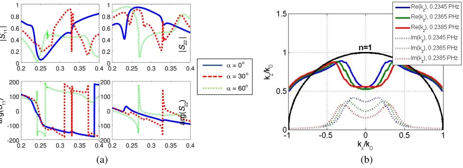
The lateral wavenumber kx is conserved at the interface of the metamaterial and its surrounding medium, and it is determined as kx = k0(sinα), assuming that the surrounding medium is vacuum, where k0 is the free-space wavenumber andα the angle of incidence. The relation between kz and kx yields the dispersion relation for any fixed frequency (see Fig. 2(b)).
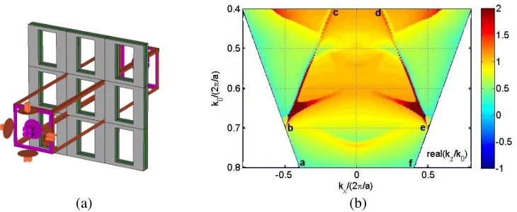
The procedure is applied to retrieve the dispersion relation of a fishnet type metamaterial working in the optical regime. The fishnet structure is a metal-insulator-metal structure with periodically arranged sub-wavelength sized rectangular holes in it, and the unit cell is shown in Fig. 3(a). The materials and geometric parameters are chosen as in [32]. The size of the rectangular unit cell is 600×600 nm. The size of the hole is 284×500 nm. The thickness of the MgF2 insulator layer is 30 nm, and the thickness of the metallic layers made of silver is 45 nm.
The homogenization procedure replaces the metamaterial slab with a homogeneous slab in such a way that the transmission and reflection parameters coincide. The thickness of the homogeneous layer is the effective thickness of the metamaterial, which is not necessarily equal to the thickness of the metal and insulator layers [29]. The effective thickness of the metamaterial is chosen to be 460 nm = 2×45 nm + 30 nm + 340 nm, where 340 nm represents an additional air region, which is the separation between the layers of the multilayer fishnet structure utilized in the next section of the paper.
(a) (b)
|
S
|
11
|
S
|
22
arg(
S
)
11
arg(
S
)
22
α = 0o
α = 30
α = 60 o
o
(a) (b)
Figure 3. (a) Nine unit cells of the investigated fishnet structure. (b) The full dispersion relation of the fishnet structure for TM mode.
Figure 2(a) shows the calculated S-parameters for TM illumination obtained from full-wave simulation performed with CST Microwave Studio. In Fig. 3(b), the TM dispersion relation of the fishnet metamaterial is presented. Inside the a-b-c-d-e-f polygon no higher diffraction orders are excited. Consequently, in this region the metamaterial can be homogenized.
In Fig. 2(b), the dispersion curves of the fishnet are compared to the dispersion curves of the vacuum for several frequencies. The figure reveals a highly anisotropic nature of the fishnet metamaterial. For small incident angles, the dispersion relation is hyperbolic, while for large incident angles, it is elliptic, which leads to strongly angle-dependent imaging behavior in this specific frequency region.
The calculation of S-parameters is performed with the Finite Element Solver of CST Microwave Studio, and it takes around 1 hour 10 minutes for 40 incident angles for a single frequency on Intel i5 processor.
3. THE IMAGE OF A POINT SOURCE PLACED BEHIND A METAMATERIAL SLAB
3.1. Intensity Map
The response of a linear imaging system to point sources fully characterizes its behavior. Therefore, in this section the electromagnetic field of a single point source placed behind a metamaterial slab is calculated, from which the intensity map is given as the square of the absolute value of the electric field. The EM field can be calculated with different methods, such as the FDTD (Finite Difference Time Domain) algorithm [33]. However, the FDTD method is memory and time consuming when subwavelength metallic structures such as metamaterials are simulated. Taking the advantage that the effective parameters are already known, the Transfer Matrix Method [16, 34] can provide a much more efficient simulation tool. We developed a modified formulation of the method, where the transfer function is calculated with the dispersion relation introduced in the previous section and illustrated for the fishnet type metamaterial in Fig. 2(b) and Fig. 3(b). The 2D calculations are performed in a configuration similar to [16], assuming that the metamaterial slab has an infinite extent in lateral directions. It is also assumed that TE and TM modes of the electromagnetic waves can be considered separately, and thus the electric or the magnetic field can be handled as a scalar field.
The point source is modeled with a thin slit in the source plane, thinner than the wavelength. Although this excitation does not yield the exact electromagnetic distribution of a point source, it excites all propagating spatial spectral components and has the advantage of having finite spectral components for all lateral frequencies. Spectral components that cannot propagate in vacuum can be neglected, since they will not reach the observer.
kxand with complex amplitudeHysrc(kx). The complex amplitude of each plane wave is then calculated in the image plane behind the metamaterial slab with the transfer function
Hyimg(kx) =T0,1(kx)Tslab(kx)T0,2(kx)Hysrc(kx). (5)
where the transfer function of the surrounding medium (vacuum) is
T0,j(kx) =eıkz0ds,j, j= 1,2, (6)
whereds,1 is the distance between the source plane and the metamaterial slab,ds,2 the distance between the metamaterial slab and the image plane and kz0 the normal wave number that corresponds to the lateral wave numberkxin vacuum. The transfer function (or transmission coefficient) of a homogeneous slab with finite thickness is
Tslab(kx) = 4
(ξ+ 1) (
1
ξ + 1
)
e−ıkzd+ (ξ−1) (
1
ξ −1
)
eıkzd
(7)
wheredis the thickness of the slab,ξ(kx) the generalized wave impedance and kz(kx) the normal wave number in the medium that corresponds to kx [16, 31]. This transfer function is calculated from the continuity conditions of the electromagnetic field components at the interfaces between different media and provides a steady state solution. The steady state solution is the sum of a directly transmitted wave and the waves that emerge from the medium after multiple internal reflections. To omit the effect of internal reflections within the metamaterial slab, the transfer function of the slab can be simplified to
Tslab(kx) = (1−Γ)eıkzd(1 + Γ), (8)
where Γ is the reflection coefficient. This transfer function considers direct, non-reflected wave only, which enters the medium (Γ is the proportion, which is lost due to reflection), propagates in the medium with normal wavenumber kz, and then emerges from the medium (−Γ is the proportion, which is lost due to reflection) [26].
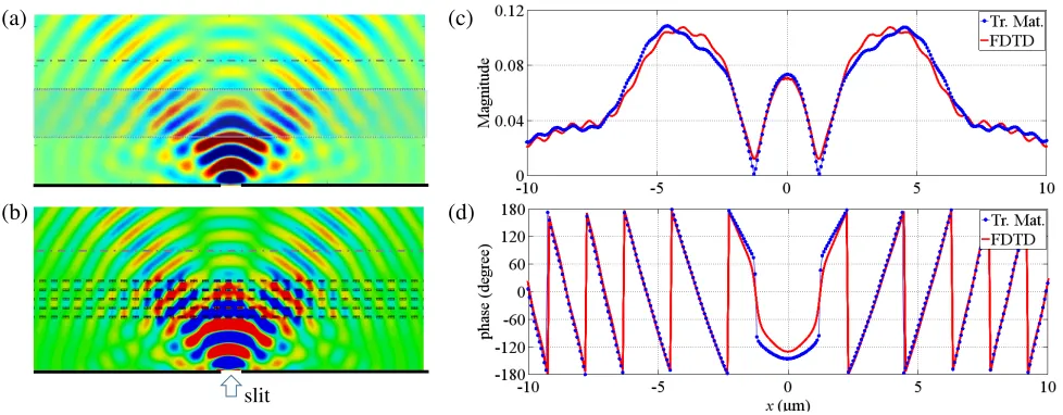
After the calculation of the complex amplitudesHyimg(kx) in the image plane, the contributions of each plane wave are summed up to provide the full electromagnetic field distribution in the image plane. Fig. 4(a) shows the electromagnetic field distribution computed with the Transfer Matrix Method using the dispersion relation of the fishnet metamaterial.
For comparison, Fig. 4(b) shows the electromagnetic field distribution computed with 3D FDTD simulation (CST Microwave Studio) which takes into account the fine details of the fishnet metamaterial. The FDTD simulations are performed for a 5-layered multilayer fishnet structure with 1 unit cell in the vertical direction parallel to the slit and 82 unit cells in the horizontal direction perpendicular to the slit. The FDTD computational space is truncated with PEC in the horizontal direction and PMC in the vertical direction to simulate an infinite structure, while the remaining faces, which are parallel to the multilayer fishnet are closed with perfectly matched layer [33]. The distance specified by the 82 cells (≈39λ) is large enough, that the neighboring sources introduced by the boundary conditions make small effect on the field distribution in front of the metamaterial. In the Transfer Matrix Method, the same simulation width is utilized, and Discreet Fourier Transform is applied, which introduces periodicity in the horizontal direction as well, making it possible to compare the two methods. Figs. 4(c) and (d) show the comparison of the amplitude and phase distributions along a line in front of the metamaterial slab calculated with the FDTD and the Transfer Matrix Method. The root mean square error of the phase along this line is 0.315 radians. The RMS error of the magnitude is 3.62e−3 (Amax= 0.109).
slit
(a)
(b)
(c)
(d)
Figure 4. The electromagnetic field distribution of the point source placed behind the metamaterial slab of 5 fishnet layers is calculated (a) with the Transfer Matrix Method and (b) with full 3D FDTD simulation. (c) The magnitude and (d) phase distributions calculated with the two methods are compared along the dashed gray lines of (a) and (b). The operating frequency is f = 0.2385 PHz. The simulation area is 82 unit cells wide, but only a 33 unit cells wide area is shown on each figure.
3.2. Observation Angle Dependent Image Distance
The electromagnetic field distribution in front of the metamaterial, as depicted in Figs. 4(a) and (b), conveys an impression of how the metamaterial distorts the wave fronts but does not provide the information and what an observer would see while observing the point source placed behind the metamaterial. The calculated intensity distribution would be observed only if all plane waves leaving the metamaterial could reach the observer. However, the observer perceives only those waves that propagate toward him. Consequently, to calculate the image distance seen by the observer, only a portion of the plane waves are summed, which can be simply achieved by modifying the last step of the Transfer Matrix Method. In our calculations, 1◦ wide angle range around the observation angle is considered.
The effect of internal reflections (i.e., ghost images) can also be simply eliminated with the Transfer Matrix Method applying (8) instead of Eq. (7) in the calculations [26]. If this transfer function is applied, only non-reflected waves are considered in the image plane, i.e., only the brightest image is observed.
After summing the plane waves reaching the observer, the position of the image for the given observation angle is found at the intensity maximum as shown in Figs. 5(a)–(d). This process is repeated for all observation angles. Fig. 5(e) shows the computed source-image distance in function of the observation angle. Due to the homogeneity of the slab, the source-image distance is independent of the source position, hence this parameter can fully characterize the metamaterial slab. Note that the image position strongly depends on the observation angle. Consequently, the intensity maximum of the field calculated with FDTD cannot be used to determine a correct image position.
Often the image produced by the metamaterial slab is behind the surface of the metamaterial. In this case, the intensity maximum cannot be found within the computational domain, hence the virtual image is determined by field reversal applying the inverse transfer function of vacuum
T0−1(kx) = exp(−ıkz0d) (9)
for the spatial spectral coefficients of the electromagnetic field in the image plane. Figs. 5(b) and 5(d) show the backward computed electric field/intensity distributions, when the intensity maximum is found behind the surface of the metamaterial.
(c) (d)
d
Source position = 0
Figure 5. The magnetic field distribution obtained by summing plane waves in the range of−12◦ . . . 12◦ and in the range of 40◦ . . .70◦ are shown in (a) and (b), while the intensity distributions for the same angle ranges are plotted in (c) and (d). These wide angle ranges are applied only for visualization purposes. In case of (e), which shows the computed image position with respect to the angle of observation, 1◦ wide angle ranges are considered, i.e., 0◦–1◦, 1◦–2◦,. . ., 59◦–60◦ to minimize the effect of aberration. The working frequency is f = 0.2385 PHz.
(a) (b)
Observer
image
object DFT of the source field
H y,src(k x)
T(k y) Transfer function
Calculate k (α) and ξ(α) from the S-parameters
i = i + 1 Transmitted plane waves
(α = 0 ... 90 ) o H y,img(k x)
Sum plane waves between [α i- ∆α ... α i+ ∆α]
(k x,i= k 0sinα i)
Find intensity maximum, store in F(α )
i
Plot F(α)
d
z F
dy
dx α
β
α
Figure 6. (a) Flowchart of the angle dependent image distance retrieving procedure. (b) Geometrical constraints between the image distance and the observation angle. The observation angle is determined by the image distance.
investigated fishnet structure. The strong angle dependence of the source-image distance is well seen in the figure. This cannot be revealed from a full intensity map.
Figure 6(a) concludes the whole process from the effective parameter retrieval to the determination of the angle dependent image distance.
4. THE IMAGE OF EXTENDED OBJECTS PLACED BEHIND A METAMATERIAL SLAB
of the extended object can be determined.
When the observer is far and the extended object seen under a small viewing angle, the image of the object can be found at distanceF from the object, whereF is the calculated source-image distance for the given observation angle.
However, when the observer is near the object, which is seen under a large viewing angle, the problem is more challenging, because the observation angleα of the point sources is unknown, until the image position of the point source is determined (see Fig. 6(b)). The image position, in turn, depends on the observation angle as discussed before and as can be seen in Fig. 5(e). Therefore, the image position can be determined by simultaneously satisfying both the geometrical constraints and the source-image distance vs. observation angle function F(α). The geometrical constraint between the source-image distanceF and the observation angleα for one point of the object can be derived based on Fig. 6(b) as
tanα=dx/(dy−F) (10)
where dx is the horizontal and dy the vertical distance between the observer and the point source. If
F(α) is known, then the image position can be obtained by the numerical solution of the equation
(dy−F(α)) tanα−dx= 0. (11)
Note that this nonlinear equation may have multiple solutions.
When the image distance is found, an effective refractive angleβcan also be introduced as depicted in Fig. 6(b) by satisfying the condition
ztanα+dtanβ+ (F −d−z) tanα = 0 (12)
where β is the effective refractive angle, α the angle of incidence, z the distance between the point source and the surface of the metamaterial,dthe thickness of the metamaterial andF the source-image distance. The effective refractive angle can be expressed as
tanβ = d−F
d tanα. (13)
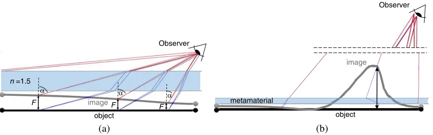
In the following, two examples demonstrate the applicability of the presented method. In the first one, the image of a rod placed behind a glass slab with constant refractive index is calculated. For this case, the source-image distance F(α) is calculated with Snell’s law as
F(α) =d−dtan(arcsin(1/nsin(α)))
tan(α) ; (14)
where n = 1.5 is the refractive index of the glass. Fig. 7(a) shows the calculated image of the rod placed behind the glass slab. From the figure it can be seen that the rod is virtually bent, similar to the bottom of a swimming pool when observed from the edge of the pool.
In the second example, the rod is placed behind the metamaterial slab with the dispersion relation presented in Fig. 2(b). The image of the rod is distorted as shown in Fig. 7(b). There is an angle range where the image floats in front the metamaterial slab, due to its partially hyperbolic dispersion
(a) (b)
Observer
image
object Observer
object
image metamaterial
n =1.5
α α
F F F
α
Although not depicted here, the intensity of the image also varies with the observation angle. This intensity function can be obtained along with the source-image distance function from the modified transfer function method.
5. CONCLUSION
We propose a method to describe the imaging properties of metamaterials. Instead of applying full-wave simulation for the whole structure, first we determine the dispersion relation with the simulation of one unit cell, then we apply the Transfer Matrix Method to calculate the image of a point source. The procedure can be utilized even for frequency ranges where the metamaterial cannot be homogenized and removes the burden of effective metamaterial parameter retrieval. Beside its effectiveness, the method has the ability to cancel the effect of internal reflections, to avoid ghost images and to deal with aberration, which is introduced by the greatly angle dependent properties of metamaterials. With this method, the image distance can be obtained as a function of the observation angle. Knowing the position of the image produced by the point source for all observation angles allows us to determine the image of extended objects as it is perceived by an observer even if it is seen under a wide viewing angle.
ACKNOWLEDGMENT
This work has been supported by the Bolyai Janos Fellowship of the Hungarian Academy of Sciences, PIAC-13-1-2013-0186 and KMR-12-1-2012-0008 of the National Development Agency Hungary and the EUREKA project MetaFer.
REFERENCES
1. Solymar, L. and E. Shamonina, Waves in Metamaterials, Oxford University Press, 2009.
2. Pendry, J. B., “Negative refraction makes a perfect lens,” Physical Review Letters, Vol. 85, 3966– 3969, 2000.
3. Shelby, R. A., D. R. Smith, and S. Schultz, “Experimental verification of a negative index of refraction,” Science, Vol. 292, No. 5514, 77–79, 2001.
4. Smith, D. R., J. B. Pendry, and M. C. K. Wiltshire, “Metamaterials and negative refractive index,” Science, Vol. 305, No. 5685, 788–792, 2004.
5. Shalaev, V. M., “Optical negative-index metamaterials,” Nature Photonics, Vol. 1, 41–48, 2007. 6. Moitra, P., Y. Yang, Z. Anderson, I. I. Kravchenko, D. P. Briggs, and J. Valentine, “Realization of
an all-dielectric zero-index optical metamaterial,” Nature Photonics, Vol. 7, 791–795, 2013. 7. Choi, M., S. H. Lee, Y. Kim, S. B. Kang, J. Shin, M. H. Kwak, K.-Y. Kang, Y.-H. Lee, N. Park,
and B. Min, “A terahertz metamaterial with unnaturally high refractive index,”Nature, Vol. 470, No. 7334, 369–373, 2011.
8. Ziolkowski, R. W., “Design, fabrication, and testing of double negative metamaterials,” IEEE Transactions on Antennas and Propagation, Vol. 51, 1516–1529, 2003.
9. Shalaev, V. M., W. Cai, U. K. Chettiar, H.-K. Yuan, A. K. Sarychev, V. P. Drachev, and A. V. Kildishev, “Negative index of refraction in optical metamaterials,” Optics Letters, Vol. 30, No. 24, 3356–3358, 2005.
10. Cai, W. and V. M. Shalaev,Optical Metamaterials, Springer, 2010.
11. Kildishev, A. V., A. Boltasseva, and V. M. Shalaev, “Planar photonics with metasurfaces,”Science, Vol. 339, 1232009, 2013.
13. Belov, P. and Y. Hao, “Subwavelength imaging at optical frequencies using a transmission device formed by a periodic layered metal-dielectric structure operating in the canalization regime,” Physical Review B — Condensed Matter and Materials Physics, Vol. 73, No. 11, 113110, 2006. 14. Hegde, R. S., Z. Szab´o, Y. L. Hor, Y. Kiasat, E. P. Li, and W. J. R. Hoefer, “The dynamics of
nanoscale superresolution imaging with the superlens,” IEEE Transactions on Microwave Theory and Techniques, Vol. 59, 2612–2623, 2011.
15. Lu, D. and Z. Liu, “Hyperlenses and metalenses for far-field super-resolution imaging,” Nature Communications, Vol. 3, 1205, 2012.
16. Szab´o, Z., Y. Kiasat, and E. P. Li, “Subwavelength imaging with composite metamaterials,”Journal of the Optical Society of America B — Optical Physics, Vol. 31, No. 6, 1298–1307, 2014.
17. Aieta, F., P. Genevet, M. A. Kats, N. Yu, R. Blanchard, Z. Gahurro, F. Capasso, Z. Gaburro, and F. Capasso, “Aberration-free ultrathin at lenses and axicons at telecom wavelengths based on plasmonic metasurfaces,”Nano Letters, Vol. 12, No. 9, 4932–4936, 2012.
18. Aieta, F., P. Genevet, M. Kats, and F. Capasso, “Aberrations of at lenses and aplanatic metasurfaces,” Optics Express, Vol. 21, 31530–31539, 2013.
19. Luo, C., S. G. Johnson, J. D. Joannopoulos, and J. B. Pendry, “All-angle negative refraction without negative effective index,”Physical Review B, Vol. 65, No. 20, 201104, 2002.
20. Lu, W. T. and S. Sridhar, “Flat lens without optical axis: Theory of imaging,” Optics Express, Vol. 13, No. 26, 10673–10680, 2005.
21. Fan, X., G. P. Wang, J. C. W. Lee, and C. T. Chan, “All-angle broadband negative refraction of metal waveguide arrays in the visible range: Theoretical analysis and numerical demonstration,” Physical Review Letters, Vol. 97, No. 7, 1–4, 2006.
22. Lu, W. T. and S. Sridhar, “Superlens imaging theory for anisotropic nanostructured metamaterials
with broadband all-angle negative refraction,” Physical Review B — Condensed Matter and
Materials Physics, Vol. 77, No. 23, 1–4, 2008.
23. Yao, J., K.-T. Tsai, Y. Wang, Z. Liu, G. Bartal, Y.-L. Wang, and X. Zhang, “Imaging visible light using anisotropic metamaterial slab lens,” Optics Express, Vol. 17, 22380–22385, 2009.
24. Silin, R., “On the history of backward electromagnetic waves in metamaterials,” Metamaterials, Vol. 6, No. 1–2, 1–7, 2012.
25. Menzel, C., C. Rockstuhl, T. Paul, F. Lederer, and T. Pertsch, “Retrieving effective parameters for metamaterials at oblique incidence,”Physical Review B, Vol. 77, 195328, 2008.
26. Paul, T., C. Rockstuhl, C. Menzel, and F. Lederer, “Anomalous refraction, diffraction, and imaging in metamaterials,”Physical Review B, Vol. 79, No. 11, 115430, 2009.
27. Szab´o, Z., G.-H. H. Park, R. Hedge, and E. P. Li, “A unique extraction of metamaterial parameters based on Kramers-Kronig relationship,”IEEE Transactions on Microwave Theory and Techniques, Vol. 58, No. 10, 2646–2653, 2010.
28. Szab´o, Z. and J. F¨uzi, “Equivalence of magnetic metamaterials and composites in the view of effective medium theories,” IEEE Transactions on Magnetics, Vol. 50, No. 4, 1–4, 2014.
29. Chen, X. D., T. M. Grzegorczyk, B. I. Wu, J. Pacheco, and J. A. Kong, “Robust method to retrieve the constitutive effective parameters of metamaterials,”Physical Review E, Vol. 70, No. 1, 016608, 2004.
30. Brillouin, L., Wave Propagation in Periodic Structures: Electric Filters and Crystal Lattices, Courier Corporation, 2003.
31. Bohren, C. F. and D. R. Huffman, Absorption and Scattering of Light by Small Particles, John Wiley & Sons, 2008.
32. Dolling, G., C. Enkrich, M. Wegener, C. M. Soukoulis, and S. Linden, “Low-loss negative-index metamaterial at telecommunication wavelengths,”Optics Letters, Vol. 31, 1800–1802, 2006. 33. Taflove, A. and S. C. Hagness, Computational Electrodynamics, Artech House Publishers, 2000. 34. Born, M. and E. Wolf, Principles of Optics: Electromagnetic Theory of Propagation, Interference