Array Aperture Extension Algorithm for 2-D DOA Estimation
with L-Shaped Array
Xi Nie* and Ping Wei
Abstract—In this paper, an array aperture extension algorithm is developed for two-dimensional (2-D) direction-of-arrival (DOA) estimation with L-shaped array. We enlarge the dimension of the covariance matrix by using the rotational invariance in conjunction with the property that the signal covariance matrix is real diagonal matrix. Estimation of DOAs is performed by processing this larger dimensional matrix. The simulation results indicate that our method can improve the DOA estimation accuracy.
1. INTRODUCTION
Estimation of two-dimensional (2-D) direction of arrival (DOA) of multiple incident signals using sensor array techniques has attracted considerable attention in many applications including radar, sonar, wireless communication, and seismic sensing [1], and lots of high-resolution algorithms were proposed in literatures [2–6] in the past decade. Most of the above-mentioned approaches directly deal with the covariance matrix of the received signals to estimate the DOAs of the signal sources. In this paper, we introduce a method to enlarge the dimension of the covariance matrix with L-shaped array. Our method extends the dimension of the covariance matrix by employing the rotational invariance and the property that the covariance matrix of the signal sources is real diagonal matrix. Then, the signal DOAs are found by processing the larger dimensional matrix. Computer simulations show that the proposed approach can obtain good DOA estimation performance.
Notations: The superscript ∗, T, H, and † denote the conjugate, the transpose, the conjugate transpose, and Moore-Penrose inverse respectively. E{·}, J, and M[i : j,:] stand for the statistical expectation, an exchange matrix with ones on its antidiagonal and zeros elsewhere, and a matrix consisting of theith tojth rows of matrixM respectively.
2. DATA MODEL
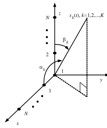
Consider K narrowband far-field plane signals {sk(t)}Kk=1 from distinct directions impinging on an
L-shaped array composed of two uniform linear arrays (ULAs) alongxandzaxes respectively. Each ULA consists of N isotropic sensors, and the inter-sensor spacing d along x and z axes is half-wavelength
λ/2. Letαk andβk,k= 1,2, . . . , K, be the azimuth and elevation angles of thekth source. Note that
the azimuth angle αk is taken between the signal arrival direction and x axis, and the elevation angle βk is taken between signal arrival direction and zaxis, as shown in Figure 1.
The array manifold matrices can be given as
A(α) = [a(α1),a(α2), . . . ,a(αK)] (1)
A(β) = [a(β1),a(β2), . . . ,a(βK)] (2)
wherea(αk) = [1, ξk, . . . , ξkN−1]T,ξk=ejπcosαk,a(βk) = [1, ηk, . . . , ηNk−1]T,ηk =ejπcosβk.
Received 15 January 2015, Accepted 6 March 2015, Scheduled 16 March 2015 * Corresponding author: Xi Nie ([email protected]).
x
y z
1
k
s (t), k=1,2,...,K
N
1
N
2
k k
β
α
..
.
.
.
.
Figure 1. L-shaped array configuration for 2-D DOA estimation.
The observed vectorsx(t) andz(t) can be written as
x(t) =A(α)s(t) +nx(t) (3) z(t) =A(β)s(t) +nz(t) (4)
where x(t) = [x1(t), x2(t), . . . , xN(t)]T,z(t) = [z1(t), z2(t), . . . , zN(t)]T,s(t) = [s1(t), s2(t), . . . , sK(t)]T,
nx(t) = [nx1(t), nx2(t), . . . , nxN(t)]T,nz(t) = [nz1(t), nz2(t), . . . , nzN(t)]T. s(t) is a K×1 source vector,
and nx(t) and nz(t) are additive noise in the x and z axes subarrays, respectively. Assume that the sources are uncorrelated with each other, and the noise is a white Gaussian random processes with zero-mean and varianceσ2, and is statistically independent of signal samples.
3. PROPOSED ALGORITHM
From the above assumption, we calculate the covariance matrix of the observations as
Rxz =Ex(t)zH(t)=A(α)Es(t)sH(t)AH(β) +Enx(t)nHz (t)=A(α)RsAH(β) (5) where the diagonal matrix Rs = diag{p1, p2, . . . , pK} is the signal covariance matrix, and positive real
number pk stands for the power of the kth signal source. Note that nx(t) and nz(t) are spatially
independent of each other, i.e.,E{nx(t)nHz (t)}=0.
3.1. Covariance Matrix for Signal Subspace Identification
Performing the singular value decomposition (SVD) of Rxz
Rxz =A(α)RsAH(β) =UΣVH (6) where Σ = diag(d1, d2, . . . , dK) with d1 ≥ d2 ≥ . . . ≥ dK > 0, d1, d2, . . . , dK stand for the K largest
singular values of Rxz,U and V stand for the left and right singular vectors of Rxz corresponding to
K largest singular values, respectively.
It is well known that the K columns of U and A(α) span the same range space. Therefore, there exists an invertible matrix W1 such that
U=A(α)W1. (7)
DivideUinto two (N−1)×KmatricesU1andU2such thatU1 =U[1 :N−1, :],U2 =U[2 :N,:].
Accordingly, U1 and U2 can be represented as
U1=A1(α)W1 (8)
whereA1(α) =A(α)[1 :N−1,:],A2(α) =A(α)[2 :N,:].
According to the rotational invariance, we have
A2(α) =A1(α)Dα (10)
whereDα is a diagonal matrix with Dα= diag(ξ1, ξ2, . . . , ξK).
Combining (7), (8), (9) with (10), we get
U
U†2U1 N
=A(α)W1
W1−1A†2(α)A1(α)W1 N
=A(α)D−αNW1 =Anew1(α)W1 (11)
whereAnew1(α) = [anew1(α1),anew1(α2), . . . ,anew1(αK)], anew1(αk) = [ξ−kN, ξk−(N−1), . . . , ξk−1]T.
Substituting (7) into (6), we obtain
RsAH(β) =W1ΣVH. (12)
We define the first matrixR12 as
R12 U
U†2U1 N
ΣVH. (13)
According to (11) and (12),R12 can be rewritten as
R12=Anew1(α)RsAH(β). (14)
Likewise, the K columns of V and A(β) span the same range space. There exists an invertible matrixW2 satisfied the following equality
V=A(β)W2. (15)
DivideVinto two (N−1)×K matricesV1andV2such thatV1 =V[1 :N−1,:],V2 =V[2 :N,:].
Accordingly, V1 and V2 can be represented as
V1=A1(β)W2 (16)
V2=A2(β)W2 (17)
whereA1(β) =A(β)[1 :N−1,:],A2(β) =A(β)[2 :N,:].
By means of the rotational invariance, we obtain
A2(β) =A1(β)Dβ (18)
whereDβ is also a diagonal matrix with Dβ = diag(η1, η2, . . . , ηK).
Combining (15), (16), (17) with (18), we have
V
V†2V1 N
=A(β)W2
W2−1A†2(β)A1(β)W2 N
=A(β)D−βNW2 =Anew1(β)W2 (19)
whereAnew1(β) = [anew1(β1),anew1(β2), . . . ,anew1(βK)],anew1(αk) =
ηk−N, ηk−(N−1), . . . , η−k1]T. Substituting (15) into (6), we get
A(α)Rs =UΣWH2 . (20)
We define the second matrixR21as
R21UΣ
V
V†2V1 NH
. (21)
From (19) and (20),R21 can be rewritten as
R21=A(α)RsAHnew1(β). (22)
Next, we define the third matrixR11 as
R11J
UU†1U2Σ
VV†1V2 H∗
According to (6), (7), (8), (9), (10), (15), (16), (17) and (18), R11 can be expressed as
R11=J
A(α)DαW1Σ(A(β)DβW2)H ∗
J=Anew1(α)Rs∗AHnew1(β). (24)
SinceRs is real diagonal matrix, the equality Rs=R∗s holds. Thus,R11 can be represented as
R11=Anew1(α)RsAHnew1(β). (25)
CombiningR11,R12,R21 withRxz, we construct a new matrixRnew
Rnew = RR11 R12
21 Rxz
(26)
According to (5), (14), (22) and (25), Rnew can be expressed as
Rnew = Anew1(α) A(α)
Rs Anew1(β) A(β)
H
=Anew(α)RsAHnew(β) (27)
where Anew(α) = [anew(α1),anew(α2), . . . ,anew(αK)], anew1(αk) = [ξk−N, ξk−(N−1), . . . , ξk−1,1, ξk1, . . ., ξk(N−1)]T, Anew(β) = [anew(β1),anew(β2), . . . ,anew(βK)], anew(βk) = [ηk−N, ηk−(N−1), . . . , ηk−1,1, η1k, . . ., ηk(N−1)]T.
It is evident that Anew(α) and Anew(β) correspond to an array manifold matrix of a ULA with 2N array elements andRnew corresponds to a covariance matrix of a cross-array with 2N + 2N array elements, which indicates that the number of array elements increases fromN +N to 2N+ 2N.
3.2. Estimation of the Azimuth α and the Elevation β
Performing the SVD of Rnew
Rnew =Anew(α)RsAnewH (β) =UΣVH (28)
where Σ = diag(d1,d2, . . . , dK) with d1 ≥ d2 ≥ . . . ≥ dK > 0, d1, d2, . . . , dK stand for the K largest
singular values ofRnew,U and V stand for the left and right singular vectors of Rnew corresponding to theK largest singular values, respectively.
Next, we define three matrices Σ, U and V as ΣΣ1/2, U UΣ and V VΣ. Accordingly, (28) could be rewritten as
Anew(α)RsAHnew(β) =UVH. (29)
We have known that U and Anew(α) span the same range space, and V and Anew(β) span the same range space. Hence, the following two equalities hold
Anew(α) =UP1 (30)
Anew(β) =VP2 (31)
whereP1 and P2 are two invertible matrices.
Then, we can utilize the conventional ESPRIT procedure [7] to estimate the azimuth αk and the
elevation βk. Divide U into two (2N −1)×K matrices U1 and U2 such that U1 = U[1 : 2N −1,:],
U2 =U[2 : 2N,:].
Performing the eigenvalue decomposition (EVD) of U†1U2, the eigenvectors P1 of U†1U2 must
satisfy the following equality
P1 =P1C1 (32)
whereC1is a permutation matrix composed of a single nonzero constant along every row or column and
zeros elsewhere. The eigenvalues λαk of U†1U2 must be equal toejπcosαk,k= 1,2, . . . , K. Accordingly,
the azimuthαk, k= 1,2, . . . , K, could be obtained by solving the following nonlinear equation
αk= cos−1 arg(λαk)
π
Similarly, performing the EVD of V†1V2, where V1 = V[1 : 2N −1,:], V2 = V[2 : 2N,:]. The
eigenvectors P2 of V†1V2 must satisfy the following equality
P2 =P2C2 (34)
where C2 is also a permutation matrix. The eigenvalues λβk of V1†V2 must be equal to ejπcosβk, k= 1,2, . . . , K. The elevationβk,k= 1,2, . . . , K, could be obtained by solving the following nonlinear equation
βk= cos−1 arg(πλβk)
k= 1,2, . . . , K. (35)
3.3. Pair Matching
Combining (29), (30) with (31), we have [8]
PH1 P2=R−s1. (36)
SinceRs is a diagonal matrix,R−s1 is also a diagonal matrix. We define a matrixPas
PP1HP2. (37)
According to (32), (34) and (36),Pcan be represented as
P=CH1 PH1 P2C2 =CH1 R−s1C2. (38)
SinceC1andC2 are two permutation matrix andR−s1is a diagonal matrix,Pis also a permutation
matrix. (38) implies that if the eigenvectors of U†1U2 and V†1V2 are unit vectors, only one element
value is close to 1 for every row or column inP. We can pair 2-D angles of the signals by utilizing this property. Let the eigenvectors of U†1U2 and V†1V2 be unit vectors, if pi,j is close to 1, theith azimuth
and jth elevation angles come from a couple of incident angles, where pi,j denotes the element value of theith rowjth column inP.
4. COMPUTATIONAL COMPLEXITY
In this section, we analyse the computational complexity of the proposed method. From the derivation of the presented method, we can see that the computational complexity of our method mainly focuses on two SVD. One is to perform the SVD of a N ×N matrix, and the computational cost is 24N3+ 48N3+ 54N3= 126N3 flops [10]. The other is to perform the SVD of a 2N×2N matrix, and the computational burden is 24(2N)3+ 48(2N)3+ 54(2N)3 = 1008N3. Since our method need to deal with a larger dimensional matrix, the computational cost of our method increases somewhat. However, our method can enhance the DOA estimation accuracy, and the simulation would verify this conclusion in the next section.
5. SIMULATION RESULTS
In this section, we illustrate the performance of our method by simulations. We compare our method with CCM-ESPRIT in [2], JSVD in [3] and Cramer Rao bound (CRB) in [9]. An L-shaped array is employed with 8 sensors for each ULA. The elements of each antenna array are separated by a half-wavelength. For simplicity, we suppose that all signal sources are of equal powerσs2, and the input SNR is defined as 10log10(σ2s/σn2). Define the root-mean-square-error (RMSE) of the DOA estimates fromN
Monte Carlo trials as
RMSE =
1
N K N
n=1 K
k=1
ˆ
α(kn)−αk 2
+
ˆ
βk(n)−βk 2
where ˆα(kn) and ˆβk(n) are the estimates of αk and βk for the nth Monte Carlo trial respectively, and K
is the source number.
In the first simulation, we examine the estimation performance of three methods in terms of SNR. Three signal directions are set to [α1, α2,α3] = [100◦,90◦,80◦], and [β1, β2, β3] = [70◦,80◦,90◦]. The
snapshot number is fixed at 500. The SNR varies from 0 dB to 15 dB.
In the second simulation, we research the RMSE of three methods with respect to the snapshot number. The incident directions of three sources are set to [α1, α2, α3] = [120◦,110◦,100◦] and
[β1, β2, β3] = [100◦,110◦,90◦]. The SNR is fixed at 5 dB. The snapshot number ranges from 200 to 2000.
From Figure 2 and Figure 3, it can be observed that our method is superior to CCM-ESPRIT and JSVD in different SNR and the snapshot number. It is because that our method utilizes the information Rs =R∗s to estimate the DOAs of signal sources, while CCM-ESPRIT and JSVD do not utilize this information.
In the third simulation, we investigate the estimation accuracy of the azimuth angles of three methods for different SNR. Three signal directions are set to [α1, α2, α3] = [60◦,70◦,80◦], and
[β1, β2, β3] = [110◦,120◦,130◦]. The snapshot number is fixed at 500. The SNR varies from 0 dB
to 15 dB.
0 5 10 15
SNR (dB) CCM-ESPRIT JSVD Our method CRB 0 0.1 0.2 0.3 0.4 0.5 0.6 0.7 RMSE (deg)
Figure 2. RMSE versus the SNR for 500 snapshots.
200 400 600 800 1000 1200 1400 1600 1800 2000 The snapshot number
CCM-ESPRIT JSVD Our method CRB 0.05 0.1 0.15 0.2 0.25 0.3 0.35 0.4 0.45 0.5 0.55 RMSE (deg)
Figure 3. RMSE versus the snapshot number, SNR = 5 dB.
0 5 10 15
SNR (dB) CCM-ESPRIT JSVD Our method 0.05 0.1 0.15 0.2 0.25 0.3 0.35 0.4 0.45 0.5 0.55
RMSE of azimuth angles (deg)
Figure 4. RMSE of azimuth angles versus the SNR for 500 snapshots.
0 5 10 15
SNR (dB) CCM-ESPRIT JSVD Our method 0 0.1 0.2 0.3 0.4 0.5 0.6 0.7
RMSE of elevation angles (deg)
In the fourth simulation, we test the estimation accuracy of the elevation angles of three methods for different SNR. The simulation condition is the same as the third one.
From Figure 4 and Figure 5, we can see that the DOA estimation accuracy of azimuth angles and azimuth angles is improved respectively by using our array aperture extension algorithm. The reason for this is that our method exploits more information to detect the DOAs of the signal sources.
6. CONCLUSION
This paper proposes an array aperture extension algorithm for 2-D DOA estimation with L-shaped array. Our method exploits rotational invariance, as well as the property that the signal covariance matrix is real diagonal matrix to construct a larger dimensional covariance matrix corresponding to a cross-shaped array with more array sensors. It is equal to enlarging the array aperture. Thus, our method achieves higher DOA estimation accuracy. Simulation results confirm the validity of the proposed method.
REFERENCES
1. Krim, H. and M. Viberg, “Two decades of array signal processing research,” IEEE Signal Process. Mag., Vol. 13, No. 4, 67–94, 1996.
2. Kikuchi, S., H. Tsuji, and A. Sano, “Pair-matching method for estimating 2-D angle with a cross-correlation matrix,” IEEE Antennas Wireless Propag. Lett., Vol. 5, 35–40, 2006.
3. Gu, J. F. and P. Wei, “Joint SVD of two cross-correlation matrices to achieve automatic pairing in 2-D angle estimation problems,”IEEE Antennas Wireless Propag. Lett., Vol. 6, 553–556, 2007. 4. Liang, J. L. and D. Liu, “Two L-shaped array-based 2-D DOAs estimation in the presence of mutual
coupling,”Progress In Electromagnetics Research, Vol. 112, 273–298, 2011.
5. Nie, X. and L. P. Li, “A computationally efficient subspace algorithm for 2-D DOA estimation with L-shaped array,” IEEE Signal Process. Lett., Vol. 21, No. 8, 971–974, 2014.
6. Albagory, Y. A., “Performance of 2-D DOA estimation for stratospheric platforms communica-tions,” Progress In Electromagnetics Research M, Vol. 36, 109–116, 2014.
7. Roy, R. and T. Kailath, “ESPRIT — Estimation of signal parameters via rotational invariance techniques,” IEEE Trans. Acoust., Speech, Signal Process., Vol. 37, No. 7, 984–995, 1989.
8. Nie, X. and L. P. Li, “A novel 2-D pair-matching algorithm using the special relation between the transition matrices and the autocorrelation matrix of the signals,” 2013 International Conference on Communications, Circuits and Systems (ICCCAS), 265–268, 2013.
9. Stoica, P. and A. Nehorai, “Performance study of conditional and unconditional direction-of-arrival estimation,” IEEE Trans. Acoust., Speech, Signal Process., Vol. 38, No. 10, 1783–1795, 1990. 10. Golub, G. H. and C. F. Van Loan,Matrix Computations, 3rd Edition, The John Hopkins University