Integral Cryptanalysis on Full MISTY1

Yosuke Todo

NTT Secure Platform Laboratories, Tokyo, Japan

[email protected]

Abstract. MISTY1 is a block cipher designed by Matsui in 1997. It was well evaluated

and standardized by projects, such as CRYPTREC, ISO/IEC, and NESSIE. In this paper, we propose a key recovery attack on the full MISTY1, i.e., we show that 8-round MISTY1 with 5 FL layers does not have 128-bit security. Many attacks against MISTY1 have been proposed, but there is no attack against the full MISTY1. Therefore, our attack is the first cryptanalysis against the full MISTY1. We construct a new integral characteristic by using the propagation characteristic of the division property, which was proposed in 2015. We first improve the division property by optimizing a public S-box and then construct a 6-round integral characteristic on MISTY1. Finally, we recover the secret key of the full MISTY1 with 263.58_{chosen plaintexts and 2}121 _{time complexity. Moreover, if we can use 2}63.994 _chosen plaintexts, the time complexity for our attack is reduced to 2107.9. Note that our cryptanalysis is a theoretical attack. Therefore, the practical use of MISTY1 will not be affected by our attack.

Keywords: MISTY1, Integral attack, Division property

1 Introduction

MISTY [Mat97] is a block cipher designed by Matsui in 1997 and is based on the theory of provable security [Nyb94,NK95] against differential attack [BS90] and linear attack [Mat93]. MISTY has a recursive structure, and the component function has a unique structure, the so-called MISTY structure [Mat96]. There are two types of MISTY, MISTY1 and MISTY2. MISTY1 adopts the Feistel structure whose F-function is designed by the recursive MISTY structure. MISTY2 does not adopt the Feistel structure and uses only the MISTY structure. Both ciphers achieve provable security against differential and linear attacks. MISTY1 is designed for practical use, and MISTY2 is designed for experimental use.

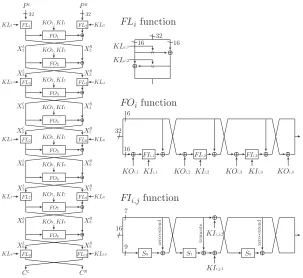
MISTY1 is a 64-bit block cipher with 128-bit security, and it has a Feistel structure with FL layers, where the F O function is used in the F-function of the Feistel structure.

The F O function is constructed by using the 3-round MISTY structure, where the F I

function is used as the F-function of the MISTY structure. Moreover, the F I function is constructed by using the 3-round MISTY structure, where a 9-bit S-box S9 and 7-bit

S-box S7 are used in the F-function. MISTY1 is the candidate recommended ciphers list

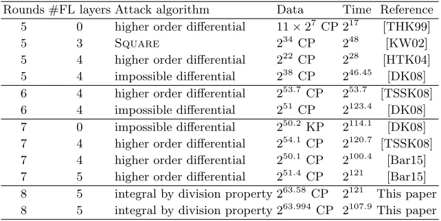
of CRYPTREC [CRY13], and it is standardized by ISO/IEC 18033-3 [ISO05]. Moreover, it is a NESSIE-recommended cipher [NES04] and is described in RFC 2994 [OM00]. There are many existing attacks against MISTY1, and we summarize these attacks in Table 1. A higher-order differential attack is the most powerful attack against MISTY1, and this type of cryptanalysis was recently improved in [Bar15]. However, there is no attack against the full MISTY1, i.e., 8-round MISTY1 with 5 FL layers.

?_c

Table 1.Summary of single secret-key attacks against MISTY1

Rounds #FL layers Attack algorithm Data Time Reference

5 0 higher order differential 11×27CP 217 [THK99]

5 3 Square 234CP 248 [KW02]

5 4 higher order differential 222_{CP 2}28 _[HTK04]

5 4 impossible differential 238_{CP 2}46.45 _[DK08]

6 4 higher order differential 253.7 CP 253.7 [TSSK08]

6 4 impossible differential 251CP 2123.4 [DK08]

7 0 impossible differential 250.2 KP 2114.1 [DK08] 7 4 higher order differential 254.1 CP 2120.7 [TSSK08] 7 4 higher order differential 250.1 CP 2100.4 [Bar15] 7 5 higher order differential 251.4 CP 2121 [Bar15] 8 5 integral by division property 263.58CP 2121 This paper 8 5 integral by division property 263.994 CP 2107.9This paper

Integral Attack The integral attack [KW02] was first proposed by Daemen et al. to

eval-uate the security of Square[DKR97] and was then formalized by Knudsen and Wagner.

There are two major techniques to construct an integral characteristic; one uses the prop-agation characteristic of integral properties [KW02], and the other estimates the algebraic degree [Knu94,Lai94]. We often call the second technique a “higher-order differential at-tack.” A new technique to construct integral characteristics was proposed in 2015 [Tod15], and it introduced a new property, the so-called “division property,” by generalizing the inte-gral property [KW02]. It showed the propagation characteristic of the division property for any secret function restricted by an algebraic degree. As a result, several improved results were reported on the structural evaluation of the Feistel network and SPN.

Our Contribution In [Tod15], the focus is only on the secret S-box restricted by an al-gebraic degree. However, many realistic block ciphers use more efficient structures, e.g., a public S-box and a key addition. In this paper, we show that the division property becomes more useful if an S-box is a public function. Then, we apply our technique to the cryptanal-ysis on MISTY1. We first evaluate the propagation characteristic of the division property for public S-boxes S7 and S9 and show that S7 has a vulnerable property. We next

eval-uate the propagation characteristic of the division property for the F I function and then evaluate that for theF O function. Moreover, we evaluate that for the FL layer. Finally, we create an algorithm to search for integral characteristics on MISTY1 by assembling these propagation characteristics. As a result, we can construct a new 6-round integral charac-teristic, where the left 7-bit value of the output is balanced. We recover the round key by using the partial-sum technique [FKL+_{00]. As a result, the secret key of the full MISTY1}

can be recovered with 263.58 _{chosen plaintexts and 2}121 _{time complexity. Moreover, if we}

can use 263.994 _{chosen plaintexts, the time complexity is reduced to 2}107.9_{. Unfortunately,}

we have to use almost all chosen plaintexts, and recovering the secret key by using fewer chosen plaintexts is left as an open problem.

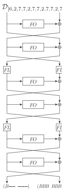
2 MISTY1

FL1

FO1

FO2

FL2

KO1,KI1

KO2, KI2

KL1 KL2

FO3

FO4

FL4

KO3,KI3

KO4,KI4

KL3 KL4

FO5

FO6

FL6

KO5,KI5

KO6,KI6

KL5 KL6

FL9

FO7

FO8

FL8

KO7, KI7

KO8,KI8

KL7 KL8

FL10

KL9 KL10 32 32

FO_i function FLi function

FI_i,j function

PL _PR

CL _CR X2L XR2

X3L XR3

XL4 XR4

XL5 XR5

X6L XR6

X7L XR7

X8L XR8

X9L XR9

FL3

FL5

FL7

Fig. 1.Specification of MISTY1

Let XL

i (resp. XiR) be the left half (resp. the right half) of an i-round input. Moreover,

XL

i [j] (resp.XiR[j]) denotes thejth bit ofXiL(resp.XiR) from the left. MISTY1 is a 64-bit block cipher, and the key-bit length is 128 bits. The component function F Oi consists of

F Ii,1,F Ii,2, andF Ii,3, and the four 16-bit round keys KOi,1,KOi,2,KOi,3, andKOi,4 are

used. The functionF Ii,j consists ofS9andS7, and a 16-bit round keyKIi,j is used. Here,S9

andS7are defined in Appendix A. The component functionF Li uses two 16-bit round keys,

KLi,1 andKLi,2. These round keys are calculated from the secret key (K1, K2, . . . , K8) as

Symbol KOi,1KOi,2KOi,3KOi,4KIi,1KIi,2KIi,3 KLi,1 KLi,2

Key Ki Ki+2 Ki+7 Ki+4 Ki0+5 Ki0+1 Ki0+3 Ki+1

2 (oddi) K

0

i+1 2 +6

(oddi)

K0

i

2+2

(eveni) Ki

2+4 (eveni)

Here,K0

i is the output of F Ii,j where the input isKi and the key isKi+1.

3 Integral Characteristic by Division Property

3.1 Notations

We make the distinction between the addition of Fn2 and addition of Z, and we use⊕ and

+ as the addition ofFn2 and addition of Z, respectively. For anya∈Fn2, the ith element is

expressed ina[i], and the Hamming weightw(a) is calculated asw(a) =Pn

i=1a[i]. Moreover,

a[i, . . . , j] denotes a bit string whose elements are values described into square brackets. Let 1n _∈

Fn2 be a value whose all elements are 1. Moreover, let 0n ∈ Fn2 be a value whose all

For any a∈(Fn21×F

n2

2 × · · · ×F

nm

2 ), the vectorial Hamming weight of a is defined as

W(a) = (w(a1), w(a2), . . . , w(am))∈Zm. Moreover, for anyk∈Zmandk0∈Zm, we define

kk0 ifki ≥k0i for all i. Otherwise, kk0.

Boolean Function A Boolean function is a function from Fn2 to F2. Let deg(f) be the

algebraic degree of a Boolean function f. Algebraic Normal Form (ANF) is often used as representations of the Boolean function. Letf be any Boolean function from Fn2 toF2, and

it can be represented as

f(x) = M u∈Fn2

af_u

n

Y

i=1

x[i]u[i]

!

,

where afu ∈ F2 is a constant value depending on f and u. If deg(f) is at most d, all afu satisfying d < w(u) are 0. An n-bit S-box can be regarded as the collection of n Boolean functions. If algebraic degrees of n Boolean functions are at most d, we say the algebraic degree of the S-box is at mostd.

3.2 Integral Attack

An integral attack is one of the most powerful cryptanalyses against block ciphers. Attackers prepareN chosen plaintexts and get the corresponding ciphertexts. If the XOR of all corre-sponding ciphertexts becomes 0, we say that the block cipher has an integral characteristic withN chosen plaintexts. In an integral attack, attackers first create an integral character-istic against a reduced-round block cipher. Then, they guess the round keys that are used in the last several rounds and calculate the XOR of the ciphertexts of the reduced-round block cipher. Finally, they evaluate whether or not the XOR becomes 0. If the XOR does not become 0, they can discard the guessed round keys from the candidates of the correct key.

3.3 Division Property

A division property, which was proposed in [Tod15], is used to search for integral charac-teristics. We first prepare a set of plaintexts and evaluate the division property of the set. Then, we propagate the division property and evaluate the division property of the set of texts encrypted over one round. By repeating the propagation, we show the division prop-erty of the set of texts encrypted over some rounds. Finally, we can easily determine the existence of the integral characteristic from the propagated division property.

Bit Product Function We first define two bit product functions πu and πu, which are

used to evaluate the division property of a multiset. Letπu :Fn2 →F2 be a function for any

u∈_Fn

2. Letx∈Fn2 be the input, and πu(x) is the AND of x[i] satisfyingu[i] = 1, i.e., it is defined as

πu(x) := n

Y

i=1

Let πu: (Fn21 ×F

n2

2 × · · · ×F

nm

2 )→F2 be a function for any u∈(Fn21 ×F

n2

2 × · · · ×F

nm 2 ).

Letx∈(Fn21 ×F

n2

2 × · · · ×F

nm

2 ) be the input, andπu(x) is defined as

πu(x) := m

Y

i=1

πui(xi).

Definition of Division Property The division property is given against a multiset, and it is calculated by using the bit product function. LetXbe an input multiset whose elements

take a value of (Fn21×F

n2

2 × · · · ×F

nm

2 ). In the division property, we first evaluate a value of

L

x∈_Xπu(x) for allu∈(Fn21×F

n2

2 × · · · ×F

nm

2 ). Then, we divide the set ofuinto a subset

whose evaluated value becomes 0 and a subset whose evaluated value becomes unknown1_.

In [Tod15], the focus was on using the Hamming weight of elements ofuto divide the set.

Definition 1 (Division Property). Let X be a multiset whose elements take a value of

(Fn21×F

n2

2 × · · · ×F

nm

2 ), and kis an m-dimensional vector whoseith element takes a value

between 0 and ni. When the multiset X has the division property D_kn1(1),n_,2_k,...,n(2)_,...,m_k(q), it fulfils

the following conditions: The parity of πu(x) over allx∈X is always even when

u∈n(u1, . . . , um)∈(Fn21 × · · · ×F

nm

2 )|W(u)k(1), . . . , W(u)k(q)

o

.

Moreover, the parity becomes unknown whenuis used such that there exists an i(1≤i≤q)

satisfying W(u)k(i).

Assume that the multiset X has the division property D_kn(1)1,n_,2_k,...,n(2)_,...,m_k(q). If there exist k

(i)

such that k_j(i) is greater than 1, L

x∈Xxj becomes 0. See [Tod15] to better understand the

concept in detail.

Example 1. LetXbe a multiset whose elements take a value of (F82×F82). Assume that the

multisetX has the division property D_[18,_,8_{5],[3,3],[4,5],[5,1],[6,0]}. In this case, if (u1, u2) is chosen

from the gray part in Fig 2, L

(x1,x2)∈Xπ(u1,u2)(x1, x2) becomes unknown. For example,

when (u1, u2) = (6,6) is used, we cannot determineL(x1,x2)∈Xπ(u1,u2)(x1, x2). On the other

hand, if (u1, u2) is chosen from the white part in Fig 2,L_(x1,x2)∈Xπ(u1,u2)(x1, x2) is 0. Notice

that the division propertyD_[18,_,8_{5],[3,3],[5,1],[6,0]} is the same asD_[18,8_{,5],[3,3],[4,5],[5,1],[6,0]} because the unknown space is invariant.

Similar example is shown in [SHZ+_{15], and it helps us understand the division property.}

Propagation Rules of Division Property Some propagation rules for the division property are proven in [Tod15]. We summarize them as follows, and the proof is shown in Appendix B.

Rule 1 (Substitution) Let F be a function that consists of m S-boxes, where the bit length and the algebraic degree of the ith S-box is ni bits and di, respectively. The input and the output take a value of (Fn21 ×F

n2

2 × · · · ×F

nm

2 ), and X and Y denote

1

w(u1) w(u2)

(1,5)

(3,3)

(5,1) (4,5)

(6,0)

Fig. 2.Division PropertyD8,8

[1,5],[3,3],[5,1],[6,0].

the input multiset and the output multiset, respectively. Assuming that the multiset

X has the division property D_kn(1)1,n_,2_k,...,n(2)_,...,m_k(q), the division property of the multiset Y is Dn1,n2,...,nm

k0(1)_,k0(2)_,...,k0(q) as

k_i0(j)=

&

k_i(j) di

'

for 1≤i≤m, 1≤j≤q.

Rule 2 (Copy) LetF be a copy function, where the inputx takes a value of Fn2 and the

output is calculated as (y1, y2) = (x, x). Let Xand Ybe the input multiset and output

multiset, respectively. Assuming that the multiset Xhas the division property Dnk, the division property of the multiset Yis D_kn,n0(1)_,k0(2)_,...,k0(k+1) as

k0(i+1) = (k−i, i) for 0≤i≤k.

Rule 3 (Compression by XOR) Let F be a function compressed by an XOR, where the input (x1, x2) takes a value of (Fn2×Fn2) and the output is calculated asy=x1⊕x2.

Let X and Y be the input multiset and output multiset, respectively. Assuming that

the multiset X has the division property Dn,n_k(1)_,k(2)_,...,k(q), the division property of the

multiset YisDnk0 as

k0= min{k(1)₁ +k(1)₂ , k(2)₁ +k(2)₂ , . . . , k₁(q)+k(₂q)}.

Here, if the minimum value ofk0 is larger than n, the propagation characteristic of the division property is aborted. Namely, a value of ⊕_y∈_Yπv(y) is 0 for all v∈Fn2.

Rule 4 (Split) Let F be a split function, where the input x takes a value of Fn2 and the

output is calculated asx=y1ky2, where (y1, y2) takes a value of (Fn21×F

n−n1

2 ). LetXand

Ybe the input multiset and output multiset, respectively. Assuming that the multisetX

has the division propertyDn

k, the division property of the multisetYisD n1,n−n1 k0(1)_,k0(2)_,...,k0(q)

as

k0(i+1)= (k−i, i) for 0≤i≤k.

S

S

x

k k

y x y

Fig. 3.The difference between [Tod15] and us. The left figure is an assumption used in [Tod15]. The right

one is a new assumption used in this paper.

Rule 5 (Concatenation) Let F be a concatenation function, where the input (x1, x2)

takes a value of (Fn21 ×F

n2

2 ) and the output is calculated as y=x1kx2. LetXand Ybe

the input multiset and output multiset, respectively. Assuming that the multiset Xhas

the division property Dn1,n2

k(1)_,k(2)_,...,k(q), the division property of the multiset Y isD n1+n2 k0 as

k0= min{k(1)₁ +k(1)₂ , k(2)₁ +k(2)₂ , . . . , k₁(q)+k(₂q)}.

4 Division Property for Public Function

In an assumption of [Tod15], attackers cannot know the specification of an S-box and only know the algebraic degree of the S-box. However, many specific block ciphers usually use a public S-box and an addition of secret sub keys, where an XOR is especially used for the addition. In this paper, we show that the propagation characteristic of the division property can be improved if an S-box is a public function. The difference between [Tod15] and us is shown in Fig. 3.

We consider the propagation characteristic of the division property against the function shown in the right figure in Fig. 3. The key XORing first be applied, but it does not af-fect the division property because it is a linear function. Therefore, when we evaluate the propagation characteristic of the division property, we can remove the key XORing. Next, a public S-box is applied, and we can determine the ANF of the S-box. Assuming that an S-box is a function from nbits to m bits, the ANF is represented as

y[1] =f1(x[1], x[2], . . . , x[n]),

y[2] =f2(x[1], x[2], . . . , x[n]),

.. .

y[m] =fm(x[1], x[2], . . . , x[n]),

where x[i] (1 ≤ i ≤ n) is an input, y[j] (1 ≤ j ≤ m) is an output, and fj(1 ≤ j ≤ m) is a Boolean function. The division property evaluates the input multiset and output one by using the bit product function πu, and we then divide the set of u into a subset whose evaluated value becomes 0 and a subset whose evaluated value becomes unknown. Namely, we evaluate the equation

Fu(x[1], x[2], . . . , x[n]) = m

Y

i=1

fi(x[1], x[2], . . . , x[n])u[i]

and divide the set ofu. In [Tod15], a fundamental property of the product of some functions is used, i.e., the algebraic degree ofFuis at mostw(u)×dif the algebraic degree of functions

calculate the accurate algebraic degree of Fu for all u ∈ Fn2. In this case, if the algebraic

degree of Fu is less than w(u)×dfor all u for which w(u) is constant, we can improve the propagation characteristic.

4.1 Application to MISTY S-boxes

Evaluation ofS7 TheS7 of MISTY is a 7-bit S-box with degree 3. We show the ANF ofS7

in Appendix A. We evaluate the property of (πv◦S7) to get the propagation characteristic

of the division property. The algebraic degree of (πv◦S7) increases in accordance with the

Hamming weight ofv, and it is summarized as follows.

w(v) 0 1 2 3 4 5 6 7

degree 0 3 5 5 6 6 6 7

If we replace theS7with a modified S-box, which is randomly chosen from all 7-bit S-boxes

with degree 3, the algebraic degree of (πv◦S) is at least 6 with w(v) ≥ 2. However, for the S7, the increment of the algebraic degree is bounded by 5 with w(v) = 2 or w(v) = 3

holds2_{. Thus, the propagation characteristic is represented as the following.}

D7

k for input setX D07 D71 D72 D37 D47 D75 D76 D77

D7

k for output setY D07 D71 D71 D17 D27 D72 D74 D77

Notice that the division propertyD7

4 is propagated from the division propertyD76. Assuming

that the modified S-box is applied, the division propertyD7

2 is propagated from the division

property D7

6[Tod15]. Therefore, the deterioration of the division property for the S7 is

smaller than that for any 7-bit S-box.

Evaluation ofS9 TheS9 of MISTY is a 9-bit S-box with degree 2. We show the ANF ofS7

in Appendix A. We evaluate the property of (πv◦S9) to get the propagation characteristic

of the division property. The algebraic degree of (πv◦S9) increases in accordance with the

Hamming weight ofv, and it is summarized as follows.

w(v) 0 1 2 3 4 5 6 7 8 9

degree 0 2 4 6 8 8 8 8 8 9

Thus, the propagation characteristic is represented as

D9

k for input setX D90 D19 D92 D93 D49 D59 D96 D97 D89 D99

D9

k for output setY D90 D19 D91 D92 D29 D39 D93 D94 D49 D99

Unlike the propagation characteristic of the division property forS7, that forS9 is the same

as that for any 9-bit S-box with degree 2.

5 New Integral Characteristic

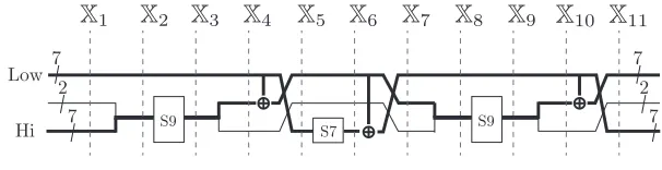
S9

S7

7 2

7

7 2

7 Hi

Low

S9

Fig. 4.Structure ofF Ifunction

5.1 Division Property for F I function

We evaluate the propagation characteristic of the division property for the F I function by using those for MISTY S-boxes shown in Sect. 4.1. Since there are a zero-extended XOR and a truncated XOR in theF I function, we use a new representation, in which the internal state is expressed in two 7-bit values and one 2-bit value. Figure 4 shows the structure of theF I function with our representation, where we remove the XOR of sub keys because it does not affect the division property.

LetX1be the input multiset of theF I function. We define every multisetX2,X3, . . . ,X11

in Fig. 4. Here, elements of the multisetX1,X5,X6, andX11take a value of (F72×F22×F72).

Elements of the multiset X2, X3, X8, and X9 take a value of (F92 ×F72). Elements of the

multisetX4,X7, andX10take a value of (F22×F72×F72). Since elements ofX1 andX11take a

value of (F72×F22×F72), the propagation for theF I function is calculated onD 7,2,7

k(1)_,k(2)_,...,k(q).

Here, the propagation is calculated with the following steps.

From X1 to X2: A 9-bit value is created by concatenating the first 7-bit value with the

second 2-bit value. The propagation characteristic can be evaluated by using Rule 5.

From X2 to X3: The 9-bit S-box S9 is applied to the first 9-bit value. The propagation

characteristic can be evaluated by using Rule 1.

From X3 to X4: The 9-bit output value is split into a 2-bit value and a 7-bit value. The

propagation characteristic can be evaluated by using Rule 4.

From X4 to X5: The second 7-bit value is XORed with the last 7-bit value, and then, the

order is rotated. The propagation characteristic can be evaluated by using Rule 2 and Rule 3.

From X5 to X6: The 7-bit S-box S7 is applied to the first 7-bit value. The propagation

characteristic can be evaluated by using Rule 1.

From X6 to X7: The first 7-bit value is XORed with the last 7-bit value, and then, the

order is rotated. The propagation characteristic can be evaluated by using Rule 2 and Rule 3.

From X7 to X8: A 9-bit value is created by concatenating the first 2-bit value with the

second 7-bit value. The propagation characteristic can be evaluated by using Rule 5.

From X8 to X11: The propagation characteristic is the same as that fromX2 toX5.

As an example, we show the propagation characteristic when X1 has the division property

D7_[4,2_,2,_,7_6] in Appendix E. Algorithm 1 creates the propagation characteristic table for the F I

function. It calls SizeReduce, where redundant elements are eliminated, i.e., it eliminates k(i) if there exists j satisfying k(i) k(j). Algorithm 1 only creates the propagation char-acteristic table for which the input property is represented by D7_k,2,7. If any input multiset

2

Algorithm 1 Propagation forF I function

1: procedureFIEval(k1, k2, k3)

2: k(1)_,k(2)_{, . . . ,k}(q)_⇐

S9Eval(k) ._X1→X5

3: k(1),k(2), . . . ,k(q)⇐S7Eval(k(1),k(2), . . . ,k(q)) .X5→X7

4: k(1)_,k(2)_{, . . . ,k}(q)_⇐S9Eval(k(1)_,k(2)_{, . . . ,k}(q)_{) .}

X7→X11 5: returnSizeReduce(k(1),k(2), . . . ,k(q))

6: end procedure

1: procedureS9Eval(k(1), . . . ,k(q)) 2: q0⇐0

3: fori⇐1 toqdo

4: (`, c, r)⇐(k1(i), k (i) 2 , k

(i) 3 )

5: k⇐`+c

6: if k <9then

7: k⇐ dk/2e

8: end if

9: forc0⇐0 to min(2, k)do

10: forx⇐0 tordo

11: `0⇐r−x

12: r0⇐k−c0+x

13: if r0≤7then

14: q0⇐q0+ 1

15: k0(q0)⇐(`0, c0, r0)

16: end if

17: end for

18: end for

19: end for

20: returnk0(1),k0(2), . . . ,k0(q0)

21: end procedure

22: procedureS7Eval(k(1), . . . ,k(q)) 23: q0⇐0

24: fori⇐1 toq do

25: (`, c, r)⇐(k(1i),k (i) 2 ,k

(i) 3 )

26: k⇐`

27: if k= 6then

28: k⇐4

29: else if k <6then

30: k⇐ dk/3e

31: end if

32: forx⇐0 tordo

33: `0⇐c

34: c0⇐r−x

35: r0⇐k+x

36: if r0≤7then

37: q0⇐q0+ 1

38: k0(q0)⇐(`0, c0, r0)

39: end if

40: end for

41: end for

42: returnk0(1)_,k0(2)_{, . . . ,k}0(q0)

43: end procedure

FI FI FI

Fig. 5.Structure ofF Ofunction

is evaluated, we need to know the propagation characteristic of D7,2,7

k(1)_,k(2)_,...,k(q). However,

we do not evaluate such propagation in advance because it can easily be evaluated by the table for which the input property is represented by D7_k,2,7. We show all propagation char-acteristic tables in Appendix G. Moreover, we experimentally search for the propagation characteristic (see Appendix F).

5.2 Division Property for F O function

We next evaluate the propagation characteristic of the division property for theF Ofunction by using the propagation characteristic table of theF Ifunction. Figure 5 shows the structure of the F O function, where we remove the XOR of sub keys because it does not affect the division property. The input and output of theF Ofunction take the value of (F72×F22×F72×

F72×F22×F72). Therefore, the propagation for theF Ofunction is calculated onD

7,2,7,7,2,7

Algorithm 2 Propagation forF O function

1: procedureFOEval(k1, k2, k3, k4, k5, k6) 2: k(1)_,k(2)_{, . . . ,k}(q)_⇐

FORound(k)

3: k(1),k(2), . . . ,k(q)⇐FORound(k(1),k(2), . . . ,k(q)) 4: k(1)_,k(2)_{, . . . ,k}(q)_⇐FORound(k(1)_,k(2)_{, . . . ,k}(q)₎ 5: returnSizeReduce(k(1),k(2), . . . ,k(q))

6: end procedure

1: procedureFORound(k(1)_,k(2)_{, . . . ,k}(q)₎ 2: q0⇐0

3: fori= 1 toqdo

4: y(1),y(2), . . . ,y(qy)_⇐FIEval(k(i) 1 , k

(i) 2 , k

(i) 3 ) 5: forj= 1 toqy do

6: for allxs.t. (x1≤k4(i))∧(x2≤k(5i))∧(x3≤k(6i))do 7: k0⇐(k(₄i)−x1, k

(i) 5 −x2, k

(i) 6 −x3, y

(j) 1 +x1, y

(j) 2 +x2, y

(j) 3 +x3) 8: if (k40 ≤7)∧(k

0

5≤2)∧(k

0

6≤7)then

9: q0⇐q0+ 1

10: k0(q0)_⇐k0

11: end if

12: end for

13: end for

14: end for

15: returnk0(1),k0(2), . . . ,k0(q0)

16: end procedure

Similar to that for the F I function, we create the propagation characteristic table for the F O function (see Algorithm 2). We create only a table for which the input property is represented by D_k7,2,7,7,2,7 and the output property is represented by D7,2,7,7,2,7

k(1)_,k(2)_,...,k(q). As an

example, the propagation characteristic table fromD7_[1,2_,1,_,7₂,_,7₃,_,2₁,7_,5] is shown in Appendix H.

5.3 Division Property for FL Layer

MISTY1 has the FL layer, which consists of twoF Lfunctions and is applied once every two rounds. In the F L function, the right half of the input is XORed with the AND between the left half and a sub key KLi,1. Then, the left half of the input is XORed with the OR

between the right half and a sub keyKLi,2.

Since the input and the output of the F L function take the value of F72 ×F22×F72×

F72×F22×F72, the propagation for the F Lfunction is calculated on D

7,2,7,7,2,7

k(1)_,k(2)_,...,k(q).FlEval

in Algorithm 3 calculates the propagation characteristic table for the F L function, where SizeReduce eliminates k(i) if there exists j satisfying k(i) k(j). Moreover, the FL layer consists of twoF Lfunctions. Therefore, we have to consider the propagation characteristic of the division propertyD_k7,2,7,7,2,7,7,2,7,7,2,7, where eachF Lfunction is applied to the left half and the right one.FlLayerEvalin Algorithm 3 calculates the propagation characteristic of the division property for the FL layer.

5.4 Path Search for Integral Characteristic on MISTY1

We created the propagation characteristic table for the F I and F O functions in Sect. 5.1 and 5.2, respectively. Moreover, we showed the propagation characteristic for the FL layer in Sect. 5.3. By assembling these propagation characteristics, we create an algorithm to search for integral characteristics on MISTY1. Since the input and the output are represented as eight 7-bit values and four 2-bit values, the propagation is calculated onD7,2,7,7,2,7,7,2,7,7,2,7

Algorithm 3 Propagation for FL layer

1: procedureFlEval(k1, k2, . . . , k6) 2: q0⇐0

3: (`, c, r)⇐(k1+k4, k2+k5, k3+k6) 4: fork10 ⇐0 to min(7, `)do

5: fork20 ⇐0 to min(2, c)do 6: fork03⇐0 to min(7, r)do

7: (k04, k05, k6)0 ⇐(`−k10, c−k02, r−k03) 8: if (k40 ≤7)∧(k

0

5≤2)∧(k

0

6≤7) then

9: q0⇐q0+ 1

10: k0(q0)⇐(k01, k02, k30, k04, k50, k06)

11: end if

12: end for

13: end for

14: end for

15: returnSizeReduce(k(1)_,k(2)_{, . . . ,k}(q0)₎

16: end procedure

1: procedureFlLayerEval(k(1),k(2), . . . ,k(q)) 2: q0⇐0

3: fori⇐1 toqdo

4: `(1)<sub>,`</sub>(2)<sub>, . . . ,`</sub>(q`)_⇐FlEval(k(i) 1 , k

(i) 2 , . . . , k

(i) 6 ) 5: r(1),r(2), . . . ,r(qr)_⇐FlEval(k(i)

7 , k (i) 8 , . . . , k

(i) 12) 6: forj⇐1 toq`do

7: forj0⇐1 toqr do

8: q0⇐q0+ 1

9: k0(q0)⇐(`(1j), ` (j) 2 , `

(j) 3 , `

(j) 4 , `

(j) 5 , `

(j) 6 , r

(j0) 1 , r

(j0) 2 , r

(j0) 3 , r

(j0) 4 , r

(j0) 5 , r

(j0) 6 )

10: end for

11: end for

12: end for

13: return (k0(1),k0(2), . . . ,k0(q0))

14: end procedure

The FL layer is first applied to plaintexts, and it deteriorates the propagation of the division property. Therefore, we first remove only the first FL layer and search for integral characteristics on MISTY1 without the first FL layer. The method for passing through the first FL layer is shown in the next paragraph. Algorithm 4 shows the search algorithm for in-tegral characteristics on MISTY1 without the first FL layer. The straightforward implemen-tation requires impractical calculation time because the perfect processing of SizeReduce requiresO(q02_{) time complexity. Notice that the result of Algorithm 4 does not change even}

if we do not perform SizeReduce. Therefore, we roughly but fast perform SizeReduce. Since the excessive rough SizeReduce causes redundant processing in the next round, we have to search for efficient degree of roughness.

As a result, we can construct 6-round integral characteristics without the first and last

F L layers. Each characteristic uses 263 _{chosen plaintexts, where any one bit of the first}

Algorithm 4 Path search forr-round characteristics without first FL layer

1: procedureRoundFuncEval(k(1)_,k(2)_{, . . . ,k}(q)₎ 2: q0= 0

3: fori⇐1 toqdo

4: for allxs.t.xj≤kj(i)for allj= 1,2, . . . ,6do

5: (r1, r2, r3)⇐(k (i) 1 −x1, k

(i) 2 −x2, k

(i) 3 −x3) 6: (r4, r5, r6)⇐(k4(i)−x4, k5(i)−x5, k6(i)−x6) 7: y(1),y(2), . . . ,y(qy)_⇐FOEval(x

1, x2, x3, x4, x5, x6)

8: fori0⇐1 toqydo

9: (`1, `2, `3)⇐(k (i) 7 +y

(i0) 1 , k

(i) 8 +y

(i0) 2 , k

(i) 9 +y

(i0) 3 ) 10: (`4, `5, `6)⇐(k10(i)+y

(i0) 4 , k

(i) 11 +y

(i0) 5 , k

(i) 12 +y

(i0) 6 )

11: if `j0≤7 forj0∈ {1,3,4,6}and`_j0 ≤2 forj0∈ {2,5}then

12: q0⇐q0+ 1

13: k0(q0)⇐(`1, `2, `3, `4, `5, `6, r1, r2, r3, r4, r5, r6)

14: end if

15: end for

16: end for

17: end for

18: returnSizeReduce(k0(1)_,k0(2)_{, . . . ,k}0(q0)₎

19: end procedure

1: procedureMisty1Eval(k1, k2, . . . , k12, r)

2: k(1)_,k(2)_{, . . . ,k}(q)_{⇐RoundFuncEval(k) .1st round}

3: fori= 1 tordo

4: if iis eventhen

5: k(1),k(2), . . . ,k(q)⇐FlLayerEval(k(1),k(2), . . . ,k(q)) .FL Layer

6: end if

7: k(1),k(2), . . . ,k(q)⇐RoundFuncEval(k(1),k(2), . . . ,k(q)) .(i+1)th round

8: end for

9: end procedure

As shown in Sect. 4, the S7 of MISTY1 has the vulnerable property thatD47 is provided

from D7

6. Interestingly, assuming that S7 does not have this property (change lines 27–31

inS7Eval), our algorithm cannot construct the 6-round characteristic.

We already know that MISTY1 has the 14th order differential characteristic, which is shown in [THK99], and the principle was also discussed in [BF00,CV02]. We also evaluate the principle of the characteristic by using the propagation characteristic of the division property. As a result, we confirm that the characteristic always exists if each algebraic degree S9 and S7 is 2 and 3, respectively. This result implies that the existence of the 14th

order differential characteristic is only derived from the algebraic degree of S-boxes. Namely, even if different S-boxes are chosen in S7 and S9, the 14th order differential characteristic

exists unless the algebraic degree increases. The detail is discussed in Appendix D.

Passage of First FL Layer Our new characteristic removes the first FL layer. Therefore, we have to create a set of chosen plaintexts to construct integral characteristics by using guessed round keys KL1,1 and KL1,2. Here, we have to carefully choose the set of chosen

plaintexts to avoid the use of the full code book (see Fig. 7, Fig. 8, and Fig. 9). In every figure,Aidenotes for which we prepare an input set thatibits are active. As an example, we consider an integral characteristic for which the first one bit is constant and the remaining 63 bits are active. Since all bits of the right half are active, we focus only on the left half. We first guess that KL1,2[1] = 1, and we then prepare the set of plaintexts like in

FO

FO

FO

FO

FL FL

FO

FO

FL FL

Fig. 6.New 6-round integral characteristic

KL1,1

KL1,2

(0A15 0A15) (0A15 1A15)

(1A15 A16) KL1,2[1]=1

KL1,1[1]=*

Fig. 7.KL1,2= 1

KL1,1

KL1,2

(0A15 1A15) (1A15 0A15)

(1A15 A16) KL1,2[1]=0

KL1,1[1]=0

Fig. 8.KL1,1= 0, KL1,2= 0

KL1,1

KL1,2

(0A15 0A15) (1A15 0A15)

(0A15 A16) KL1,2[1]=0

KL1,1[1]=1

Fig. 9.KL1,1= 1, KL1,2= 0

plaintexts like in Fig. 8. Moreover, we guess that (KL1,1[1], KL1,2[1]) = (1,0), and we then

prepare the set of plaintexts like in Fig. 9. Their chosen plaintexts construct 6-round integral characteristics if the guessed key bits are correct. Notice that we do not use 262 _chosen

plaintexts as (1A15 1A15 A16 A16). Thus, our integral characteristics use 264−262≈263.58

chosen plaintexts.

6 Key Recovery Using New Integral Characteristic

This section shows the key recovery step of our cryptanalysis, which uses the 6-round integral characteristic shown in Sect. 5. In the characteristic, the left 7-bit value of XL

7 is

balanced. To evaluate this balanced seven bits, we have to calculate two FL layers and one

F O function by using the guessed round keys. Figure 10 shows the structure of our key recovery step.

6.1 Sub Key Recovery Using Partial-Sum Technique

We guessKL1,1[i](=K1[i]) andKL1,2[i](=K70[i]) and then prepare a set of chosen plaintexts

to construct an integral characteristic. In the characteristic, seven bits XL

7[1, . . . ,7] are

balanced. Therefore, we evaluate whether or not XL

7[j] is balanced for j∈ {1,2, . . . ,7} by

using a partial-sum technique [FKL+_00].

BUU UUU

C L[1-16] _C L_{[17-32] C} R_{[j] C} R_[16+j]

Fig. 10.Key recovery step

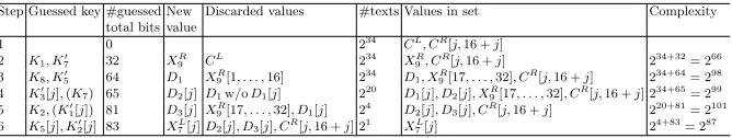
Table 2.Procedure of key recovery step

Step Guessed key #guessed New Discarded values #texts Values in set Complexity

total bits value

1 0 234

CL

, CR

[j,16 +j]

2 K1, K07 32 X

R

9 C

L

234

XR

9, C

R

[j,16 +j] 234+32

= 266

3 K8, K05 64 D1 XR9[1, . . . ,16] 234 D1, X9R[17, . . . ,32], CR[j,16 +j] 234+64= 298

4 K03[j],(K7) 65 D2[j]D1w/oD1[j] 220 D1[j], D2[j], X9R[17, . . . ,32], CR[j,16 +j] 234+65= 299

5 K2,(K10[j]) 81 D3[j]XR9[17, . . . ,32], D1[j] 24 D2[j], D3[j], CR[j,16 +j] 220+81= 2101

6 K5[j], K20[j] 83 X L

7[j]D2[j], D3[j], CR[j,16 +j] 21 X7L[j] 2

4+83

= 287

and calculate the XOR ofXL

7[j]. Table 2 summarizes the procedure of the key recovery step,

where every value is defined in Fig. 10.

Step 1 Prepare the memory that stores how many times each 34-bit value (CL_{, C}R_[j,16+j]) appears, and pick the values that appear odd times.

Step 2 Guess 32-bit (K1, K70), and calculate X9R from CL. Delete CL from the memory,

and storeXR

9 into the memory. Namely, there are 34-bit value (X9R, CR[j,16 +j]) in the

memory. The time complexity of Step 2 is 234_×232_{= 2}66_.

Step 3 Guess 32-bit (K8, K50), and calculate D1 from X9R. Delete X9R[1, . . . ,16] from the

memory, and storeD1into the memory. Namely, there are 34-bit value (D1, X9R[17, . . . ,32], CR[j,16+

j]) in the memory. The time complexity of Step 3 is 234_×264_{= 2}98_.

Step 4 Guess 1-bit K₃0[j], get K7 from (K70, K8), which is already guessed in Step 2 and

Step 3, and calculateD2[j] fromD1. DeleteD1withoutD1[j] from the memory, and store

D2[j] into the memory. Namely, there are 20-bit value (D1[j], D2[j], X9R[17, . . . ,32], CR[j,16+

j]) in the memory. The time complexity of Step 4 is 234_×265_{= 2}99_.

Step 5 Guess 32-bit K2, get K10[j] from (K1, K2), which is already guessed in Step 2 and

Step 5, and calculate D3[j] from (X9R[17, . . . ,32], D1[j]). Delete (X9R[17, . . . ,32], D1[j])

(D2[j], D3[j], CR[j,16 +j]) in the memory. The time complexity of Step 5 is 220×281=

2101_.

Step 6 Guess 2-bit (K5[j], K20[j]), getK30[j], which is already guessed in Step 4, and

calcu-late XL

7[j] from (D2[j], D3[j], CR[j,16 +j]). The time complexity of Step 6 is 24×283=

287_.

The total time complexity is

266_{+ 2}98_{+ 2}99_{+ 2}101_{+ 2}87_≈2101.5_.

We repeat the above six steps for j ∈ {1,2, . . . ,7}. Therefore, the time complexity of the key recovery step is 7×2101.5 _{= 2}104.3_.

The key recovery step has to guess the 124-bit key

K1, K2, K5[1, . . . ,7], K7, K8,

K₁0[1, . . . ,7], K₂0[1, . . . ,7], K₃0[1, . . . ,7], K₅0, K₇0.

Here,K₇0 and K₁0[1, . . . ,7] are uniquely determined by guessingK7, K8 andK1, K2,

respec-tively. Thus, the guessed key bit size is reduced to

K1, K2, K5[1, . . . ,7], K7, K8,

K₂0[1, . . . ,7], K₃0[1, . . . ,7], K₅0,

and it becomes 101 bits. Moreover, since we already guessed 2 bits, i.e.,K1[i] andK70[i], to

construct integral characteristics, the guessed key bit size is reduced to 99 bits. For wrong keys, the probability that XL

7[1, . . . ,7] is balanced is 2−7. Therefore, the number of the

candidates of round keys is reduced to 292_{. Finally, we guess the 27 bits:}

K5[8, . . . ,16], K20[8, . . . ,16], K30[8, . . . ,16].

Notice thatK3,K4, andK6are uniquely determined from (K2, K20), (K3, K30), and (K5, K50),

respectively. Therefore, the total time complexity is 292+27 _{= 2}119_{. We guess the correct key}

from 2119 _{candidates by using two plaintext-ciphertext pairs, and the time complexity is}

2119 _{+ 2}119−64 _{≈ 2}119_{. We have to execute the above procedure against (K}

1[i], K70[i]) =

(0,0),(0,1),(1,0),(1,1), and the time complexity becomes 4×2119 _{= 2}121_.

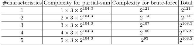
6.2 Trade-off between Time and Data Complexity

In Sect. 6.1, we use only one set of chosen plaintexts, where (264₋₂62_{) chosen plaintexts are}

required. Since the probability that wrong keys are not discarded is 2−7_{, a brute-force search}

is required with a time complexity of 2128−7_{= 2}119_{, and it is larger than the time complexity}

of the partial-sum technique. Therefore, if we have a higher number of characteristics, the total time complexity can be reduced.

To prepare several characteristics, we choose some constant bits from seven bits (i ∈ {1,2, . . . ,7}). If we use a characteristic with i = 1, we use chosen plaintexts for which plaintextPL _{takes the following values}

(00A14 00A14),(00A14 01A14),(01A14 00A14),(01A14 01A14),

(00A14 10A14),(00A14 11A14),(01A14 10A14),(01A14 11A14),

Table 3.Trade-off between time and data complexity

#characteristics Complexity for partial-sum Complexity for brute-force Total

1 1×3×2104.3 ₂121 ₂121

2 2×3×2104.3 2114 2114

3 3×3×2104.3 2107 2108.3

4 4×3×2104.3 ₂100 ₂107.9

5 5×3×2104.3 ₂93 ₂108.2

whereA14 denotes that all values appear the same number independent of other bits, e.g.,

(00A14 00A14) uses 260chosen plaintexts because PRalso takes all values. Moreover, if we

use a characteristic with i= 2, we use chosen plaintexts for which PL _{takes the following} values

(00A14 00A14),(00A14 10A14),(10A14 00A14),(10A14 10A14),

(00A14 01A14),(00A14 11A14),(10A14 01A14),(10A14 11A14),

(01A14 00A14),(01A14 10A14),(11A14 00A14),(11A14 10A14).

When both characteristics are used, they do not require choosing plaintexts for which PL takes (11A14 11A14). Therefore, (264−260) chosen plaintexts are required, and the

proba-bility that wrong keys are not discarded becomes 2−14_{. Similarly, when three characteristics,}

which require (264₋₂58_{) chosen plaintexts, are used, the probability that wrong keys are}

not discarded becomes 2−21_.

Table 3 summarizes the trade-off between time and data complexity. For the use of each characteristic, we have to execute three key recoveries with the partial-sum technique, i.e., for (KL1,1[1], KL1,2[1])∈ {(∗,1),(0,0),(1,0)}. It shows that the use of four characteristics

is optimized from the perspective of time complexity. Namely, when (264₋₂56_{) ≈ 2}63.994

chosen plaintexts are required, the time complexity to recovery the secret key is 2107.9_.

7 Conclusions

In this paper, we showed a cryptanalysis of the full MISTY1. MISTY1 was well evaluated and standardized by several projects, such as CRYPTREC, ISO/IEC, and NESSIE. We constructed a new integral characteristic by using the propagation characteristic of the division property. Here, we improved the division property by optimizing a public S-box. As a result, a new 6-round integral characteristic is constructed, and we can recover the secret key of the full MISTY1 with 263.58 _{chosen plaintexts and 2}121 _{time complexity. If}

we can use 263.994 _{chosen plaintexts, our attack can recover the secret key with a time}

complexity of 2107.9_.

References

Bar15. Achiya Bar-On. Improved higher-order differential attacks on MISTY1. InFSE, 2015.

BC13. Christina Boura and Anne Canteaut. On the influence of the algebraic degree of f-1 on the algebraic degree of G◦F. IEEE Transactions on Information Theory, 59(1):691–702, 2013.

BF00. Steve Babbage and Laurent Frisch. On MISTY1 higher order differential cryptanalysis. In Dongho Won, editor,ICISC, volume 2015 ofLNCS, pages 22–36. Springer, 2000.

CRY13. CRYPTREC. Specifications of e-government recommended ciphers. available at http://www. cryptrec.go.jp/english/method.html, 2013.

CV02. Anne Canteaut and Marion Videau. Degree of composition of highly nonlinear functions and applications to higher order differential cryptanalysis. In Lars R. Knudsen, editor,EUROCRYPT, volume 2332 ofLNCS, pages 518–533. Springer, 2002.

DK08. Orr Dunkelman and Nathan Keller. An improved impossible differential attack on MISTY1. In Josef Pieprzyk, editor,ASIACRYPT, volume 5350 ofLNCS, pages 441–454. Springer, 2008. DKR97. Joan Daemen, Lars R. Knudsen, and Vincent Rijmen. The block cipher Square. In Eli Biham,

editor,FSE, volume 1267 ofLNCS, pages 149–165. Springer, 1997.

FKL+00. Niels Ferguson, John Kelsey, Stefan Lucks, Bruce Schneier, Michael Stay, David Wagner, and Doug Whiting. Improved cryptanalysis of Rijndael. In Bruce Schneier, editor,FSE, volume 1978 ofLNCS, pages 213–230. Springer, 2000.

HTK04. Yasuo Hatano, Hidema Tanaka, and Toshinobu Kaneko. Optimization for the algebraic method and its application to an attack of MISTY1. IEICE Transactions, 87-A(1):18–27, 2004.

ISO05. ISO/IEC. JTC1: ISO/IEC 18033: Security techniques – encryption algorithms – part 3: Block ciphers, 2005.

Knu94. Lars R. Knudsen. Truncated and higher order differentials. In Bart Preneel, editor,FSE, volume 1008 ofLNCS, pages 196–211. Springer, 1994.

KW02. Lars R. Knudsen and David Wagner. Integral cryptanalysis. In Joan Daemen and Vincent Rijmen, editors,FSE, volume 2365 ofLNCS, pages 112–127. Springer, 2002.

Lai94. Xuejia Lai. Higher order derivatives and differential cryptanalysis. InCommunications and

Cryp-tography, volume 276 of The Springer International Series in Engineering and Computer Science,

pages 227–233, 1994.

Mat93. Mitsuru Matsui. Linear cryptanalysis method for DES cipher. In Tor Helleseth, editor,

EURO-CRYPT, volume 765 ofLNCS, pages 386–397. Springer, 1993.

Mat96. Mitsuru Matsui. New structure of block ciphers with provable security against differential and linear cryptanalysis. In Dieter Gollmann, editor,FSE, volume 1039 ofLNCS, pages 205–218. Springer, 1996.

Mat97. Mitsuru Matsui. New block encryption algorithm MISTY. In Eli Biham, editor,FSE, volume 1267 ofLNCS, pages 54–68. Springer, 1997.

NES04. NESSIE. New european schemes for signatures, integrity, and encryption. available at https: //www.cosic.esat.kuleuven.be/nessie/, 2004.

NK95. Kaisa Nyberg and Lars R. Knudsen. Provable security against a differential attack. J. Cryptology, 8(1):27–37, 1995.

Nyb94. Kaisa Nyberg. Linear approximation of block ciphers. In Alfredo De Santis, editor,EUROCRYPT, volume 950 ofLNCS, pages 439–444. Springer, 1994.

OM00. Hidenori Ohta and Mitsuru Matsui. A description of the MISTY1 encryption algorithm. available athttps://tools.ietf.org/html/rfc2994, 2000.

SHZ+15. Bing Sun, Xin Hai, Wenyu Zhang, Lei Cheng, and Zhichao Yang. New observation on division property. IACR Cryptology ePrint Archive, 2015:459, 2015.

THK99. Hidema Tanaka, Kazuyuki Hisamatsu, and Toshinobu Kaneko. Strenght of MISTY1 without FL function for higher order differential attack. In Marc P. C. Fossorier, Hideki Imai, Shu Lin, and Alain Poli, editors,AAECC-13, volume 1719 of LNCS, pages 221–230. Springer, 1999.

Tod15. Yosuke Todo. Structural evaluation by generalized integral property. In Elisabeth Oswald and Marc Fischlin, editors,EUROCRYPT Part I, volume 9056 ofLNCS, pages 287–314. Springer, 2015. TSSK08. Yukiyasu Tsunoo, Teruo Saito, Maki Shigeri, and Takeshi Kawabata. Higher order differential

A MISTY S-boxes

The ANF ofS7 is represented as

y[0] =x[0]⊕x[1]x[3]⊕x[0]x[3]x[4]⊕x[1]x[5]⊕x[0]x[2]x[5]⊕x[4]x[5] ⊕x[0]x[1]x[6]⊕x[2]x[6]⊕x[0]x[5]x[6]⊕x[3]x[5]x[6]⊕1,

y[1] =x[0]x[2]⊕x[0]x[4]⊕x[3]x[4]⊕x[1]x[5]⊕x[2]x[4]x[5]⊕x[6]⊕x[0]x[6] ⊕x[3]x[6]⊕x[2]x[3]x[6]⊕x[1]x[4]x[6]⊕x[0]x[5]x[6]⊕1,

y[2] =x[1]x[2]⊕x[0]x[2]x[3]⊕x[4]⊕x[1]x[4]⊕x[0]x[1]x[4]⊕x[0]x[5]⊕x[0]x[4]x[5] ⊕x[3]x[4]x[5]⊕x[1]x[6]⊕x[3]x[6]⊕x[0]x[3]x[6]⊕x[4]x[6]⊕x[2]x[4]x[6], y[3] =x[0]⊕x[1]⊕x[0]x[1]x[2]⊕x[0]x[3]⊕x[2]x[4]⊕x[1]x[4]x[5]⊕x[2]x[6]

⊕x[1]x[3]x[6]⊕x[0]x[4]x[6]⊕x[5]x[6]⊕1,

y[4] =x[2]x[3]⊕x[0]x[4]⊕x[1]x[3]x[4]⊕x[5]⊕x[2]x[5]⊕x[1]x[2]x[5]⊕x[0]x[3]x[5] ⊕x[1]x[6]⊕x[1]x[5]x[6]⊕x[4]x[5]x[6]⊕1,

y[5] =x[0]⊕x[1]⊕x[2]⊕x[0]x[1]x[2]⊕x[0]x[3]⊕x[1]x[2]x[3]⊕x[1]x[4] ⊕x[0]x[2]x[4]⊕x[0]x[5]⊕x[0]x[1]x[5]⊕x[3]x[5]⊕x[0]x[6]⊕x[2]x[5]x[6], y[6] =x[0]x[1]⊕x[3]⊕x[0]x[3]⊕x[2]x[3]x[4]⊕x[0]x[5]⊕x[2]x[5]⊕x[3]x[5]

⊕x[1]x[3]x[5]⊕x[1]x[6]⊕x[1]x[2]x[6]⊕x[0]x[3]x[6]⊕x[4]x[6]⊕x[2]x[5]x[6].

Moreover, the ANF of S9 is represented as

y[0] =x[0]x[4]⊕x[0]x[5]⊕x[1]x[5]⊕x[1]x[6]⊕x[2]x[6]⊕x[2]x[7]⊕x[3]x[7]⊕x[3]x[8] ⊕x[4]x[8]⊕1,

y[1] =x[0]x[2]⊕x[3]⊕x[1]x[3]⊕x[2]x[3]⊕x[3]x[4]⊕x[4]x[5]⊕x[0]x[6]⊕x[2]x[6] ⊕x[7]⊕x[0]x[8]⊕x[3]x[8]⊕x[5]x[8]⊕1,

y[2] =x[0]x[1]⊕x[1]x[3]⊕x[4]⊕x[0]x[4]⊕x[2]x[4]⊕x[3]x[4]⊕x[4]x[5]⊕x[0]x[6] ⊕x[5]x[6]⊕x[1]x[7]⊕x[3]x[7]⊕x[8],

y[3] =x[0]⊕x[1]x[2]⊕x[2]x[4]⊕x[5]⊕x[1]x[5]⊕x[3]x[5]⊕x[4]x[5]⊕x[5]x[6] ⊕x[1]x[7]⊕x[6]x[7]⊕x[2]x[8]⊕x[4]x[8],

y[4] =x[1]⊕x[0]x[3]⊕x[2]x[3]⊕x[0]x[5]⊕x[3]x[5]⊕x[6]⊕x[2]x[6]⊕x[4]x[6] ⊕x[5]x[6]⊕x[6]x[7]⊕x[2]x[8]⊕x[7]x[8],

y[5] =x[2]⊕x[0]x[3]⊕x[1]x[4]⊕x[3]x[4]⊕x[1]x[6]⊕x[4]x[6]⊕x[7]⊕x[3]x[7] ⊕x[5]x[7]⊕x[6]x[7]⊕x[0]x[8]⊕x[7]x[8],

y[6] =x[0]x[1]⊕x[3]⊕x[1]x[4]⊕x[2]x[5]⊕x[4]x[5]⊕x[2]x[7]⊕x[5]x[7]⊕x[8] ⊕x[0]x[8]⊕x[4]x[8]⊕x[6]x[8]⊕x[7]x[8]⊕1,

y[7] =x[1]⊕x[0]x[1]⊕x[1]x[2]⊕x[2]x[3]⊕x[0]x[4]⊕x[5]⊕x[1]x[6]⊕x[3]x[6] ⊕x[0]x[7]⊕x[4]x[7]⊕x[6]x[7]⊕x[1]x[8]⊕1,

B Proof of Propagation Rules

B.1 Proof of Rule 1 (Substitution)

LetF be a function that consists ofm S-boxes, whereFi denotes theith S-box and the bit length and the algebraic degree is ni bits and di, respectively. The input and the output take a value of (Fn21 ×F

n2

2 × · · · ×F

nm

2 ), and X and Y denote the input multiset and the

output multiset, respectively.

Assuming that the multisetXhas the division propertyD_kn1(1),n_,2_k,...,n(2)_,...,m_k(q),

L

x∈Xπu(x) = 0

ifW(u)k(i) holds for all i(1≤i≤q). First, we only apply the first S-box and evaluate

the division property of the multiset whose elements are represented by (F1(x1), x2, . . . , xm). The division property is evaluated as follows

M

x∈X

πv(F1(x1), x2, . . . , xm) =

M

x∈X

(πv1◦F1)(xi)× m

Y

i=2

πvi(xi)

!

=M

x∈X



 M

u1∈Fn21

a(πv1◦F1)

u1 πu1(x1)



×

m

Y

i=2

πvi(xi)

!

= M

u1∈Fn21

M

x∈_X

a(πv1◦F1)

u1 πu1(x1)× m

Y

i=2

πvi(xi)

!!

.

Therefore, for any v∈(Fn21×F

n2

2 × · · · ×Fn2m), the parity becomes 0 if

M

x∈X

a(πv₁◦F1)

u1 πu1(x1)× m

Y

i=2

πvi(xi)

!

=a(πv₁◦F1) u1

M

x∈X

π_{(u1,v2,v3,...,vm)}(x)

is 0 for allu1 ∈Fn21. Since the algebraic degree of (πv1◦F1) is at mostw(v1)×d,a

(πv1◦F1)

u1 = 0

ifw(u1)> w(v1)×d1. Therefore, the parity becomes unknown only if we cannot determine

the value of L

x∈Xπ(u1,v2,v3,...,vm)(x) forw(u1)≤w(v1)×d1. From the division property of

the input multiset,L

x∈_Xπ(u1,v2,v3,...,vm)(x) = 0 if W(v1, u2, u3, . . . , um)k

(i) _{holds for all}

i(1≤i≤q). Therefore, the following relation

W(u1, v2, v3, . . . , vm)k(i)⇒(w(v1)×d1, w(v2), . . . , w(vm))k(i)

⇒(w(v1), w(v2), . . . , w(vm))

&

k(₁i) d1

'

, k(₂i), k₃(i), . . . , , k(_mi)

!

holds, and then the division property of the output multiset becomesDn1,n2,...,nm

k0(1)_,k0(2)_,...,k0(q), where

(k₁0(j), k₂0(j), . . . , k0(j)

m ) =

&

k(_ij) di

'

, k0₂(j), . . . , k0(j)

m

!

for 1≤j≤q.

B.2 Proof of Rule 2 (Copy)

LetF be a copy function, where the inputxtakes a value ofFn2 and the output is calculated

as (y1, y2) = (x, x). LetXandYbe the input multiset and the output multiset, respectively.

Assuming that the multisetXhas the division propertyD_kn,Lx∈Xπu(x) = 0 forw(u)< k. The division property of Yis evaluated as follows

M

x∈X

π(v1,v2)(x, x) =

M

x∈X

(πv1(x)×πv2(x)).

When w(v1) +w(v2) is less thankat least, the parity is always 0 because Lx∈Xπu(x) = 0

forw(u)< k. Therefore, the division property ofYis D_kn,n0(1)_,k0(2)_,...,k0(k+1) as

k0(i+1)= (k−i, i) for 0≤i≤k.

Thus, Rule 2 is proven.

B.3 Proof of Rule 3 (Compression by XOR)

Let F be a compression function by an XOR, where the input (x1, x2) takes a value of

(Fn2 ×Fn2) and the output is calculated asy =x1⊕x2. LetX and Ybe the input multiset

and the output multiset, respectively.

Assuming that the multisetXhas the division propertyDn,n_k(1)_,k(2)_,...,k(q),

L

x∈_Xπu(x) = 0

ifW(u)k(i) holds for all i(1≤i≤q). The division property ofYis evaluated as follows

M

(x1,x2)∈X

πv(x1⊕x2) =

M

(x1,x2)∈X

πv(x1⊕x2)

= M

(x1,x2)∈X n

Y

i=1

(x1[i]⊕x2[i])v[i]

!

= M

(x1,x2)∈X



 M

w∈{1,2}n

n

Y

i=1

xwi[i]

v[i]

! .

Therefore, for any v∈_Fn

2, the parity becomes 0 if

M

(x1,x2)∈X n

Y

i=1

xwi[i]

v[i]

!

is 0 for allw∈ {1,2}n_{. In this case, the parity becomes unknown only if we choose at least}

k0 bits fromy∈Y, where

k0 = min{k(1)₁ +k(1)₂ , k₁(2)+k₂(2), . . . , k₁(q)+k₂(q)}.

B.4 Proof of Rule 4 (Split)

LetF be a split function, where the inputxtakes a value ofFn2 and the output is calculated

as x = y1ky2, where (y1, y2) takes a value of (Fn21 ×F

n−n1

2 ). Let X and Y be the input

multiset and the output multiset, respectively.

Assuming that the multisetXhas the division propertyDkn,

L

x∈Xπu(x) = 0 forw(u)< k. The division property of Yis evaluated as follows

M

x∈_X

π(v1,v2)(y1, y2) =

M

x∈_X

πv1kv2(y1ky2).

When w(v1) +w(v2) is less thankat least, the parity is always 0 because Lx∈Xπu(x) = 0

forw(u)< k. Therefore, the division property ofYis D_kn01(1),n−_,kn0(2)1 _,...,k0(k+1) as

k0(i+1)= (k−i, i) for 0≤i≤k.

Notice that we cannot choose more than n1 and n−n1 bits from y1 and y2, respectively.

Thus, Rule 4 is proven.

B.5 Proof of Rule 5 (Concatenation)

LetF be a concatenation function, where the input (x1, x2) takes a value of (Fn21×F

n2

2 ) and

the output is calculated as y =x1kx2. Let Xand Ybe the input multiset and the output

multiset, respectively.

Assuming that the multisetXhas the division propertyD_kn(1)1,n_,2_k(2)_,...,k(q),

L

x∈Xπu(x) = 0

ifW(u)k(i) holds for all i(1≤i≤q). The division property ofYis evaluated as follows

M

(x1,x2)∈X

πv(x1kx2) =

M

(x1,x2)∈X

πv1kv2(x1kx2) =

M

(x1,x2)∈X

π(v1,v2)(x1, x2)

Therefore, the parity becomes unknown only if we choose at leastk0 bits fromy∈Y, where

k0 = min{k(1)₁ +k(1)₂ , k₁(2)+k₂(2), . . . , k₁(q)+k₂(q)}.

C Propagation from D_[67,2_,2,_,7₇,_,7₇,2_,2,_,7₇,_,7₇,_,2₂,_,7₇,_,7₇,_,2₂,7_,7]

When the input set has the division propertyD_[67,2_,2,7_,7,_,7₇,_,2₂,_,7₇,_,7₇,_,2₂,_,7₇,_,7₇,2_,2,7_,7], the division property of the set of texts encrypted 6 rounds without the first and the last FL layers is represented asD7,2,7,7,2,7,7,2,7,7,2,7

k(1)_,k(2)_,...,k(132) . Here, 132 vectors are represented as follows:

(0,0,0,0,0,0,0,0,0,0,0,4) (0,0,0,0,0,0,0,0,0,0,1,3) (0,0,0,0,0,0,0,0,0,0,2,2) (0,0,0,0,0,0,0,0,0,1,0,3) (0,0,0,0,0,0,0,0,0,1,1,2) (0,0,0,0,0,0,0,0,0,1,2,1) (0,0,0,0,0,0,0,0,0,2,0,2) (0,0,0,0,0,0,0,0,0,2,1,1) (0,0,0,0,0,0,0,0,0,2,2,0) (0,0,0,0,0,0,0,0,0,3,0,1) (0,0,0,0,0,0,0,0,0,3,1,0) (0,0,0,0,0,0,0,0,0,4,0,0) (0,0,0,0,0,0,0,0,1,0,0,3) (0,0,0,0,0,0,0,0,1,0,1,2) (0,0,0,0,0,0,0,0,1,0,2,1) (0,0,0,0,0,0,0,0,1,1,0,2) (0,0,0,0,0,0,0,0,1,1,1,1) (0,0,0,0,0,0,0,0,1,1,2,0) (0,0,0,0,0,0,0,0,1,2,0,1) (0,0,0,0,0,0,0,0,1,2,1,0) (0,0,0,0,0,0,0,0,1,3,0,0) (0,0,0,0,0,0,0,0,2,0,0,2) (0,0,0,0,0,0,0,0,2,0,1,1) (0,0,0,0,0,0,0,0,2,0,2,0) (0,0,0,0,0,0,0,0,2,1,0,1) (0,0,0,0,0,0,0,0,2,1,1,0) (0,0,0,0,0,0,0,0,2,2,0,0) (0,0,0,0,0,0,0,0,3,0,0,1) (0,0,0,0,0,0,0,0,3,0,1,0) (0,0,0,0,0,0,0,0,4,1,0,0) (0,0,0,0,0,0,0,0,7,0,0,0) (0,0,0,0,0,0,0,1,0,0,0,3) (0,0,0,0,0,0,0,1,0,0,1,2) (0,0,0,0,0,0,0,1,0,0,2,1) (0,0,0,0,0,0,0,1,0,1,0,2) (0,0,0,0,0,0,0,1,0,1,1,1) (0,0,0,0,0,0,0,1,0,1,2,0) (0,0,0,0,0,0,0,1,0,2,0,1) (0,0,0,0,0,0,0,1,0,2,1,0) (0,0,0,0,0,0,0,1,0,3,0,0) (0,0,0,0,0,0,0,1,1,0,0,2) (0,0,0,0,0,0,0,1,1,0,1,1) (0,0,0,0,0,0,0,1,1,0,2,0) (0,0,0,0,0,0,0,1,1,1,0,1) (0,0,0,0,0,0,0,1,1,1,1,0) (0,0,0,0,0,0,0,1,1,2,0,0) (0,0,0,0,0,0,0,1,2,0,0,1) (0,0,0,0,0,0,0,1,2,0,1,0) (0,0,0,0,0,0,0,1,2,1,0,0) (0,0,0,0,0,0,0,1,5,0,0,0) (0,0,0,0,0,0,0,2,0,0,0,2) (0,0,0,0,0,0,0,2,0,0,1,1) (0,0,0,0,0,0,0,2,0,0,2,0) (0,0,0,0,0,0,0,2,0,1,0,1) (0,0,0,0,0,0,0,2,0,1,1,0) (0,0,0,0,0,0,0,2,0,2,0,0) (0,0,0,0,0,0,0,2,1,0,0,1) (0,0,0,0,0,0,0,2,1,0,1,0) (0,0,0,0,0,0,0,2,1,1,0,0) (0,0,0,0,0,0,0,2,4,0,0,0) (0,0,0,0,0,0,1,0,0,0,0,3) (0,0,0,0,0,0,1,0,0,0,1,2) (0,0,0,0,0,0,1,0,0,0,2,1) (0,0,0,0,0,0,1,0,0,1,0,2) (0,0,0,0,0,0,1,0,0,1,1,1) (0,0,0,0,0,0,1,0,0,1,2,0) (0,0,0,0,0,0,1,0,0,2,0,1) (0,0,0,0,0,0,1,0,0,2,1,0) (0,0,0,0,0,0,1,0,0,3,0,0) (0,0,0,0,0,0,1,0,1,0,0,2) (0,0,0,0,0,0,1,0,1,0,1,1) (0,0,0,0,0,0,1,0,1,0,2,0) (0,0,0,0,0,0,1,0,1,1,0,1) (0,0,0,0,0,0,1,0,1,1,1,0) (0,0,0,0,0,0,1,0,1,2,0,0) (0,0,0,0,0,0,1,0,2,0,0,1) (0,0,0,0,0,0,1,0,2,0,1,0) (0,0,0,0,0,0,1,0,2,1,0,0) (0,0,0,0,0,0,1,0,5,0,0,0) (0,0,0,0,0,0,1,1,0,0,0,2) (0,0,0,0,0,0,1,1,0,0,1,1) (0,0,0,0,0,0,1,1,0,0,2,0) (0,0,0,0,0,0,1,1,0,1,0,1) (0,0,0,0,0,0,1,1,0,1,1,0) (0,0,0,0,0,0,1,1,0,2,0,0) (0,0,0,0,0,0,1,1,1,0,0,1) (0,0,0,0,0,0,1,1,1,0,1,0) (0,0,0,0,0,0,1,1,1,1,0,0) (0,0,0,0,0,0,1,1,4,0,0,0) (0,0,0,0,0,0,1,2,0,0,0,1) (0,0,0,0,0,0,1,2,0,0,1,0) (0,0,0,0,0,0,1,2,0,1,0,0) (0,0,0,0,0,0,1,2,3,0,0,0) (0,0,0,0,0,0,2,0,0,0,0,2) (0,0,0,0,0,0,2,0,0,0,1,1) (0,0,0,0,0,0,2,0,0,0,2,0) (0,0,0,0,0,0,2,0,0,1,0,1) (0,0,0,0,0,0,2,0,0,1,1,0) (0,0,0,0,0,0,2,0,0,2,0,0) (0,0,0,0,0,0,2,0,1,0,0,1) (0,0,0,0,0,0,2,0,1,0,1,0) (0,0,0,0,0,0,2,0,1,1,0,0) (0,0,0,0,0,0,2,0,4,0,0,0) (0,0,0,0,0,0,2,1,0,0,0,1) (0,0,0,0,0,0,2,1,0,0,1,0) (0,0,0,0,0,0,2,1,0,1,0,0) (0,0,0,0,0,0,2,1,3,0,0,0) (0,0,0,0,0,0,2,2,2,0,0,0) (0,0,0,0,0,0,3,0,0,0,0,1) (0,0,0,0,0,0,3,0,0,0,1,0) (0,0,0,0,0,0,3,0,0,2,0,0) (0,0,0,0,0,0,3,0,3,0,0,0) (0,0,0,0,0,0,3,1,2,0,0,0) (0,0,0,0,0,0,3,2,1,0,0,0) (0,0,0,0,0,0,4,0,0,1,0,0) (0,0,0,0,0,0,5,0,2,0,0,0) (0,0,0,0,0,0,5,1,1,0,0,0) (0,0,0,0,0,0,5,2,0,0,0,0) (0,0,0,0,0,0,7,0,1,0,0,0) (0,0,0,0,0,0,7,1,0,0,0,0) (0,0,0,0,0,1,0,0,0,0,0,0) (0,0,0,0,1,0,0,0,0,0,0,0) (0,0,0,1,0,0,0,0,0,0,0,0) (0,0,1,0,0,0,0,0,0,0,0,0) (0,1,0,0,0,0,0,0,0,0,0,0) (1,0,0,0,0,0,0,0,0,0,0,1) (1,0,0,0,0,0,0,0,0,0,1,0) (1,0,0,0,0,0,0,0,0,1,0,0) (1,0,0,0,0,0,0,0,1,0,0,0) (1,0,0,0,0,0,0,1,0,0,0,0) (1,0,0,0,0,0,1,0,0,0,0,0) (2,0,0,0,0,0,0,0,0,0,0,0)

Assuming thatXhas the division propertyD_k7,(1)2,7_,k,7(2),2,_,...,7,7_k,2(,7q),7,2,7,

L

x∈_Xxj becomes 0 if there exist k(i) such that k_j(i) is greater than 1. From the last vector of 132 vectors, k1 takes 2.

D 14th Order Differential Characteristic Revisited

In [HTK04] and [TSSK08], they used the 14th order differential characteristic, where 14 bits

PR_{[10−16,26−32] are active and the others are constant. In the characteristic, the first} seven bits of XR

5 are balanced. Moreover, they extended the characteristic to 46th order

differential characteristic, where 14 bitsPL_{[10−16,26−32] and 32 bitsP}R _{are active and} the others are constant. In the characteristic, the first seven bits of XL

5 are balanced. We

revisit their characteristics from the perspective of the propagation characteristic of the division property.

We assume that S9 is a any 9-bit bijective function with degree 2 and S7 is a any 7-bit

bijective function with degree 3. We search for integral characteristics, and then the division property propagates as follows:

D_k7,2,7,7,2,7,7,2,7,7,2,7 4 rounds D7,2,7,7,2,7,7,2,7,7,2,7 k(1)_,k(2)_,...,k(12)

k= (0,0,0,0,0,0,0,0,7,0,0,7) ⇒ k(1) = (1,0,0,0,0,0,0,0,0,0,0,0) k(2) = (0,1,0,0,0,0,0,0,0,0,0,0) k(3) = (0,0,1,0,0,0,0,0,0,0,0,0) k(4) = (0,0,0,1,0,0,0,0,0,0,0,0) k(5) = (0,0,0,0,1,0,0,0,0,0,0,0) k(6) = (0,0,0,0,0,1,0,0,0,0,0,0) k(7) = (0,0,0,0,0,0,2,0,0,0,0,0) k(8) = (0,0,0,0,0,0,0,1,0,0,0,0) k(9) = (0,0,0,0,0,0,0,0,1,0,0,0) k(10)= (0,0,0,0,0,0,0,0,0,1,0,0) k(11)= (0,0,0,0,0,0,0,0,0,0,1,0) k(12)= (0,0,0,0,0,0,0,0,0,0,0,1)

This result implies that the existence of 14th order differential characteristic is derived from the bit length and the algebraic degree of S-boxes. Even if different S-boxes are chosen inS7

andS9, the 14th order differential characteristic exists unless the algebraic degree increases.

Similar observations were also discussed in [BF00,CV02].

Moreover, we revisit the 46th order differential characteristic. Namely, we evaluate the propagation characteristic of the division property, where the input set has the division propertyD_[07,2_,0,7_,7,_,7₀,_,2₀,_,7₇,_,7₇,_,2₂,_,7₇,_,7₇,2_,2,7_,7]. As a result, we can get an integral characteristic that the first 16 bits ofXL

5 are balanced. In the simple extension shown in [HTK04] and [TSSK08], only

E Example : Propagation from D7_[4,_,2₂,7_,6] against F I function

We consider the propagation characteristic of the division property against theF I function (see Fig. 4). Assume thatX1 has the division propertyD7_[4,2_,2,7_,6].

From X1 to X2 : Since the first 7-bit value and the second 2-bit value are concatenated,

Rule 5 is applied. Thus, the multisetX2 has the division property D_[69,_,7_6].

From X2 to X3 : Since the 9-bit S-box S9 is applied, Rule 1 is applied. Thus, the multiset

X3 has the division property D_[39,_,7_6].

From X3 to X4 : Since the first 9-bit value are split to 2-bit and 7-bit values, Rule 4 is

applied. Thus, the multiset X4 has the division property D_[02,_,7₃,_,7_{6],[1,2,6],[2,1,6]}.

From X4 to X5 : Since the second 7-bit value is XORed with the last 7-bit value, Rule 2

and Rule 3 are applied. In this case, the propagation of the division property is calculated as

[0,3,6]⇒[0,3,6],[0,4,5],[0,5,4],[0,6,3],[0,7,2],

[1,2,6]⇒[1,2,6],[1,3,5],[1,4,4],[1,5,3],[1,6,2],[1,7,1],

[2,1,6]⇒[2,1,6],[2,2,5],[2,3,4],[2,4,3],[2,5,2],[2,6,1],[2,7,0].

The position is rotated, and then the division property ofX5 hasD_k7,(1)2,7_,k(2)_,...,k(18), where

18 vectors are represented as

[6,0,3],[5,0,4],[4,0,5],[3,0,6],[2,0,7],

[6,1,2],[5,1,3],[4,1,4],[3,1,5],[2,1,6],[1,1,7],

[6,2,1],[5,2,2],[4,2,3],[3,2,4],[2,2,5],[1,2,6],[0,2,7].

From X5 to X6 : Since the 7-bit S-box S7 is applied, Rule 1 is applied. Here, we exploit

the vulnerable property of S7. Thus, the following 18 vectors

[4,0,3],[2,0,4],[2,0,5],[1,0,6],[1,0,7],

[4,1,2],[2,1,3],[2,1,4],[1,1,5],[1,1,6],[1,1,7],

[4,2,1],[2,2,2],[2,2,3],[1,2,4],[1,2,5],[1,2,6],[0,2,7],

are calculated. For example, the vector [2,0,5] is removed because [2,0,5] [2,0,4]. Similarly, remove redundant vectors, and the division property ofX6hasD7_k,(1)2,7_,k(2)_,...,k(10),

where 10 vectors are represented as

[0,2,7],[1,0,6],[1,1,5],[1,2,4],[2,0,4],

From X6 to X7 : Since the first 7-bit value is XORed with the last 7-bit value, Rule 2 and

Rule 3 are applied. In this case, the propagation of the division property is calculated as

[0,2,7]⇒[0,2,7],[1,2,6],[2,2,5],[3,2,4],[4,2,3],[5,2,2],[6,2,1],[7,2,0].

[1,0,6]⇒[1,0,6],[2,0,5],[3,0,4],[4,0,3],[5,0,2],[6,0,1],[7,0,0],

[1,1,5]⇒[1,1,5],[2,1,4],[3,1,3],[4,1,2],[5,1,1],[6,1,0],

[1,2,4]⇒[1,2,4],[2,2,3],[3,2,2],[4,2,1],[5,2,0],

[2,0,4]⇒[2,0,4],[3,0,3],[4,0,2],[5,0,1],[6,0,0],

[2,1,3]⇒[2,1,3],[3,1,2],[4,1,1],[5,1,0],

[2,2,2]⇒[2,2,2],[3,2,1],[4,2,0],

[4,0,3]⇒[4,0,3],[5,0,2],[6,0,1],[7,0,0],

[4,1,2]⇒[4,1,2],[5,1,1],[6,1,0],

[4,2,1]⇒[4,2,1],[5,2,0],

Remove redundant vectors, the position is rotated, and then the division property ofX7

has D2,7,7

k(1)_,k(2)_,...,k(17), where 17 vectors are represented as

[0,0,7],[0,0,6],[0,1,5],[0,2,4],[0,3,3],[0,4,2],[0,6,1],[1,0,5],[1,1,4],

[1,2,3],[1,3,2],[1,5,1],[2,0,4],[2,1,3],[2,2,2],[2,4,1],[2,7,0].

From X7 to X8 : Since the first 2-bit value and the second 7-bit value are concatenated,

Rule 5 is applied. Then, the following 17 vectors

[0,7],[0,6],[1,5],[2,4],[3,3],[4,2],[6,1],[1,5],[2,4],

[3,3],[4,2],[6,1],[2,4],[3,3],[4,2],[6,1],[9,0],

are calculated. Remove redundant vectors, and the division property ofX8hasD_k9,(1)7 _,k(2)_,...,k(7),

where 7 vectors are represented as

[0,6],[1,5],[2,4],[3,3],[4,2],[6,1],[9,0].

From X8 to X9 : Since the 9-bit S-boxS9 is applied, Rule 1 is applied. Then, the following

7 vectors

[0,6],[1,5],[1,4],[2,3],[2,2],[3,1],[9,0],

are calculated. Remove redundant vectors, and the division property ofX9hasD_k9,(1)7 _,k(2)_,...,k(5),

where 5 vectors are represented as

[0,6],[1,4],[2,2],[3,1],[9,0].

From X9 to X10 : Since the first 9-bit value are split to 2-bit and 7-bit values, Rule 4 is

applied. Thus, the multiset X10 has the division property D_k2,(1)7,7_,k(2)_,...,k(10), where 10

vectors are represented as

[0,6]⇒[0,0,6],

[1,4]⇒[0,1,4],[1,0,4],

[2,2]⇒[0,2,2],[1,1,2],[2,0,2],

[3,1]⇒[0,3,1],[1,2,1],[2,1,1],

From X10 to X11 : Since the second 7-bit value is XORed with the last 7-bit value, Rule 2

and Rule 3 are applied. In this case, the propagation of the division property is calculated as

[0,0,6]⇒[0,0,6],[0,1,5],[0,2,4],[0,3,3],[0,4,2],[0,5,1],[0,6,0],

[0,1,4]⇒[0,1,4],[0,2,3],[0,3,2],[0,4,1],[0,5,0] [1,0,4]⇒[1,0,4],[1,1,3],[1,2,2],[1,3,1],[1,4,0] [0,2,2]⇒[0,2,2],[0,3,1],[0,4,0]

[1,1,2]⇒[1,1,2],[1,2,1],[1,3,0] [2,0,2]⇒[2,0,2],[2,1,1],[2,2,0] [0,3,1]⇒[0,3,1],[0,4,0]

[1,2,1]⇒[1,2,1],[1,3,0] [2,1,1]⇒[2,1,1],[2,2,0] [2,7,0]⇒[2,7,0]

Remove redundant vectors, the position is rotated, and then the division property of

X11 hasD_k7,(1)2,7_,k(2)_,...,k(12), where 12 vectors are represented as

[0,0,4],[0,1,3],[0,2,2],[1,0,3],[1,1,2],[1,2,1],

[2,0,2],[2,1,1],[2,2,0],[4,0,1],[4,1,0],[6,0,0].

Algorithm 1 can automatically search for the propagation characteristic of the division prop-erty from any D7_k,2,7. We create the propagation characteristic tables, which are shown in Appendix G, by implementing Algorithm 1.

F Experimental Search for Propagation Characteristic of Division

Property

We also experimentally evaluated the propagation characteristic against theF Ifunction. In our experimental search, for anyD7_[k,2,7

1,k2,k3], we created 100 random input multisets, and then