Practical Relativistic Zero-Knowledge for NP
Claude Cr´epeau1?, Arnaud Massenet2??,
Louis Salvail3?, Lucas Stinchcombe4??, and Nan Yang5? ? ? 1
McGill University, Montr´eal, Qu´ebec, Canada. [email protected] 2 University of Oxford, Oxford, Oxfordshire, UK. [email protected]
3
Universit´e de Montr´eal, Montr´eal, Qu´ebec, Canada. [email protected] 4
Bloomberg L.P, Tokyo, Japan. [email protected] 5 Concordia University, Montreal, Quebec, Canada. na [email protected]
Abstract. In this work we consider the following problem: in a Multi-Prover environment, how close can we get to prove the validity of an NPstatement in Zero-Knowledge ? We exhibit a set of two novel Zero-Knowledge protocols for the 3-COLorability problem that use two (local) provers or three (entangled) provers and only require them to reply two trits each. This greatly improves the ability to prove Zero-Knowledge statements on very short distances with very minimal equipment.
1
Introduction
The idea of using distance and special relativity (a theory of motion justifying that the speed of light is a sort of asymptote for displacement) to prevent communication between participants to multi-prover proof systems can be traced back to Kilian[1]. Probably, the original authors (Ben Or, Goldwasser, Kilian and Wigderson) of [2] had that in mind already, but it is not explicitly written anywhere. Kent was the first author to venture intosustainablerelativistic commitments [3] and introduced the idea of arbitrarily prolonging their life span by playing some ping-pong protocol between the provers (near the speed of light). This idea was made considerably more practical by Lunghiet al.in [4] who made commitment sustainability much more efficient. This culminated into an actual implementation by Verbanis et al. in [5] where commitments were sustained for more than a day!
As nice as this may sound, suchlong-lasting commitments have found so far very little prac-tical use. Consider for instance the zero-knowledge proof for Hamiltonian Cycle as introduced by Chailloux and Leverrier[6]. Proving in Zero-Knowledge that a 500-node graph contains a Hamil-tonian cycle would require transmitting 250 000 bit commitments (each of a couple hundreds of bits in length) and eventually sustaining them before the verifier can announce his choice of unveiling the whole adjacency matrix or just the Hamiltonian cycle. For a graph of|V|vertices, this would require an estimated 200|V|2bits of communication before the verifier can announce his choice chall (see Fig. 1). This makes the application prohibitively expensive. If you use a larger graph, you will need more time to commit, leading to more distance to implement the protocol of [6]. Either a huge separation is necessary between the provers (so that one of them can unveil according to the verifier’s choicechall before he finds out the committal information
B used by the other prover while the former must commit all the necessary information before he can find out the verifier’s choice chall) or we must achieve extreme communication speeds between prover-verifier pairs. This would only be possible by vastly parallelizing communications between them at high cost. Modern (expensive) top-of-line communication equipment may reach throughputs of roughly 1Tbits/sec. A back of the envelope calculation estimates that the distance between the verifiers must be at least 100 km to transmit 250 000 commitments at such a rate.
?
Supported in part by FRQNT (INTRIQ) and NSERC.
?? This research was performed while a student at McGill University under C.C.’s supervision. ? ? ?
V1 P1 P2 V2
c o m m i t
u n v e i l
chall
time
space
c
o
m
m
i
t
u n v e i l
chall
time
space
B B
Y A
Y
A
V1 P1 P2 V2
Fig. 1.Space-Time diagrams of [6]’s ZK-MIP?forNP. (45◦diagonals are the speed of light.) In the above two diagrams,V1at a first location sends a random matrix B toP1 who uses each entry to commit an entry of the adjacency matrix Y ofG. At another location,V2 sends a random challenge chall toP2 who unveils all or some commitments as A. At all times,V1 andV2 must make sure that the answers they get fromP1 andP2 come early enough that the direct communication line betweenV1 andV2 (even at the speed of light) is not crossed. The transition from left to right shows that increasing the number of nodes (and thus increasing the total commit time) pushes the verifiers further away from each other. In [6] the distance must increase quadratically with the number of nodes in the graph.
In this work we consider the following problem: in a Multi-Prover environment, how close can we get the provers in a Zero-Knowledge IP showing the validity of an NPstatement ? We exhibit a set of (3) novel Zero-Knowledge protocols for the 3-COLorability problem that use two (local) provers or three (entangled) provers and only require them to communicate two trits each after having each received an edge and two trits each from the verifier. This greatly improves the ability to prove Zero-Knowledge statements on very short distances with very little equipment. In comparison, the protocol of [6] would require transmitting millions of bits between a prover and his verifier before the latter may disclose what to unveil or not. This implies the provers would have to be very far from each other because all of these must reach the verifierbeforethe former can communicate with its partner prover.
only local. More precisely, they proved this when the three-prover version is the same as the two-prover version but augmented with an extra prover who is asked exactly the same questions as one of the other two at random and is expected to give the same exact answers.
Our protocols build on top of the earlier protocol due to Cleve, Høyer, Toner and Watrous[12] who presented an extremely simple and efficient solution to the 3-COL problem that uses only two provers, each of which is queried with either a node from a common edge, or twice the same node. In the former case, the verifier checks that the two ends of the selected edge are of distinct colours, while in the latter case, he check only that the provers answer the same colour given the same node. On the bright side, their protocol did not use commitments at all but unfortunately it did not provide Zero-Knowledge either. Moreover, it is a well established fact that this protocol cannot possibly be sound against entangled provers, because certain graph families have the property that they are not 3-colourable while having entangled-prover pairs capable of winning the game above with probability one. This was already known at the time when they introduced their protocol. The reason this protocol is not zero-knowledge follows from the undesirable fact that dishonest verifiers can discover the (random) colouring of non-edge pairs of nodes in the graph, revealing if they are of the same colour or not in the provers’ colouring.
c o m m i t
c o m m i t
time
space
V1 P1 P2 V2
i,j r s
i′,j′
r′
s′
wi wj
wi′′
wj′′
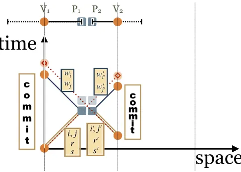
Fig. 2.Space-Time diagram of our ZK-MIP?forNP. (45◦diagonals are the speed of light. )
systemestablished by the two commitments and not by explicitly requesting anyone to unveil. This is the unveil-via-commit principle (very similar to the double-spending mechanism of the untraceable electronic cash of Chaum, Fiat and Naor[13]). We then use the Lemma of [11] to prove soundness of the three-prover version of this protocol even when the provers areentangled. A positive side of the protocol of [6], however, is the fact that only two provers are necessary while we use three. Zero-Knowledge follows from the fact that only two edge nodes can be unveiled by requesting the same edge to both provers. Otherwise only a single node may be unveiled. Finally, we show that even the three-prover version of this protocol retains the zero-knowledge property: requesting any three edges from the provers may allow the verifiers to unveil the colours of a triangle in the graph but never two end-points that do not form an edge (going to four provers would however defeat the zero-knowledge aspect).
An actual physical implementation of this protocol is currently being developed in collabo-ration with Pouriya Alikhani (McGill), Nicolas Brunner, S´ebastien Designolle, Weixu Shi, and Hugo Zbinden (Universit´e de Gen`eve).
1.1 Implementations Issues
Traditionally in the setup of Multi-Prover Interactive Proofs, there is a single verifier interacting with the many provers. However, when implementing no-communication via spatial separation (the so called relativistic setting) it is standard to break the verifier in a number of verifiers equal to the number of provers, each of them interacting at very short distance from their own prover. The verifiers can use the timing of the replies of their respective provers to judge their relative distance. In practice, this means that we can implement MIPs under relativistic assumptions if the verifier are “split” into multiple verifiers, each locally interacting with its corresponding prover. The verifiers use the distance betweenthemselves to enforce the impossibility of the provers to communicate: no message from a verifier can be used to reply to another verifier faster than the speed of lightwherever the provers are located.
Moreover, multi-prover interactive proof systems may have several rounds in addition to several provers. In general, protocols with several rounds may cause a treat to the inherent assumption that the provers are not allowed to communicate during the protocol’s execution. Nevertheless, most of the existing literature resolves this issue by providing an honest verifier that isnon-adaptive. To simplify this task, most of the protocols are actually single-round. We stick to these guidelines in this work. Moreover, in order to prove soundness of our protocols against entangled provers, we use a theorem that is currently only proven for single-round protocols. The protocols we describe are indeed single-round and non-adaptive.
2
Preliminaries
2.1 Notations
Random variables A, B ∈ Γ are said to be equivalent, denoted A = B, if for all x ∈ Γ, Pr (A=x) = Pr (B =x). The class of probabilistic polynomial-time Turing machines will be denoted PPT in the following. A PPT Turing machine is one having access to a fresh infinite read-only tape of random values (uniform values from the set of input symbols) at the outset of the computation. In the following, adversaries will also be allowed (in some cases) to be quantum machines. The precise ways quantum and classical machines are defined is not important in the following.
For M a Turing machine, we denote by M(x) it execution with x on its input tape (x
being a string of the tape alphabet symbols). A Turing machine (quantum or classical) aug-mented with read-only auxiliary-input tapes and write-only auxiliary-output tapes is called an
write-only output tapes allow to send messages. Interactive Turing machine M1 and M2 are said tointeract when for each of them, one of its write-only auxiliary-output tape corresponds to one read-only auxiliary-input tape of the other Turing machine. An execution of interactive Turing machines M1, . . . , Mk on common input x is denoted [M1. . . Mk](x). For 1 ≤ i ≤ k, machine Mi accepts the interactive computation on input x if it stops in state accept after the execution [M1. . . Mk](x). When the ITM Mi that accepts a computation is clear from the context, we say that [M1. . . Mk](x) accepts when Mi’s final state is accept. In this scenario, Pr ([M1. . . Mk](x) =accept) denotes the probability that Mi terminates in state accept upon common input x. Quantum machines are also interacting through communication tapes the same way than for classical machines. When a quantum machine M1 interacts with a classical machine M2, we suppose that the write-only auxiliary tape and the reade-only auxiliary tape of M1 used to communicate with M2 are classical. This is the situation we will be addressing almost all the time in the following. A quantum machineM is also allowed to have a quantum auxiliary read-only input tape that may contain a part of a quantum state shared with other machines. This allows to model machines sharing entanglement at the outset of an interactive computation. Henceforth, we suppose that the (main) input tape of all machines (quantum or classical) is classical.
In the following, G = (V, E) denotes an undirected graph with vertices V and edges E. If
n=|V|then we denote the set of vertices inGbyV ={1,2, . . . , n}. We suppose that (i, i)∈/E
for all 1 ≤i ≤n(i.e. Ghas no loop). We denote uniquely each edge in E as (i, j) withj > i. Fori∈V, letEdges(i) :={(j, i)∈E}j<i∪ {(i, j)∈E}j>i be the set of edges connecting vertex
iinG. Fore, e0∈E, we definee∩e0 =i∈V ifeande0 have only one vertexi∈V in common. Whene ande0 have four distinct vertices in V, we sete∩e0 = 0. Finally, whene=e0, we set
e∩e0 :=∞. For readability, we use the following special notations: (a, b)6=6= (c, d) means a6=c andb6=d, while as always, (a, b)6= (c, d) simply meansa6=c orb6=d.
2.2 Non-local Games, Multi-Prover Interactive Proofs, and Relativistic Proofs Multi-provers interactive protocols are protocols involving a set ofproversmodelled by interactive Turing machines, each of them interacting with an interactive PPT Turing machine called the verifierV. Although all provers may share an infinite read-only auxiliary input tape at the outset of their computation, they do not not interact with each other. When the provers are quantum, an extra auxiliary read-only quantum input tape is given and can be entangled with other provers at the beginning.
Definition 1. Let P1, . . . ,Pk be computationally unbounded interactive Turing machines and
let V be an interactive PPT Turing machine. The Pi’s share a joint, infinitely long, read-only
random tape (and an auxiliary reads-only quantum input tape if the provers are quantum). Each Pi interacts withV but cannot interact withPj for any 1≤j6=i≤k. We call [P1, . . . ,Pk,V] a
k-prover interactive protocol (k–prover IP).
A [P1, . . . ,Pk,V]k-prover interactive protocol is amulti-prover interactive proof system forL if it can be used to showVthat a public inputxis such thatx∈L. At the end of its computation, Vconcludesx∈Lif and only if it ends up in stateaccept. We restrict our attention to interactive proof systems with perfect completeness since all our protocols have this property.
Definition 2. The k–prover interactive protocol Π = (P1, . . . ,Pk,V) is said to be a k-prover interactive proof system with perfect completeness for L if there exists q(n)<1− 1
poly(n) such
that following holds:
perfect completeness: (∀x∈L)Pr [P1, . . . ,Pk,V](x) =accept
= 1,
soundness: (∀x /∈L)(∀Pe1, . . . ,ePk) h
Pr [eP1, . . . ,ePk,V](x) =accept
The parameter q(|x|) is called the soundness error of Π. Soundness can hold against classical provers or against quantum provers sharing entanglements. The former case is called sound against classical proverswhile to latter is called sound against entangled provers.
Consider ak–prover interactive proof systemΠ(x) (with or without perfect completeness) for
Lexecuted with public inputx /∈L. In this situation,Π(x) defines what is called aquantum game. The minimum valueq(|x|) such that for allP10, . . . ,P0k, Pr [P01, . . . ,P0k,V](x) =accept≤q(|x|) is often called the classical value of game Π[x] and is denoted ω(Π(x)) when the provers are restricted to be classical and unable to communicate with each other upon public inputx. When the provers, still unable to communicate with each other, are allowed to carry their computation quantumly and share entanglements, we denote by ω∗(Π(x)) ≥ ω(Π(x)) the minimum value
q(|x|) such that for all such quantum proversP0
1, . . . ,P0k, Pr [P01, . . . ,P0k,V](x) =accept
≤q(|x|). In this case,ω∗(Π(x)) is called the quantum value of game Π(x). Ak–prover interactive proof system for L is said to be symmetric if V can permute the questions to all provers without changing their distribution. The following result of Kempe, Kobayashi, Matsumoto, Toner, and Vidick[11] shows that the classical value of a symmetric one-round classical game cannot be too far from the quantum value of a modified game. Given a symmetric one-round two-prover gameΠ, one can always add a third proverP3 and Vasks P3 the same question thanP1 with probability 12 or the same question than P2 with probability 21. Then, V accepts if P1 and P2 would be accepted in Π(x) and if P3 returns the same answer than the one returned by the prover it emulates. We callΠ0(x) the modified game obtained that way fromΠ(x).
Lemma 1 ([11], Lemma 17). Let Π(x) be a two-prover one-round symmetric game and let
Π0(x) be its modified version with three provers. Ifω∗(Π0(x))>1−ε then ω(Π(x))>1−ε−
12|Q|√ε whereQis the set of V’s possible questions to a prover in Π.
Lemma 1 remains true for non-symmetric two-prover one-round protocol by first making them symmetric at the cost of increasing the size of Q. This is always possible without changing the classical value of the game and by using twice the number of questions|Q|of the original game (Lemma 4 in [11]).
Let [P1, . . . ,Pk,V] be a k–prover IP. We denote by view(P1, . . . ,Pk,V, x) the probability distribution ofV’s outgoing and incoming messages with all provers accordingV’s coin tosses.
Definition 3. Let [P1, . . . ,Pk,V] be a k-prover interactive proof system for L. We say that [P1, . . . ,Pk,V]isperfect zero-knowledgeif for allPPTinteractive Turing machinesVethere exists
aPPTmachine Sim(i.e. the simulator) having blackbox access toVe such that for all x,
view(P1, . . . ,Pk,Ve, x) =Sim(x) ,
and both random variables are equivalent. In the following, we allow Ve to be a quantum
ma-chine but our simulators will always be classical mama-chines with blackbox access to Ve. If the
zero-knowledge condition holds against quantumVe, we say that the proof system is perfect zero-knowledge against quantum verifiers.
2.3 Multi-Prover Commitments with Implicit Unveiling
Our multi-prover proof systems for3COLuse a simple 2-committer commitment scheme with a property allowing to guarantee perfect zero-knowledge. In this section, we give the description of this simple commitment scheme with its important properties four our purposes.
Assume that proversP1andP2share`valuesc1, c2, . . . , c`∈FwhereFis a finite set.Vwants
to check that these values satisfy some properties without revealing them all. Assume thatFis
Bit commitment schemes have been used in the multi-prover model ever since it was intro-duced in [2]. The original scheme was basicallywi:=bi·ri+ci, a commitmentwi to valueci∈F
using pre-agreed random maskbi ∈RF and randomnessri6= 0 provided byV. Kilian[14] had a binary version where each bitci:=c1i⊕c2i⊕c3i is shared among proversP1andP2(and therefore
F needs only to be a group). To commitci, V sampleschi from P1 and cji from P2 at random. If j =h but cji 6= chi, V immediately rejects the commitment. Otherwise either P1 or P2 may unveil by disclosingc1
i, c2i, c3i at a later time. Somehow, bad recollection of [2]’s scheme lead [15] to a similar but different scheme defining wi :=ci·ri+bi, a commitment wi to bitci ∈ {0,1} using pre-agreed bit maskbi ∈R{0,1}and binary randomnessriprovided by their corresponding verifiers. Although this form of commitment is intimately connected to the CHSH game [16] and the Popescu-Rohrlich box[17], this proximity is not relevant for the soundness and the complete-ness of our protocols, even against entangled provers. Although the (limited) binding property of these schemes has been established in [3, 18, 5, 19, 4, 6] against entangled provers, we only use this commitment scheme against classical provers, only sharing classical information before the execution of the protocol. The weak binding property of these schemes against entangled provers does not allow us to get sound and complete proof systems against these provers. We shall rather get completeness and soundness against entangled provers using a different technique from [11] that requires a third prover.
For an arbitrary field F, the commitment scheme produces commitment wi :=ci·ri+bi to field element ci ∈ F using pre-agreed field element mask bi (specific to value 1 ≤ i ≤ `) and random field elementri6= 0 provided by their corresponding verifiers. Many results were proven for this specific form of the commitments. Notice however that the two versions discussed above,
wi :=bi·ri+ci in the former case and wi :=ci·ri+bi in the latter have equivalent binding property(left as a simple exercice). Considering, the former as being the degree-one secret sharing [20] ofci hidden in the degree zero term, while the latter being the degree-one secret sharing of
ci hidden in the degree one term, we decided to use the former (original BGKW form) because all the known results about secret sharing are generally presented in this form. In particular, this form is more adapted to higher degree generalizations such aswi:=ai·ri2+bi·ri+cibeing the degree-two secret sharing ofci hidden in the degree zero term, and so on.
Moreover, this choice turns out to simplify our (perfect) zero-knowledge simulator. For the rest of this paper, we use wi :=bi·ri+ci where wi, bi, ci ∈F3 andri ∈ F∗3. Provers therefore commit to trits, one value for each node corresponding to its colour in a 3–colouring of graph
G= (V, E). The values shared betweenP1 andP2 are therefore, for each nodei∈V, the colour
ci of that node.
Suppose thatVasksP1to commit on the colourciof nodei∈V using randomnessr∈RF∗3. Letw =bi·r+ci be the commitment returned toV by P1. SupposeV asks P2 to commit on the colourc0
j of nodej∈V using randomnessr0 ∈RF∗3. Letw0=bj·r0+c0j be the commitment issued toVbyP2. The following 3 cases are possible depending onV’s choices fori, j, r, andr0:
1. (forever hiding) ifi6=jthenVlearns nothing on neithercinorc0j sincewandw0 hideciand
c0jwith random and independent masksbi·randbj·r0respectively. Even knowingr, r0∈F∗3,
bi·r andbj·r0 are uniformly distributed inF3.
2. (the consistency test) Ifi=jandr=r0thenVcan verify thatw=w0. This corresponds to the immediate rejection of Vin Kilian’s two-prover commitment described above. It allows Vto make sure that P1 andP2are consistant when asked to commit on the same value.
3. (implicit unveiling) If i =j and r0 6= r then V can learn ci (assuming w =bi·r+ci and
As long as P1 and P2 arelocal (or quantum non-local) they cannot distinguish which option V has picked among the three. The consistency test makes sure that ifP1 andP2 do not commit on identical values for some 1≤i≤`thenVwill detect it whenVpicks the consistency test for commitmentwandw0 in positioni.
3
Classical Two-Prover Protocol
First, consider a small variation over the protocol of Cleve et al. presented in [12]. In their protocol, whenP1andP2both know and act upon the same valid 3-colouring ofG,Vasks each prover for the colour of a vertex in G= (V, E). Consistency is verified when V asks the same vertex to each prover and compares that the same colour has been provided. The colorability is checked when the provers are asked for the colour of two connected vertices inG. This way of proceeding is however problematic for the zero-knowledge condition. V could be asking two nodes that do not form an edge for which their respective colour will be unveiled. This certainly allowsV to learn something about P1’s and P2’s colouring. Indeed, repeating this many times will allowVto efficiently reconstruct a complete colouring. To remedy partially this problem,V is instead asking each prover the colouring of an entire edge ofG. The colouring is (only) checked when both provers are asked the same edge, while consistency is checked when two intersecting edges are asked to the provers.
3.1 Distribution of questions
Let G = (V, E) be a connected undirected graph. Let us define the probability distribution
DG ={(p(e, e0),(e, e0))}e,e0∈E for the pair (e, e0)∈E×E that V picks with probabilityp(e, e0)
before announcingetoP1ande0 toP2. Fore, e0 ∈E such thate∩e0= 0, we setp(e, e0) := 0 so thatVnever asks two disconnected edges inG(this would give no useful information).
The first thing to do is to picke= (i, j)∈E uniformly at random. With probability(to be selected later), we sete0 =e, which allows for an edge-verification test. With probability 1−, we perform a well-definition test as follows. With probability 1
2,e
0 ∈Edges(i) uniformly at random
and with probability 1 2, e
0 ∈ Edges(j) uniformly at random. In other words, the well-definition
test picks the second edge e0 with probability 1
2 among the edges connecting i ∈ V and with probability 12 among the edges connectingj∈V. It follows that fore0 ∈Edges(i)∪Edges(j) with
e6=e0, we have, fore= (i, j)∈E,
p(e, e0) = 1− 2|E|
|{e0} ∩Edges(i)|
|Edges(i)| +
|{e0} ∩Edges(j)| |Edges(j)|
. (1)
We also get
p(e, e) =
|E|+
1−
2|E|
1
|Edges(i)|+
1
|Edges(j)|
≥
|E| . (2)
It is easy to verify thatDG is a properly defined probability distribution over pairs of edges.
3.2 A Variant Over the Two-Prover Protocol of Cleve et al.
Protocol Πstd(2)[G] : Two-prover, 3-COL.
Provers P1,P2 pre-agree on a random 3-colouring of G: {(i, ci)|ci∈ F3}i∈V such that (i, j)∈E =⇒ cj6=ci.
Interrogation phase:
– Vpicks ((i, j),(i0, j0))∈DGE×E, sends (i, j) toP1and (i
0, j0) toP
2. – If (i, j)∈E thenP1replies withci, cj.
– If (i0, j0)∈E thenP2replies withci0, cj0.
Check phase:
– Edge-Verification Test:
if (i, j) = (i0, j0) thenVaccepts iffci=ci0 6=cj0 =cj.
– Well-Definition Test:
if (i, j)∩(i0, j0) =h∈V thenVaccepts iffch=c0h.
The perfect soundness of this protocol is not difficult to establish along the same lines of the proof of soundness for the original protocol in [12]. On the other hand, zero-knowledge does not even hold against honest verifiers.V learns the colour of each node contained in any two edges of G. This is certainly information about the colouring thatV learns after the interaction. To some extend, the modifications we applied to the 2-prover interactive proof system of [12] leaks even more to V. In the next section, we show that the 2-prover commitment scheme, that we introduced in Sect. 2.3, can be used in protocolΠstd(2) to prevent this leakage completely.
4
Perfect Zero-Knowledge Two-Prover Protocol
We modify the protocol of section 3.2 to preventV from learning the colours of more than two connected nodes inG. The idea is simple,P1andP2 will return commitments for the colours of the nodes asked byV. The implicit unveiling of the commitment scheme described in section 2.3 will allowVto perform both the edge-verification and well-definition tests in a very similar way that in protocol Πstd(2). The commitments require V to provide a random nonzero trit for each node of the edge requested to a prover.
4.1 Distribution of questions
We now define the probability distributionD0
G for V’s questions in protocolΠ (2)
loc[G] defined in the following section. It consists in one edge and two nonzero trits for each prover:
D0
G={(p0(e, r, s, e0, r0, s0),((e, r, s),(e0, r0, s0))}e,e0∈E,r,s,r0,s0∈ F∗3
upon graphG= (V, E) and where (e, r, s) is the question toP1 and (e0, r0, s0) is the question to
P2.D0G is easily derived from the distributionDG ={(p(e, e0),(e, e0))}e,e0∈E for the questions in
Πstd(2)[G], as defined in section 3.1. First, an edgee∈REis picked uniformly at random. Together with e, two nonzero trits r, s∈R F∗3 are picked at random. Then, as in DG, with probability (to be selected later) the second edgee0=e, in which case we always setr0 =−rands0 =−s. This case allows for an edge-verification test. Finally, with probability 1−, we pick e0 with probability p(e, e0) and pickr0, s0 ∈R F∗3 so that the couple ((e, r, s),(e0, r0, s0)) is produced with probability 161p(e, e0) for alle, e0∈E, andr, s, r0, s0 ∈F∗3. This will allow for a well-definition test. A consequence of (1) is that fore= (i, j)∈E,e0 ∈Edges(i)∪Edges(j) withe6=e0,
p0(e, r, s, e0, r0, s0)≥ 1−
16|E|
|{e0} ∩Edges(i)|
|Edges(i)| +
|{e0} ∩Edges(j)| |Edges(j)|
According to (2), we also get
p0(e, r, s, e, r, s) =p(e, e)
4 ≥
4|E| . (4)
It is easy to verify thatD0
G is a properly defined probability distribution.
4.2 The Protocol
The protocol is similar to Πstd(2) except that instead of returning to V the colour for each node of an edge inG, each prover returns commitments with implicit unveilings of these colours. IfV asks two disjoint edges thenVlearns nothing about the values committed by theforever-hiding
property of the commitment scheme. The resulting 2–prover one-round interactive proof system is denotedΠloc(2).
Protocol Πloc(2)[G] : Two-prover, 3-COL
P1andP2pre-agree on random masksbi∈RF3for eachi∈V and a random 3-colouring ofG:{(i, ci)|ci∈F3}i∈V such that (i, j)∈E =⇒ cj 6=ci.
Commit phase:
– V picks (((i, j), r, s),((i0, j0), r0, s0)) ∈D0
G E×(F
∗
3)2 2
, sends ((i, j), r, s) to P1 and ((i0, j0), r0, s0) toP2.
– If (i, j)∈E thenP1replieswi=bi·r+ci andwj =bj·s+cj. – If (i0, j0)∈E thenP2repliesw0i0 =bi0·r0+ci0 andw0j0 =bj0·s0+cj0.
Check phase:
Edge-Verification Test:
– if (i, j) = (i0, j0) and (r0, s0)6=6= (r, s) thenVaccept iffw
i+w0i6=wj+w0j. Well-Definition Test:
– If (i, j) = (i0, j0) and ¬((r0, s0)6=6= (r, s)) thenV accepts iff ((wi =w0i)∨(r 6= r0))∧ ((wj=w0j)∨(s6=s0)).
– if (i, j)∩(i0, j0) =iandr0=rthenVaccepts iff wi=w0i. – If (i, j)∩(i0, j0) =j ands0=sthenVaccepts iffwj =w0j.
Clearly,Πloc(2)satisfies perfect completeness. The following theorem establishes that in addition
to perfect completeness,Πloc(2) is sound against classical provers.
Theorem 1. The two-prover interactive proof system Πloc(2) is perfectly complete with classical valueω(Πloc(2)[G])≤1− 1
12·|E| upon any graph G= (V, E)∈/3COL.
Proof. Perfect completeness is obvious. AssumeG /∈3COLand let us consider the probabilityδ
thatVdetects an error in the check phase when interacting with two local dishonest provers ˜P1 and ˜P2. Π
(2)
loc is a one-round protocol where the provers cannot communicate directly with each other nor through V’s questions since they are independent of the provers’ answers. It follows that the strategy of ˜P1and ˜P2can be made deterministic without damaging the soundness error by letting each prover choosing the answer that maximizes her/his probability of success given her/his question. Therefore, consider a deterministic strategy as a pair of arraysW`[i, r, j, s]∈F23 to be used by prover ˜P` for ` ∈ {1,2} (i.e. we only care about the entries where (i, j)∈E upon question ((i, j), r, s)). For z∈ {1,2}, Wz`[·,·,·,·] is the z-th component of the output pair
given to a prover is irrelevant (V can always choose the same order). We say that W[i, r] for [i, r]∈E×F∗3is well defined if for allj, ksuch that (i, j),(i, k)∈Edges(i)6=∅and∀s, t∈F∗3,
W11[i, r, j, s] =W12[i, r, k, t] . (5)
ForW[i, r] well defined, we setW[i, r] :=W1
1[i, r, j,1] for an arbitraryjsuch that (i, j)∈Edges(i). We now lower bound the probabilityδwdt>0 that, whenW[i, r] is not well-defined for some
i ∈ V and r ∈ F∗3, the well-definition test will detect it. When (5) is not satisfied , we have
W1
1[i, r, j, s]6=W12[i, r, k, t] for some (i, j),(i, k)∈Edges(i). Lete= (i, j) ande0= (i, k) be these two edges. According to (3) (and (1) whene =e0), the well-definition test will then detect an error with probability
Pr (Vpickseande0 with randmonessr, s, t) =p0(e, r, s, e0, r, t)≥ 1−
16· |E||Edges(i)| . (6)
We can do much better. ConsiderW1
1[i, r, m, u], W12[i, r, m, u] for (i, m)∈Edges(i) and u∈F∗3. Fori∈V and and valuer∈F∗3 fixed, three cases can happen:
1. W1
1[i, r, m, u] 6= W12[i, r, k, t], in which case e = (i, m) and e0 = (i, k) are incompatibe for valuesuandt, or
2. W1
1[i, r, j, s] 6= W12[i, r, m, u], in which case e = (i, j) and e0 = (i, m) are incompatible for valuessandu, or
3. W1
1[i, r, m, u] =W12[i, r, k, t] andW12[i, r, m, u] =W11[i, r, j, s], in which case W11[i, r, m, u]6=
W2
1[i, r, m, u] and e=e0 = (i, m) are incompatible for valueuon both sides.
In other words, if (i, j),(i, k)∈Edges(i) are such that W1
1[i, r, j, s]6=W12[i, r, k, t] then for any (i, m)∈Edges(i) and for any randomnessu∈F∗3associated to nodem,Vcatches the provers with probability expressed on the right hand side of (6). It follows that ifW[i, r] is not well defined then there are 2· |Edges(i)|ways forVto catch the provers and each of these has probability at least 16·|E|·|1−Edges (i)| to be picked. It follows that,
δwdt≥
2(1−)· |Edges(i)|
16· |E| · |Edges(i)| =
1−
8· |E| .
Now, assume that for all i ∈ E and r ∈ F∗
3, W[i, r] is well-defined, which means that the commitment values produced by the provers satisfy the consistency test. As discussed in section 2.3, when the commitments are consistent, the unique values committed upon are defined by
ci := 2−1·(W[i, r] +W[i,−r]). Since G /∈3COL, two of the nodes must be of the same colour at the end-points of at least one edge (i∗, j∗) ∈ E. In this case the edge-verification test will detect it when (i∗, j∗) is the edge announced to both provers and if randomness (r, s)∈F∗3×F∗3 is announced toP1 then (−r,−s) is the randomness announced to ˜P2. Using (4), the probability
δevt to detect such an edge whenW[i, r] is well defined for alli∈V andr∈F∗3 satisfies
δevt≥min e∈E(p
0(e, r, s, e, r, s))≥
4· |E| .
Therefore, the detection probabilityδof any deterministic strategy forG /∈3COLsatisfies
δ≥min(δwdt, δevt)≥ 1
12· |E| (maximized at= 1/3) .
To prove (perfect) zero-knowledge, it suffices to show that if ((i, j), r, s) and ((i0, j0), r0, s0) are selected arbitrarily, Vcan determine at most the colours of two nodes (that form an edge). The commitments prevent a dishonest prover eVto learn the colours of two nodes that are not connected by an edge inG. Proving this is not very hard and will be done in Section 5.3 for the three-prover case (although with three provers,Ve may also learn the colour of three nodes that form a triangle). The addition of a third prover will allow, using lemma 1, to get soundness against entangled provers without compromising zero-knowledge. As shown in [12], their protocol is not necessarily sound against two entangled provers. We also do not know whether Πstd(2) is sound against two entangled provers.
5
Three-Prover Protocol Sound Against Entangled Provers
The three-prover protocol Πqnl(3), defined below, is identical to Πloc(2) except thatP3 is asked to repeat exactly what P1 or P2 has replied. The prover that P3 is asked to emulate is picked at random by V. An application of lemma 1 allows to conclude the soundness of Πqnl(3) against entangled provers. Zero-knowledge remains since the only way to provideVwith the colours of more than two connected nodes is if they form a complete triangle ofG. This reveals nothing beyond the fact thatG∈3COLto V, since all nodes will then show different colours.
5.1 Distribution of questions The probability distributionD00
GforV’s questions to the three provers is easily obtained from the distributionDG0 for the questions in protocolΠloc(2)[G].Vpicks ((e, r, s),(e0, r0, s0))∈D0
G E×(F
∗
3)2 2
and setse00=e,r00=r, ands00=swith probability 12 or setse00=e0,r00=r0, ands00=s0 also with probability 12. Defined that way, D00
G is a properly defined probability distribution for V’s three questions, each one inE×(F∗3)2.
5.2 The Protocol
Protocol Πqnl(3)[G] : Three-prover, 3-COL.
ProversP1,P2, and P3 pre-agree on random values bi∈RF3for alli∈V and a random 3-colouring of G:{(i, ci)|ci∈ {0,1,2}}i∈V such that (i, j)∈E =⇒ cj 6=ci.
Commit phase:
– Vpicks (((i, j), r, s),((i0, j0), r0, s0),((i00, j00), r00, s00))∈D00
G E×(F
∗
3)2 3
, sends ((i, j), r, s) toP1, sends ((i0, j0), r0, s0) toP2, and sends ((i00, j00), r00, s00) toP3.
– If (i, j)∈E thenP1replieswi=bi·r+ci andwj =bj·s+cj. – If (i0, j0)∈E thenP2repliesw0i0 =bi0·r0+ci0 andw0j0 =bj0·s0+cj0.
– If (i00, j00)∈E thenP3repliesw00i00=bi00·r00+ci00 andw00j00 =bj00·s00+cj00.
Check phase:
Consistency Test:
– If ((i00, j00), r00, s00) = ((i, j), r, s) thenVrejects if (wi, wj)6= (w00i00, wj0000).
– If ((i00, j00), r00, s00) = ((i0, j0), r0, s0) thenVrejects if (wi00, w0j0)6= (wi0000, w00j00).
Edge-Verification Test:
– if (i, j) = (i0, j0) and (r0, s0)6=6= (r, s) thenVaccept iffw
i+w0i6=wj+w0j. Well-Definition Test:
In protocolΠqnl(3), after the three questions picked accordingD00
G byVhave been answered by the the provers,Vaccepts if and only if the replies ofP1andP2are accepted inΠ
(2)
loc and in addition,
P3 gave the same reply than the prover it emulates.
The soundness of protocolΠqnl(3) against entangled provers can easily be shown a direct
conse-quence of the soundness of protocolΠloc(2) against classical provers, by an application of Lemma 1. Indeed, the soundness error corresponds to the quantum value of the game whenG /∈3COLand
Πloc(2) is obviously symmetric.
Theorem 2. The three-prover interactive proof systemΠqnl(3) is perfectly complete and has quan-tum value
ω∗(Πqnl(3)[G])≤1−
1
25|E|
4
(7)
upon any graphG= (V, E)∈/3COL.
Proof. Assume G = (V, E) ∈/ 3COL. The contrapositive of Lemma 1 indicates any one-round symmetric game Πloc(2)[G] with classical value ω(Πloc(2)[G]) ≤ 1−δ−12|Q|√δ is such that the modified game Πqnl(3)[G] has quantum value ω∗(Πqnl(3)[G]) ≤ 1−δ. The set Q of questions to
each player satisfies|Q|= 4|E|. Theorem 1 establishes that δ+ 12|Q|√δ≥ 1
12|E|, which implies
√
δ≥ 1
(1+12|Q|)·12·|E| =
1
12|E|+576|E|2 ≥
1
588|E|2, and the result follows.
As an immediate consequence of Theorem 2,Ω(|E|4) sequential repetitions ofΠ(3)
qnl produces an interactive proof system for 3COL with negligible soundness error. Although the resulting proof system can be implemented on short distances, these many sequential communication rounds need to be performed at high rate for a given proof to be concluded in reasonable time. A few executions ofΠqnl(3) could be run in parallel without having to increase (significantly) the distances while reducing the number of sequential rounds. However, we don’t know how the soundness error decreases whenΠqnl(3) is run only a few times in parallel, even though the results of Kempe and Vidick, a quantum version of Raz’s parallel repetition theorem[21], indicate that
Ω(|E|4) runs in parallel produces a proof system with negligible soundness error[22].
5.3 Proof of Perfect Zero-Knowledge
In this section, we prove that protocolΠqnl(3)is perfect zero-knowledge. As a consequence,Πloc(2) is
also zero-knowledge since everything Ve sees in Π (2)
loc can also be observed inΠ (3)
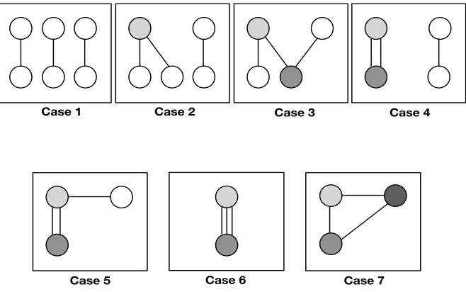
qnl. The proof of zero-knowledge proceeds using the fact that a vertex must appear at least twice to have its colour unveiled. This is theforever hiding property of the commitment scheme described in Section 2.3. Notice that this would be enough for Ve to learn something about the colouring if no extra condition on these three vertices is observed. In fact, we can easily show that only a few cases of colour disclosure are possible and in each of these cases,Ve learns nothing about the colouring that it could not have computed on its own.Ve can only learn colour of two connected vertices in
Gand nothing else or the colours of three vertices forming a triangle inG. In each of these cases,
e
these vertices, the committed values received from the provers are just random and independent elements inF3. In each of the 7 cases, the unveiled colours of the vertices are displayed in shade of grey. We see that the only way to unveil the colour of two vertices (cases 2, 3, 4, 5, and 6) is when they are connected by an edge, which means that the colours of both vertices are random but distinct. The only way for Ve to learn the colour of 3 distinct vertices is when they form a triangle (case 7). In this case,Ve learns three random and distinct colours. Clearly, this is nothing more than something necessarily true whenG∈3COL.
These properties of the commitment scheme allows, for any quantum polynomial-time dis-honest verifierVe, an easy simulator forview(P1,P2,P3,Ve, G) whenG∈3COL, thus establishing thatΠqnl(3) is perfect zero-knowledge.
Theorem 3. The three-prover interactive proof system Πqnl(3) is perfect zero-knowledge against quantum verifiers.
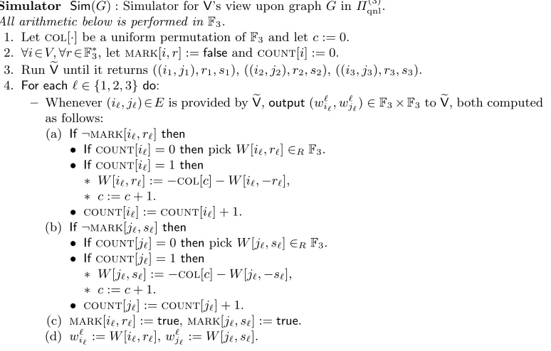
Proof. The simulator Sim, see Fig. 3, is classical given blackbox access to Ve (and Ve can be quantum). Consider an execution Sim(G) upon graph G= (V, E). It first picks a random per-mutation col[·] : F3 7→ F3 over three colours, each corresponding to a distinct element in F3. Tablemark[i, r]∈ {true,false}, fori∈V andr∈F∗3, is initialized tofalseand will indicate if the output of a prover has already been simulated for vertexi with randomnessr. Tablecount[i], for i ∈ V, counts the number of times vertex i has been asked so far during the simulation. Variablec∈F3, initialized to 0, indicates the next colour index the simulator should use when a new colour must be unveiled during the simulation.
Simulator Sim(G) : Simulator foreV’s view upon graphGinΠ
(3) qnl. All arithmetic below is performed inF3.
1. Letcol[·] be a uniform permutation ofF3 and letc:= 0. 2. ∀i∈V,∀r∈F∗3, letmark[i, r] :=falseandcount[i] := 0.
3. RunVeuntil it returns ((i1, j1), r1, s1), ((i2, j2), r2, s2), ((i3, j3), r3, s3). 4. For each`∈ {1,2,3}do:
– Whenever (i`, j`)∈Eis provided byV,e output(wi``, w `
j`)∈F3×F3toV, both computede
as follows:
(a) If¬mark[i`, r`]then
• Ifcount[i`] = 0thenpickW[i`, r`]∈RF3.
• Ifcount[i`] = 1then
∗ W[i`, r`] :=−col[c]−W[i`,−r`],
∗ c:=c+ 1.
• count[i`] :=count[i`] + 1. (b) If¬mark[j`, s`]then
• Ifcount[j`] = 0thenpickW[j`, s`]∈RF3.
• Ifcount[j`] = 1then
∗ W[j`, s`] :=−col[c]−W[j`,−s`],
∗ c:=c+ 1.
• count[j`] :=count[j`] + 1.
(c) mark[i`, r`] :=true,mark[j`, s`] :=true. (d) w`
i` :=W[i`, r`],w `
j` :=W[j`, s`].
e
Vis then invoked to produce questions ((i`, j`), r`, s`) for all proversP`, `∈ {1,2,3}.Simnow aims at setting the values (w`
i`, w
`
j`) forP`’s commitments. If (i`, j`)∈/E,Simproduces no value for (w`
i`, w
`
j`), exactly asP` inΠ
(3) qnl.
When (i`, j`)∈E,Simfirst producesP`’s commitmentwi`` fori`∈V and then producesP`’s commitmentw`
j` for j` ∈ V. We show how to compute w
` i`, w
`
j` is computed similarly mutatis mutandis:
– if mark[i`, r`] then Sim returns the value of w`i` already determined for the simulation of the commitment of an earlier prover Ph, h < `. This ensures that both the commitment’s
consistency test performed and the well-definition test are always successful, as inΠqnl(3) with honest provers.
– if¬mark[i`, r`] thenSimhas never simulated a commitment of the colour for vertexi`with randomnessr`. The valuecount[i`] indicates the number of time prior to this value for `, vertex i`has been asked:
• Ifcount[i`] = 0 thenw`i` ∈RF3is picked uniformly at random, as it should be when the
commitment value for the colour of vertexi` is observed in isolation.
• Ifcount[i`] = 1 then the colour associated to vertexi`has been committed to valuewhi`
by anearliersimulated proverPh,h < `upon randomness−r`(otherwise,mark[i`, r`] =
true).Simsetsw`
i` =−col[c]−w
h
i`, which satisfies theimplicit unveilingof random colour col[c] =−w`i`−whi`. The current colourcis incremented.
The value ofcount[i`] is increased by one andmark[i`, r`] =true, as the colour of vertexi` with randomnessr`has been committed upon by the simulated proverP`.
Let (w1 i1, w
1 j1), (w
2 i2, w
2
j2), and (w
3 i3, w
3
j3) be all commitment values simulated by Sim. As
discussed above and shown in Fig. 4, the colours of no more than 3 vertices are unveiled in the process. Sim always unveils as many different colours there are colours unveiled to Ve. If Sim’s simulated committed values unveils only the colour of one vertex then that colour is random, as it should in this case inΠqnl(3). IfSim’s committed values unveils the colours of exactly 2 vertices then these 2 vertices form an edge in Gand the colours are two different random colours, as it should be inΠqnl(3). Finally, whenSim’s committed values unveil the colours of exactly 3 vertices
then these vertices form a triangle inG. The 3 colours unveiled by Simto Ve are different and assigned randomly to each of the 3 vertices, as it is inΠqnl(3). Otherwise, ifw`
i fori∈V has been generated with only one random value thenw`
i is random and uniform inF3, exactly as it is in
Πqnl(3) in the same situation. It is now clear that,
view(P1,P2,P3,Ve, G) =Sim(G) ,
andΠqnl(3) is perfect zero-knowledge.
6
Conclusion and Open Problems
We have provided a three-prover perfect zero-knowledge proof system for NP sound against entangled provers that is implementable in some well controlled environment. In order to make it fully practical, it would be better to find a protocol with smaller soundness error and also requiring only two provers. Is it possible? Moreover, we would like to extend our techniques to prove any language inQCMAorQMA, the natural quantum extensions ofNP. We would also want to prove whetherΠstd(2)is sound against entangled provers. Finally, we seek a variant ofΠstd(2)
Case 1 Case 2 Case 3 Case 4
Case 5 Case 6 Case 7
Fig. 4.The 7 ways to unveil the colours of at most 3 nodes inΠqnl(3).
Acknowledgements
We would like to thank P. Alikhani, N. Brunner, S. Designolle, A. Chailloux, A. Leverrier, W. Shi, T. Vidick, and H. Zbinden for various discussions about earlier versions of this work. We would also like to thank Jeremy Clark for his insightful comments.
References
1. J. Kilian, “Strong separation models of multi prover interactive proofs,” inDIMACS Workshop on Cryptography, 1990.
2. M. Ben-Or, S. Goldwasser, J. Kilian, and A. Wigderson, “Multi-prover interactive proofs: How to remove intractability assumptions,” in Proceedings of the Twentieth Annual ACM Symposium on Theory of Computing, STOC ’88, (New York, NY, USA), pp. 113–131, ACM, 1988.
3. A. Kent, “Unconditionally secure bit commitment,”Phys. Rev. Lett., vol. 83, pp. 1447–1450, Aug 1999.
4. T. Lunghi, J. Kaniewski, F. Bussi`eres, R. Houlmann, M. Tomamichel, S. Wehner, and H. Zbinden, “Practical relativistic bit commitment,”Phys. Rev. Lett., vol. 115, p. 030502, Jul 2015.
5. E. Verbanis, A. Martin, R. Houlmann, G. Boso, F. Bussi`eres, and H. Zbinden, “24-hour relativistic bit commitment,”Phys. Rev. Lett., vol. 117, p. 140506, Sep 2016.
6. A. Chailloux and A. Leverrier, “Relativistic (or 2-prover 1-round) zero-knowledge protocol for NP secure against quantum adversaries,” inAdvances in Cryptology – EUROCRYPT 2017: 36th Annual International Conference on the Theory and Applications of Cryptographic Techniques, Paris, France, April 30 – May 4, 2017, Proceedings, Part III, pp. 369–396, Springer International Publishing, 2017. 7. D. Lapidot and A. Shamir, “A one-round, two-prover, zero-knowledge protocol for NP,”
Combina-torica, vol. 15, no. 2, pp. 204–214, 1995.
8. U. Feige and J. Kilian, “Two prover protocols: low error at affordable rates,” in Proceedings of the Twenty-Sixth Annual ACM Symposium on Theory of Computing, 23-25 May 1994, Montr´eal, Qu´ebec, Canada(F. T. Leighton and M. T. Goodrich, eds.), pp. 172–183, ACM, 1994.
10. A. B. Grilo, W. Slofstra, and H. Yuen, “Perfect zero knowledge for quantum multiprover interactive proofs,”Electronic Colloquium on Computational Complexity (ECCC), vol. 26, p. 86, 2019. 11. J. Kempe, H. Kobayashi, K. Matsumoto, B. Toner, and T. Vidick, “Entangled games are hard to
approximate,”SIAM Journal on Computing, vol. 40, no. 3, pp. 848–877, 2011.
12. R. Cleve, P. Høyer, B. Toner, and J. Watrous, “Consequences and limits of nonlocal strategies,” in Proceedings of the 19th IEEE Annual Conference on Computational Complexity, CCC ’04, (Wash-ington, DC, USA), pp. 236–249, IEEE Computer Society, 2004.
13. D. Chaum, A. Fiat, and M. Naor, “Untraceable electronic cash,” in Proceedings on Advances in Cryptology, CRYPTO ’88, (Berlin, Heidelberg), pp. 319–327, Springer-Verlag, 1990.
14. J. Kilian,Uses of randomness in algorithms and protocols. MIT Press, 1990.
15. G. Brassard, C. Cr´epeau, D. Mayers, and L. Salvail, “Defeating classical bit commitments with a quantum computer.” arXiv:quant-ph/9806031, June 1998.
16. J. F. Clauser, M. A. Horne, A. Shimony, and R. A. Holt, “Proposed experiment to test local hidden-variable theories,”Phys. Rev. Lett., vol. 23, pp. 880–884, Oct 1969.
17. S. Popescu and D. Rohrlich, “Quantum nonlocality as an axiom,”Foundations of Physics, vol. 24, no. 3, pp. 379–385, 1994.
18. C. Cr´epeau, L. Salvail, J.-R. Simard, and A. Tapp, “Two provers in isolation,” in Advances in Cryptology – ASIACRYPT 2011: 17th International Conference on the Theory and Application of Cryptology and Information Security, Seoul, South Korea, December 4-8, 2011. Proceedings, (Berlin, Heidelberg), pp. 407–430, Springer Berlin Heidelberg, 2011.
19. S. Fehr and M. Fillinger, “Multi-prover commitments against non-signaling attacks,” inAdvances in Cryptology – CRYPTO 2015: 35th Annual Cryptology Conference, Santa Barbara, CA, USA, August 16-20, 2015, Proceedings, Part II, (Berlin, Heidelberg), pp. 403–421, Springer Berlin Heidelberg, 2015.
20. A. Shamir, “How to share a secret,”Commun. ACM, vol. 22, no. 11, pp. 612–613, 1979.
21. R. Raz, “A parallel repetition theorem,”SIAM Journal on Computing, vol. 27, no. 3, pp. 763–803, 1998.
![Fig. 1. Space-Time diagrams of [6]’s ZK-MIPthe answers they get fromandthe number of nodes (and thus increasing the total commit time) pushes the verifiers further away fromIn the above two diagrams,to commit an entry of the adjacency matrixchall V⋆ for NP](https://thumb-us.123doks.com/thumbv2/123dok_us/7989416.1325964/2.612.104.523.80.329/diagrams-mipthe-fromandthe-increasing-veriers-diagrams-adjacency-matrixchall.webp)