Parallel (probable) lock-free HashSieve: a practical sieving algorithm for the SVP

Parallel (probable) lock-free HashSieve: a practical sieving

algorithm for the SVP

Artur Mariano

Computing Technische Universität

Darmstadt Darmstadt, Germany

[email protected]

Thijs Laarhoven

and Computer Science Eindhoven University of

Technology

Eindhoven, The Netherlands

[email protected]

Christian Bischof

Computing Technische Universität

Darmstadt Darmstadt, Germany

[email protected]

ABSTRACT

In this paper, we assess the practicability of HashSieve, a recently proposed sieving algorithm for the Shortest Vector Problem (SVP) on lattices, on multi-core shared memory systems. To this end, we devised a parallel implementation that scales well, and is based on a probable lock-free sys-tem to handle concurrency. The probable lock-free syssys-tem, implemented with spin-locks and compare-and-swap opera-tions, acts, likely, as a lock-free mechanism, since threads block only when strictly required and chances are that they are not required to block, because resource contention is very low. With our implementation, we were able to solve the SVP on an arbitrary lattice in dimension 96, in less than 17.5 hours, using 16 physical cores. The least squares fit of the execution times of our implementation, in seconds, lies between 2(0.32n−15)or 2(0.33n−16), which indicates that siev-ing algorithms are indeed way more practical than believed.

1.

INTRODUCTION

Cryptography is mainly used to protect information that is sent over an insecure channel. In the late 90s, Ajtai dis-covered that certain lattice problems have interesting prop-erties for cryptography, such as average-case hardness, and that lattices can be used for building cryptographic primi-tives [2]. At that point, the news had already broken that several classical cryptographic schemes (such as RSA) were insecure against quantum computers [22]. This led many re-searchers to engage on an intensive investigation of lattice-based alternatives for classical schemes, as these are believed to be, among others, secure against quantum attacks. One of the many discoveries in the field of lattice cryptography since then is that lattices can be used to construct the “holy grail” of cryptography, Fully Homomorphic Encryption [9], which made lattice-based cryptography one of the most prominent and rapidly growing fields of quantum resistant (also known as post-quantum) cryptography.

.

Cryptosystems (also called schemes in the cryptography world) are generally built on problems known to be hard. To estimate the actual computational complexity of these prob-lems in practice is of prime importance, because the param-eters of cryptosystems are chosen based on this complexity. Overestimating the computational complexity of these prob-lems might lead to overly strong parameters, which might render the scheme impractical. On the other hand, under-estimating their computational complexity might lead to in-secure cryptosystems. Given that, in most cases, the only way of estimating the actual complexity of these problems is to consider the performance of the algorithms that solve them, highly optimized, parallel solvers are needed to obtain realistic estimates.

Lattices are discrete subgroups of then-dimensional Eu-clidean spaceRn, with a strong periodicity property. A

lat-ticeLgenerated by a basisB, a set of linearly independent vectorsb1,...,bninRn, is denoted by:

L(B) ={x∈Rn:x=

n

X

i=1

uibi,u∈Zn}. (1)

Lattice-based cryptosystems can be broken when specific (hard) lattice problems can be solved in a timely manner. One of these hard problems is to find short vectors in a given lattice. Although the shortest vector might not be always needed to break a cryptosystem, the Shortest Vec-tor Problem (SVP) is usually the central problem in this context, since algorithms that find very short vectors in a lattice usually use algorithms for the SVP as part of their logic. The SVP consists in finding the non-zero vectorvof a given latticeL, whose Euclidean normkvkis the smallest among the norms of all non-zero vectors in the latticeLand is denoted by λ1(L). We refer to an algorithm that solves this problem as anSVP-solver.

the higher the block-sizeβ, the longer the algorithm takes to terminate, but the probability of obtaining a basis with better quality is higher.

Currently, there are three main classes of SVP-solvers: al-gorithms based on computing the Voronoi cell of a lattice, sieving algorithms, and enumeration algorithms (see [13] for a comprehensive overview). These algorithms sparked three distinct, competitive lines of research. The class of algo-rithms based on the Voronoi cell of a lattice, however, has been inactive for some years, with the most relevant contri-bution, due to Agrell et al., dating back to 2002 [1,Relevant vectors, Section VI C]. Even though this class of algorithms currently offers the best theoretical time-complexity bounds, its algorithms are intractable in practice.

Sieving and enumeration algorithms have competed for the place of the best SVP-solver since 2001. An overview of the advances in both classes of algorithms is given in Sec-tion 2. GaussSieve was considered, up until this point, the most practical among sieving algorithms [16]. This led to a series of implementations for both shared- and distributed-memory systems (e.g. [5, 11, 15, 17]). Very recently, Hash-Sieve, a new sieving algorithm with theoretical speedups over GaussSieve, was proposed in [12], which raised impor-tant questions. First, it is still unclear if HashSieve out-performs optimized implementations of GaussSieve. This is because it is not uncommon that algorithms with better theoretical complexity are indeed worse in practice. Second, it is relevant to know if scalable parallel implementations of this algorithm can be developed and how they compare to efficient parallel versions of GaussSieve. Last but not least, one must validate the estimates of the time complexity of the algorithm presented in [12], which are crucial for accurately choosing parameters of lattice-based cryptosystems.

The contribution of this paper is two-fold. First, we as-sess the practicability of the HashSieve algorithm, of which we devised an optimized implementation. Throughout this process, we present a memory usage model for our imple-mentation, since memory usage is particularly high in Hash-Sieve. Second, we propose a parallel variant of this algo-rithm, which outperforms, the parallel version of GaussSieve on shared-memory systems proposed in [15]. Our parallel variant makes extensive use of fine grained synchronization primitives, implemented with atomic Compare and Swap (CAS) operations, as a way of avoiding locks, thus simulta-neously increasing the performance and the scalability of the algorithm. Although we implemented spin-locks to main-tain thread-safety, chances are that locks will not spin. If this holds during the whole execution of our application, the synchronization primitives will be equivalent to single CAS operations, and the code will indeed be lock-free.

2.

RELATED WORK

There are three main classes of SVP-solvers: algorithms based on computing the Voronoi cell of a lattice, sieving algorithms, and enumeration algorithms. Random sampling and associated variants have also been published (e.g. [21]) and reported on theSVP-challenge1, but have attracted far less attention than sieving and enumeration. In Section 2.1, we briefly compile the available SVP-solvers and in Section 2.2 we overview implementations of sieving algorithms.

1

http://www.latticechallenge.org/svp-challenge/

2.1

SVP-solvers

Currently, enumeration algorithms are considerably more practical than sieving algorithms on random lattices. While enumeration algorithms have been studied since the early eighties, the progress in sieving algorithms started off only in 2008, when they were first-hand shown to be tractable for moderate dimensions, via the AKS algorithm [18], even though still uncompetitive with enumeration routines. Enu-meration algorithms are compute-bound, whereas sieving al-gorithms are essentially memory-bound, and therefore less suited for current computer architectures, where memory accesses are expensive.

In 2010, Micciancio et al. presented GaussSieve, the first sieving heuristic that outperformed enumeration routines [16]. However, very little time would pass by before enu-meration with extreme pruning was published [8], thus ren-dering sieving algorithms uncompetitive again. While many top-entries in theSVP-challenge are nowadays due to enu-meration algorithms with extreme pruning, few are due to sieving (e.g., the highest dimension solved with sieving was 116, whereas enumeration-based entries made it to 130). With respect to ideal lattices, where sieving algorithms per-form particularly well, the picture is different and sieving dominates.

2.2

Implementations of sieving algorithms

The literature records considerable effort in porting both enumeration and sieving algorithms to parallel, high-end ar-chitectures. In particular, considerable effort has been put into implementations of sieving algorithms, because they are asymptotically faster than enumeration (2O(n)_{vs. 2}O(nlogn) for lattices in dimensionn) and they can take advantage of specific lattice structures such as ideal lattices, currently the most interesting type of lattice to build cryptosystems. Al-though enumeration currently dominates sieving in arbitrary lattices, recent work has allowed sieving to surpass enumer-ation on ideal lattices [11], as shown by theSVP-challenge

for ideal lattices2_{. In this section, we compile sieving-related} implementations.

Many implementations of sieving algorithms have been published in the last years. Up until this point, GaussSieve was undoubtedly the most practical among all sieving al-gorithms. The first parallel implementations of GaussSieve date back to 2010 [17], but considerable headway was made since. Currently, GaussSieve is known to scale well on shared-memory systems as well as on distributed systems [15, 5]. On shared-memory systems, the most efficient version of GaussSieve makes use of a lock-free, scalable linked-list, which aggregates the vectors centrally, thereby permitting threads to work together on sieving the list [15]. It was also shown that ListSieve (a simplified version of GaussSieve) can scale super-linearly [14]. This is because sieving algorithms can tolerate both loss of vectors and missed reductions, as long as they are punctual. A missed reduction happens when the implementation does not check if two vectors can be reduced against each other, an useful property for parallel implementations of sieving algorithms [15, 14].

There are also implementations of GaussSieve for distributed memory systems. Ishiguro et al. presented an MPI imple-mentation of GaussSieve where each processor has a copy

of the full list in memory [11]. On top of that, Ishiguro et al. presented ways of taking advantage of the structure of ideal lattices with GaussSieve, as well as suggestions that certain kernels could be vectorized. Finally, it was shown that Klein’s algorithm, used as the sieving sampler, could be tweaked to deliver shorter vectors. Both optimizations speed up the algorithm (these were later on revisited [7, 15]). This implementation still incurs high communication overhead (e.g. with 224 threads the implementation spends more time in communication than in computation). Very recently, Bos et al. presented another approach to parallelize GaussSieve on distributed memory systems [5], with better results on random lattices than the previous approach, as well as higher speedups for ideal lattices, using the Fast Fourier Transform to speedup the computation of inner products between one vector and the rotations of another. This version splits the list across the used nodes, without replicating it, but hav-ing a chunk of the list on each node, and then executhav-ing synchronized rounds to reduce samples.

In this paper, we show that HashSieve can solve the SVP on lattices in the same dimensions much faster than previous GaussSieve implementations, using less resources.

3.

THE HASHSIEVE ALGORITHM

A common operation in sieving algorithms is a repeated search for nearby vectors in high-dimensional space. In clas-sical approaches to sieving, including various provable algo-rithms [3, 10, 16, 18, 19] and some faster heuristic alterna-tives [16, 18], these searches are done in a brute-force man-ner; given a list of vectorsLand a target vectorv, searching for list vectorsw∈Lwhich are close to this target vectorvis simply done by going through the list and comparing its el-ements, one by one, tov. A recent line of research on multi-level sieving [23, 24] considered methods to perform these searches faster, but the large polynomial overhead, as well as the exponential increase in the space complexity, seem to render these methods ineffective for any practical dimension

n. To this day, no implementations of these multi-level sieve algorithms were reported.

Very recently, Laarhoven [12] showed that a well-known method from the field of nearest neighbor search, called locality-sensitive hashing, can be used to significantly speed up the search step in sieving. The resulting exponential speedup is significantly higher compared to previous results of [4, 23, 24], and the polynomial overhead seems to be small. The preliminary experiments in the paper indicated that HashSieve might be faster than the fastest sieving algorithm to date, GaussSieve, already in low dimensions. However, as mentioned in [12], these preliminary results were based on a comparison of na¨ıve implementations of both algorithms, and did not take into account the effect of various heuristic speedups to sieving suggested in the literature [7, 11, 14, 15, 16, 17, 21, 20].

3.1

Description

The pseudo-code of the HashSieve algorithm is given in Algorithm 1. After the initialization, in Line 3, the algo-rithm repeats the following procedure: (i) sample a random lattice vectorv(or get one from the stackS); (ii) find nearby candidate vectorswin the hash tables to reducevwith; (iii) use the reduced vectorv to reduce other vectorsw in the hash tables (and if such a vectorwis reduced, move it onto the stack); and finally (iv) addvto the stack or hash tables.

Algorithm 1:The HashSieve algorithm

1 Input: BasisB;

2 InitializeS← {}, cl←0

3 InitializeTempty hash tablesH1, . . . ,HT SampleT·Krandom hash vectorsai,j

4 whilecl < cdo

5 Get a vectorvfrom the stack (or sample a new one)

6 Obtain the set of candidatesC=ST

i=1Hi[hi(±v)]

7 foreach w∈Cdo

8 Reducevagainstw 9 Reducewagainstv 10 if whas changed then

11 Removewfrom allThash tablesHi

12 if w== 0thencl++elseAddwto the stackS

13 if vhas changed then

14 if v== 0thencl++elseAddvto the stackS

15 else

16 Addvto allThash tablesHi

The algorithm aims at building a large set of short, pair-wise reduced lattice vectors until two areλ1(L) apart from each other. After that, the size of the set does not increase any more, and collisions, which happen when vectors are reduced to the zero-vector, are generated instead. The al-gorithm terminates when a given number of collisions c is reached.

As previously discussed, the crucial difference between HashSieve and previous sieving algorithms is the way steps (ii) and (iii) above are carried out. Instead of going through all the vectors in the system (in the hash tables) in linear time, the algorithm usesTindependent hash tablesH1, . . . ,HT to look up nearby vectors. Intuitively, the size of the search space of vectors to compare to v is significantly reduced, before actual comparisons of vectors are done. Given a tar-get vectorv, the algorithm performs these hash table look-ups by first computing the hash value hi(v) (where hi is a locality-sensitive hash function, which can be efficiently evaluated inO(n2) time), and then looking up vectors in the hash tableHiwhich are contained in the hash bucket labeled

hi(v). The vectors in these bucketsH1[hi(v)], . . . ,HT[hT(v)] are then used to potentially reducev. These locality-sensitive hash functions have the property that vectors mapped to the same bucket have a higher probability of being nearby than “average” list vectors.

In [12], a specific locality-sensitive hash function family was considered, namely the angular or cosine LSH family of Charikar [6]. Given a target vector vand a hash vectora, the hash value consists of a single bitha(v)∈ {0,1}and is computed as

ha(v) =

(

1 ifha,vi ≥0;

0 ifha,vi<0. (2)

Here the hash family consists of the family of functions

H = {ha} where a ∈ Rn is drawn at random from, say,

{ {

{ {

*

w6

{ {

{ {

{ { { {

{ { {

_*

w1,w

*

{_w

_*

7,w

*

{

_*

w1,w

*

{ {

{ {

{_w

_*

6

w

*

, {_w

_*

3,w

*

{_w

_*

2,w

*

{_w

_*

7,w

*

{_w

_*

1

{ { { {

{ {

...

{_w

9

*

{ {

R

AM

(vec

to

rs

s

tor

ed

spa

rsely

in

mem

o

ry)

Has

h

t

ables

H1

to H

T

Buc

ket

s,

r

epr

es

en

ted

by {

},

ar

e n

ot

sor

ted;

* a

re

po

in

ter

s

H1 H2 HT

w

*

*

{

w

*

w

*

*

w

*

*

w3w

*

, , , ,

w5

w2

w4

w

*

w7

w9

w3

w

*

w1

{

w8

w6

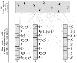
Figure 1: Hash tables and buckets, containing pointers to vectors in memory, in our HashSieve implementa-tion. Example with 9 vectors in the system.

hi(v) = hi(w) if and only if hi,j(v) = hi,j(w) for allj = 1, . . . ,K. For each of theThash tables, we build such a ran-dom, combined hash functionhi, leading to T hash tables

H1, . . . ,HTwith different associated hash functionsh1, . . . , hT. As the range of each of these combined hash functions is

{0,1}K

, the number of hash buckets in each table is 2K . Finally, by increasingKandT, the hash functions become more and more selective and will only map vectors to the same bucket if they are really close to one another in space. However, increasingKandTcomes at the cost of increasing the space complexity; to actually be able to find list vectors in this hash table, we need to store all list vectors in each of the hash tables as well. Also, to find candidate reducing vectors in these hash tables, we need to compute theThash values of the target vectorvand performThash table look-ups. Thus, at some point, making the number of hash tables

Tbigger will not improve the time complexity any more. A detailed analysis reveals the (asymptotic) optimal choices of

KandT. For the angular hash family considered in [12], it was shown thatK = 0.2209n+o(n) and T= 20.1290n+o(n) are asymptotically optimal. Thus, for high dimensions, the choices K = b0.2209ne and T = b20.1290ne (i.e., the lead-ing terms rounded to the nearest integer) seem reasonable. We will refer to these, from now on, as optimal parame-ters, although this is an abuse of notation since they are not necessarily optimal.

3.2

Implementation

In order to implement HashSieve efficiently, many deci-sions have to be made and practical tweaks have to be con-sidered. The original paper already considered some prac-tical improvements to the most general, theoreprac-tical formu-lation of the algorithm, such as using very sparse random hash vectors ai,j to make hash computations significantly

cheaper. Also, since commonly both w and −w are com-pared to v, one can merge the buckets labeled hi(v) and

hi(−v) into one bucket, as done in Line 6 of Algorithm 1. Implementation details do matter for performance, and they must be addressed in our implementation if high per-formance is to be achieved. Buckets can be implemented with linked-lists or vectors which must be re-sized whenever they become full. Figure 1 shows the scheme that we im-plemented. Whenever a vector is to be added to a bucket, we store a pointer to the vector, that is stored sparsely in memory, without any particular organization, so no mem-ory is replicated. Both linked-lists and vectors would have advantages and disadvantages to implement buckets, but as the pointers to vectors are stored within the buckets without any particular order, we chose to implement them as arrays, which are more cache-friendly. The arrays start with a pool of pointers, to avoid several (expensive) singular allocations, and are resized whenever needed.

Another important point with regards to our implemen-tation is that we combine steps (ii) and (iii) together. That is, we reducew with unreduced vectorsv as well, instead of waiting until v is completely reduced. We performed some experiments to find out that our decision is right, performance-wise, because many inner products are saved. Inner products were also vectorized with SSE4.1 and the al-gorithm stops onceccollisions, wherec=α×no_vectors

+β, are generated (in the experimental section, we define bothαandβ). To generate samples, we used Klein’s algo-rithm, as implemented in [15].

4.

A PARALLEL VARIANT OF HASHSIEVE

algorithms on shared-memory architectures [15, 14]. In such a scheme, each thread executes the sequential sieving kernel, i.e., generation of a sample (either from scratch or popped from stack), reduction against existing samples, and storing in memory (e.g. in a global list, as in GaussSieve). How-ever, this results in multiple concurrent memory accesses, which must be handled via some sort of synchronization. In GaussSieve, the concurrency comes down to concurrent in-sertions and removals in a list of vectors, which was solved before with a lock-free, scalable, linked-list list on shared-memory systems [15].

In this section, we analyse the concurrency of a coarse-grained parallel version of HashSieve and we present a prob-able lock-free system that ensures the correctness of that parallel version, while probably executing without actual locks.

Concurrency in parallel HashSieve.

parallelization can be applied to HashSieve as well (each thread would then sample a vector, reduce it against the elements in the hash tables and insert/remove elements ac-cordingly), it becomes considerably more difficult to ensure correctness without resorting to very conservative (and ex-pensive) locking mechanisms. There are two concurrent op-erations in such a scheme. The most obvious is the concur-rent insertion and removal of vectors in each bucket. The other is the concurrent use of multiple vectors throughout the execution, for actual reductions. Since every hash ta-ble has one pointer to every vector in the system, several threads can access (and potentially write) the same vector at the same time, either via the same hash table, or via different hash tables. In short, different threads can access the same buckets and vectors (even if they are working with different hash tables and different buckets).

A (probable) lock-free mechanism.

use of these operations in a parallel execution, we imple-mented a probable lock-free mechanism, i.e., a synchroniza-tion mechanism implemented with locks that will likely act as a lock-free mechanism. This means that locks are only used when strictly required, and chances are that they are never required, because contention is very low. When locks are not strictly required, they are executed as a single, non-blocking CAS operation (i.e. no locking occurs).

To implement this probable lock-free mechanism, we in-troduced a variable per vector and per bucket, which is atomically updated whenever a vector is used (both to read and write). For the buckets, each thread loops until the vari-able is successfully set to “1”, which happens only when the value is originally “0”, as in a spin-lock. This resolves two sources of concurrency: concurrent management of buckets, by different threads, and concurrent accesses to the same vector, by different threads, through the same hash table.

For vectors, that can still be accessed concurrently through different hash tables, each thread tries to set the variable atomically to “1” as well, but in this case the vector is ig-nored if the operation is not successful, and the next vector in line is considered (we refer to this as “a lock”, which never causes thread locking). An illustrative example of this case is the reduction of a samplev against a given set of candi-datesw1,...,wn. If the candidate vectorw1≤k≤n is “locked” (which means that it is either being read or written by an-other thread), the reduction of v against wk will not be

attempted, and the executing thread will continue the pro-cess fromwk+1 onwards. This means that, in this specific iteration,wkwill not be revisited again. The update of these variables is done once the vector is not needed any longer, and no atomic updates are used. This guarantees that the same vector is only accessed by one thread at a time.

There are two caveats that need to be addressed in this process. First and foremost, we refer to our implemen-tation as a relaxed variant of HashSieve, since punctual missed reductions might occur in specific iterations, if dif-ferent threads try to access the same vectors concurrently (one gets “the lock” and the others are not considered), as mentioned before. We believe that this is not too much of a problem because (1) the probability of having different threads accessing the same vectors is very low and (2) the vast majority of vectors is not suitable for the reduction of samples anyway [7, 15, 14]. This is known from the exper-iments with relaxed versions of sieving algorithms, which showed that disregarding vectors at some point does not in-crease the convergence time of the algorithms unless those vectors are ignored from that moment on [15, 17], which is not the case in our implementation. The biggest proof that missing reductions occasionally is not a serious issue, is HashSieve itself, since HashSieve is already a somewhat relaxed version of GaussSieve, as explained in [12].

In HashSieve, however, it must be noted that the proba-bility of vectors to be suitable candidates is higher than in GaussSieve. Thus, our probable lock-free mechanism intro-duces a second level of relaxation. Again, we stress that this relaxation is not problematic, due to the aforementioned rea-sons, which is ultimately proved by our experiments, which delivered the optimal solution with all numbers of threads and in all lattices.

The second important point in our implementation is that, although we implement spin-locks to ensure that only one thread modifies the contents of each bucket at a time, these will, probabilistically speaking, act only as atomic updates of variables (i.e. only the first iteration of the loop is ex-ecuted), thus not causing any actual blocking of threads. This is because the number of buckets per hash table grows exponentially with the dimension of the lattice, according to the optimal values of Tand K(which we used, whenever possible). For instance, we use 212 _{buckets per hash table} for a lattice in dimension 60, whereas that number increases to 218 for a lattice in dimension 90. For a sensible num-ber of threads in shared-memory systems (e.g. <128), the probability of having two or more threads accessing the same bucket is very small (plus, threads do many more operations then accessing buckets).

5.

EXPERIMENTS AND RESULTS

An analysis was carried out with several random lattices, generated with Goldstein-Mayer bases, in multiple dimen-sions, available on theSVP-challenge3 website (all of which of seed 0). Table 1 provides the specifications of the test platform, which runs Ubuntu 11.10, kernel 3.0.0-32-generic. The code was compiled with Intel icpc 13.1.3. We used the-O2 optimization flag, since it was slightly better than-O3. Every experiment was repeated three times and the best sample was chosen, except when said otherwise. The elapsed time of lattice reduction is not included in the

3

#Sockets 2

CPU manufacturer Intel

Model number E5-2670

Launch date Q1’12

Micro-architecture Sandy Bridge

Frequency 2600 MHz

Cores 8

SMT Hyper-threading

L1 Cache 8×32 kB

L2 Cache 8×256 kB

L3 Cache 20 MB shared

System memory 128 GBs

Table 1: Specifications of the test platform. SMT stands for Simultaneous multi-threading.

results. Target norms (i.e., the algorithm stops as soon as it finds a vector whose norm is equal or smaller than the tar-geting norm) were never used, and the norm of the output vector of each and every run (sequential and parallel) was always the same. We used the default stopping criterion, i.e.

α= 0.1 andβ= 200, and we used version 5.5.2 of NTL4.

5.1

Sequential implementation

In this section, we present several results pertaining to the performance of our implementation of HashSieve running in sequential, i.e. our parallel implementation running with one thread. In particular, we show the results of the following experiments:

• Quantification of the overhead of the (probable) lock-free mechanism we implemented, necessary for the cor-rectness of our parallel variant of HashSieve, and com-parison with an implementation of GaussSieve;

• Comparison of HashSieve and GaussSieve with respect to convergence rate, in terms of used vectors. Devel-opment of a memory usage model that captures the majority of the memory usage of our implementation.

For these trials, we reduced the input lattices with NTL’s BKZ, running with windowβ= 20, we set thedparameter in Klein’s algorithm to log(n)/20 (a smaller value leads to incorrect results for lattices in dimensions<70, as discussed in Section 4.4 of [15]), and our pool of vectors per bucket starts with 20 vectors, increasing by 20 vectors whenever it is seen full. We also vectorized the inner product kernel and the kernel which adds one vector to another, with SSE 4.1. The coordinates of the vectors are stored as shorts, thereby permitting us to store 8 coordinates per SSE register.

5.1.1

Overhead of (probable) lock-free mechanism

and comparison with GaussSieve

In this subsection, we compare the efficiency of our im-plementation with the probable lock-free system turned on and off (for which we used compiler pragmas), with the lock-free GaussSieve implementation presented in [15], all of which running with one thread (otherwise the implemen-tation would have data races with the lock-free mechanism turned off).

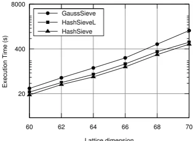
Our results confirm that HashSieve outperforms GaussSieve not only in theory but also in practice. As Figure 2 shows, HashSieve outperforms GaussSieve for every tested dimen-sion, in a single-threaded application, with a speedup fac-tor of up to ≈2.2x with the lock-free mechanism turned 4

http://www.shoup.net/ntl/

20 400 8000

60 62 64 66 68 70

Lattice dimension GaussSieve

HashSieveL HashSieve

E

xe

cutio

n

Tim

e

(s)

Figure 2: Execution time, in seconds, for HashSieve with (HashSieveL) and without the probable lock-free system (HashSieve), and GaussSieve (1 thread), on lattices in dimensions 60-70 (less is better).

on and a factor of up to ≈2.5x with the lock-free mecha-nism turned off. According to the theoretical complexity bounds, the speedups are expected to increase with the di-mension, but it is impractical to test higher dimensions with a single thread and, therefore, confirm this in practice for a single thread (Section 5.2.2 shows such results for parallel executions). The (probable) lock-free system incurs about 20% overhead, compared to the single-threaded execution of HashSieve. However, it should be noticed that for parallel executions, some computations will likely be discarded due to the relaxation of the algorithm, thereby amortizing this overhead. For these trials, we used the optimal values of

K, T and BUCKETS, as shown in Table 2, since no memory restrictions were encountered.

5.1.2

HS vs GS: convergence rate and memory

In the following, we show results pertaining to the con-vergence rate of GaussSieve and HashSieve, in terms of used vectors. Figure 3 shows the number of vectors used by the sequential versions of HashSieve and GaussSieve, for lattices in dimensions 40-70, in steps of 2, when executed with one thread (both parallel versions relax the properties of the algorithms, thereby possibly changing the number of vec-tors used to converge). Since the probable lock-free mecha-nism we implemented for HashSieve does not interfere with the work-flow of the algorithm when executing with a sin-gle thread (other than introducing the overhead shown in Section 5.1.1), our HashSieve implementation uses the same number of vectors both when the probable lock-free mecha-nism is turned on and off.

We conclude that, as expected in [12], HashSieve uses more vectors to converge than GaussSieve, for lattices up to dimension 70. In particular, the number of vectors in

Dimension 60 62 64 66 68 70

K 13 14 14 15 15 15

T 214 256 306 366 437 523

BUCKETS 212 213 213 214 214 214

102 103 104 105 106

40 42 44 46 48 50 52 54 56 58 60 62 64 66 68 70

Lattice dimension HashSieve

GaussSieve

N

um

be

r o

f vector

s

Figure 3: Number of vectors for convergence of

HashSieve and GaussSieve (1 thread), for lattices in dimensions 40-70.

HashSieve grows roughly according to 2(0.21n+1.95), a func-tion we obtained by curve fitting, for lattices in dimensions 40-70, in steps of 2. The relative difference between the al-gorithms seem to decrease with the lattice dimension of the lattice, but it is impractical to test higher dimensions with a single thread and therefore no assumptions can be made for bigger dimensions.

The number of vectors that HashSieve uses is closely re-lated to a critical factor of the algorithm: the amount of used memory. GaussSieve samples vectors and reduces them against one another, storing them in a big list that grows over time. HashSieve uses vectors likewise, storing them in memory without any particular organization, but makes also use of many hash tables of pointers to those vectors, which increases memory consumption. For big dimensions, this becomes a problem, since even 128 GB of RAM are easily exceeded. In order to estimate beforehand what parameters can be used for each execution without exceeding the avail-able memory, we devised the following memory usage model of our HashSieve implementation:

mHS=T∗BUCKETS∗(16 + 20∗8)

| {z }

HashTables

+ 2∗T∗K∗2

| {z }

A

bytes.

The first term on the right hand side, labeled HashTables, is given by the data structure that holds the buckets:bucket HashTables[T][BUCKETS]. Each bucket is a structure in the following form:

struct bucket{

Vector** vectors; (pool starts with 20 pointers) unsigned int length;

unsigned int size; }

i.e., 8 bytes forlengthandsize(4 bytes each) and 8 bytes for the pointervectors(the word size on the test system is 64 bits), which starts off with a pool of 20 pointers (i.e., 20

×8 = 160 bytes) to structs of the type vector. Each of these structures has the following form:

struct vector{ USED_TYPE data[N];

unsigned long norm; struct vector *next; char lock;

}

whereUSED_TYPEcan either be intorshort. We use the latter, which is implemented in Unix systems with 2 bytes, since we can make better use of the SSE registers. The pointer to an element of the same type is used for the stack. The second part of the equation is given by the data struc-ture that represents the Hash matrices: unsigned short A[T][K][2].

This model accounts for the memory that the implementa-tion allocates at launch time, i.e. right before the reducimplementa-tion of the basis. In order to estimate the memory that is used throughout the execution, there are other factors that must be taken into account. There are essentially two other rele-vant contributions to the total memory of the application.

The first is the memory that is used to store vectors. We extrapolate that the number of vectors is governed by the functionv(n) = 2(0.21n+1.95)_{, as mentioned before. Although} we noticed that the number of used vectors in the parallel version is different from the the sequential version, we be-lieve that the function of the sequential version offers reason-able estimates of the number of used vectors in the parallel version. The size of each vector is 2n+ 17 bytes, where n

is the dimension of the lattice and we use shorts for each coordinate.

The second is the memory used to extend the arrays that represent the buckets. While we can provide a good estimate for the former, it is not trivial to provide such estimate for the latter. In our implementation, we extend each bucket in 20 positions whenever they become full. What can be calculated is the average and worst case scenarios of memory used by the buckets. However, our model is intended to determine whether a set of parameters is feasible, and so it does not account for bucket extensions.

The probable lock-free system that we implemented in-creases the memory usage of our implementation as well, with a 1-byte (char) lock per bucket and per hash table, and a 1-byte (char) lock per vector. In particular, we allo-cate a matrixchar LocksForHashTables[T][BUCKETS], and a char per vector. Therefore, the final memory usage model we arrived at, for our parallel implementation of HashSieve is the following:

mHSL=mHS+ T∗BUCKETS

| {z }

LocksForHashTables

+ v

|{z}

no. vectors

∗(2n+17)bytes.

Apart from these data-structures and vectors that are cre-ated throughout the execution of the application, there are additional data-structures, all of which have lower order contribution to the memory usage of the implementation. Padding can also be used to ensure that the addresses of the data structures are multiples of the word size, which might increase the memory spent with each vector. For instance, a vector in dimension 80 occupies 177 bytes, which would be augmented to 192 bytes. However, we expect that our model is accurate enough to predict whether the memory used by our implementation exceeds the available memory in the system or not, especially for high lattice dimensions, which are more interesting to test.

to capture the Resident Set Size (RSS), i.e. the amount of process’s memory that is held in RAM, of our application. To this end, we invoke the (ps -x pid)system call after the execution of the parallel region but before the applica-tion terminates. The RSS captures the memory spent by the whole application, which includes memory spent by the libraries that are used in the implementation (e.g. NTL for lattice reduction with BKZ and OpenMP for creating and managing the parallel region), which is not predicted by our model.

0.01 0.1 1 10 100

40 42 44 46 48 50 52 54 56 58 60 62 64 66 68 70

Lattice dimension RSS

Model Diff(%)

103

104

105

106

107

D

ata siz

e (

kB

)

Figure 4: Data size, in kB, stored in RAM. Resident Set Size (RSS), prediction of our model. The grayed out area concerns the difference between the actual RSS and our model, in percentual points.

As Figure 4 shows, our model gets very close to the actual RSS of our implementation for big lattice dimensions. This is due to the fact that, although our model only accounts for the main (i.e., bigger) data structures in the implementation, they grow exponentially in size with the lattice dimension, and so the remaining data structures become negligible. In particular, Figure 4 shows that for lattices bigger than di-mension 58, the difference between the actual RSS and our model is always lower than 20%, and most of the times very close to 10%.

Our model shows that, by choosing the optimal param-eters of T, Kand BUCKETS, the 128 GB of our machine are only enough to test lattices up to dimension 86, wherein the application spends around 100 GB of RAM (whereT,Kand

BUCKETS are assigned 19, 2189 and 218, respectively). Ac-cording to our model, executing a lattice in dimension 100 with optimal parameters would require over 2.5 TB of RAM. Due to the memory restriction of our test machine, we will use, from here on, the parametersT,Kand BUCKETSas 19, 2189 and 218_{, respectively, for lattices in dimensions≥86.}

5.2

Parallel implementation

5.2.1

Scalability

This section records the trials that we conducted to quan-tify the scalability of our implementation on our test plat-form, for random lattices in dimensions 60, 64, 70, 74 and 80. Lower dimensions are either solved very quickly or the lattice reduction process finds the shortest vector per se, rendering a scalability analysis worthless. Running the im-plementation for higher dimensions, on the other hand, is

impractical for a single thread. We were still able to use the optimal parameters of HashSieve in these dimensions, which are shown in Tables 2 and 4. We BKZ-reduced the lattices up to dimension 70 withβ= 20, and higher dimensions with

β= 30.

As in [15], the time spent within the sampling routine increases for lower values of Klein’s algorithm parameterd, which lowers the scalability of the implementation because the sampler routine does not scale well. For that reason, and to properly assess the scalability of our implementation, we set the Klein’s algorithm parameterdto 20 for every lattice.

1 10 100

1 2 4 8 16 32

#Threads

Dim 80 Dim 74 Dim 70 Dim 64 Dim 60 103

104

105

106

E

xe

cutio

n

Tim

e

(s)

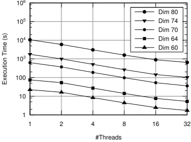
Figure 5: Execution time, in seconds, for HashSieve with 1-32 threads, on lattices in dimensions 60-80 (less is better).

Figure 5 shows the execution time of our implementation, for 1-32 threads. The application scales well for up to 32 threads, for various lattices between dimensions 60 and 80. Unfortunately, scalability experiments are impractical for higher lattices, since every and each thread set-up is exe-cuted three times (e.g., solving a lattice in dimension 84 with 1 thread would take about 38 hours). As shown in Ta-ble 3, the speedup of our implementation increases, in gen-eral, with the dimension, because the higher the dimension, the more time is spent on reducing each sample, rather than on generating more samples. In some cases, our implemen-tation achieves efficiency levels of almost 90%. We believe that the integration of a very scalable sampler in our im-plementation would increase its scalability. This could also be achieved with higher values for Klein’s parameterd(e.g., log(n)), as mentioned above, but lower values forddecrease the overall performance of the algorithm, because larger vec-tors are sampled and the algorithm converges faster when fed with shorter algorithms.

5.2.2

Comparison with GaussSieve

Dimension 60 Dimension 64 Dimension 70 Dimension 74 Dimension 80

Cores S E S E S E S E S E

2 1.37x 69% 1.40x 70% 1.69x 84% 1.76x 88% 1.77x 89%

4 2.66x 67% 2.75x 69% 3.33x 83% 3.43x 86% 3.45x 86%

8 5.07x 63% 5.27x 66% 6.42x 80% 6.64x 83% 6.56x 82%

16 9.05x 57% 9.80x 61% 11.83x 74% 12.16x 76% 11.76x 74% 32 13.01x 41% 14.08x 44% 17.48x 55% 17.14x 54% 16.26x 51%

Table 3: Speedups (S) and Efficiency (E) of our HashSieve implementation running on five random lattices (dimensions 60, 64, 70, 74 and 80). SMT is used in grayed out rows.

will only get bigger with increasing dimensions, unless sub-optimal parameters are used.

Dim 66 68 70 72 74 76 78

K 15 15 15 16 16 17 17

T 366 437 523 625 748 894 1069

BUCKETS 214 ₂14 ₂14 ₂15 ₂15 ₂16 ₂16

BKZ-β 20 20 20 30 30 30 30

mHSL 1.00 1.19 1.43 3.40 4.06 9.70 11.60

Table 4: HashSieve parameters used for K, T and

BUCKETS, BKZ-β and memory model prediction

(in GB) for various lattices in dimensions 66-78.

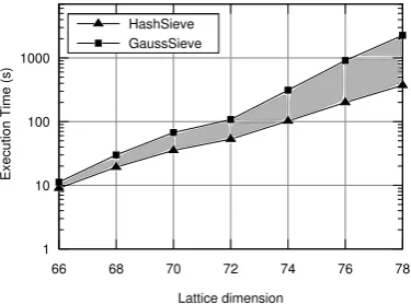
Figure 6 shows the execution time of our implementation and the GaussSieve implementation presented in [15], both running with 32 threads. HashSieve outperforms GaussSieve, as verified with the sequential versions, and the difference between both algorithms grows with the lattice dimension.

1 10 100 1000

66 68 70 72 74 76 78

Lattice dimension HashSieve

GaussSieve

E

xe

cutio

n

Tim

e

(s)

Figure 6: Execution time, in seconds, for HashSieve and GaussSieve, with 32 threads, on lattices in di-mensions 66-78 (less is better).

5.2.3

Practicability experiments

In this section, we report the results of our experiments on the practicability of our parallel HashSieve implementation on lattices in large dimensions. We report the largest lat-tice dimensions that we were able to find and the execution time that our implementation took. The main limitation we encountered during the trials we conducted was the lack of RAM to use the optimal parameters of HashSieve.

Since the machine we used has 128 GB of RAM, our ex-periments were limited to K = 18, T = 1828 and BUCKETS

= 131072, i.e., far from being the optimal parameters. Un-fortunately, the optimal parameters are impractical for ma-chines that are not equipped with unusual amounts of RAM. For instance, the optimal parameters for dimension 96, (K= 21,T= 5345 andBUCKETS= 220_{) would require almost 1 TB} of RAM only for the data structures that are allocated at launch time. Therefore, we expect that better parameters would result in a much better execution time of our imple-mentation. Yet, we were able to solve the SVP on several lattices, from dimension 86 to dimension 96, all in less than 24h, as Table 5 shows.

Dim 86 88 90 92 94 96

Time (h) 1.92 2.38 3.43 7.35 11.07 17.38

Table 5: Execution time of our parallel implemen-tation of HashSieve running with 32 threads on the test platform, in hours.

For these experiments, we used BKZ-β= 34, and Klein’s parameter = 70 (which is expected to be the best for di-mensions higher than 80, even if poor scalability is achieved - a claim that is too time consuming to be verified). Each execution was run only once.

6.

CONCLUSIONS AND OUTLOOK

This paper presents a parallel implementation of Hash-Sieve, a recently proposed sieving algorithm to solve the SVP on lattices. Our implementation scales considerably well on a 16-core system with SMT, and outperforms the most efficient shared-memory GaussSieve implementation, published in [15]. Therefore, we were able to verify in prac-tice the results that were expected from theory.

In parallel, HashSieve has more concurrent operations than GaussSieve. Our implementation uses a probable lock-free algorithm, which might cause missed reductions, but chances are that, for sufficiently large numbers of hash tables and buckets, no locks are used (or, in other words, no threads block). With our implementation, we are able to solve the SVP on an arbitrary lattice in dimension 96 in less than 17.5 hours, with our 16-core test machine.

fit of the execution times of our implementation for lattices between 80 and 96 (all of which with BKZ-β= 34, Klein’s parameter d = 70), in seconds, lies between 2(0.32n−15) _or 2(0.33n−16). This means that, if we disregard memory usage and loss of efficiency when using larger numbers of cores, we would solve the SVP in dimension 120 in less than 2 days, with 100 machines identical to our benchmarking machine.

The main drawback of HashSieve is the amount of used memory. In fact, this limited our expectation of determin-ing how practical HashSieve is for high dimensional lattices with optimal parameters, since our system limited our ex-periments to 128 GB. With more RAM, one would be able to determine if HashSieve can outperform enumeration al-gorithms with extreme pruning. Depending on this answer, which we plan to assess in future work, it might be prefer-able to invest money on systems with very large memories rather than high core counts, if the SVP on high dimensional lattices is to be solved.

The results we achieved with the proposed parallel imple-mentation of HashSieve are, in our view, very promising. However, due to the inherent characteristics of the algo-rithm, our implementation is not as scalable as GaussSieve, and there is an array of subjects which affect the perfor-mance of HashSieve, that we will study in the near future:

• Impact of different samplers on our implementation;

• Different bucket organizations (e.g. vectors by increas-ing norm, as done in GaussSieve, for list L);

• Implementation of probing (cf. [12]), to reduce mem-ory usage.

7.

ACKNOWLEDGMENTS

This work has been co-funded by the DFG as part of project P1 within the CRC 1119 CROSSING. The project did also fund a visit from Thijs Laarhoven to Darmstadt, from Nov. 10th_{till Nov. 14}th_{2014. The authors thank also} Cristiano Sousa for revising the lock-free mechanism and Shahar Timnat for revising the manuscript.

8.

REFERENCES

[1] Erik Agrell, Thomas Eriksson, Alexander Vardy, and Kenneth Zeger. Closest point search in lattices.IEEE Transactions on Information Theory, 48(8):2201–2214, 2002.

[2] Mikl´os Ajtai. The shortest vector problem inL2 is NP-hard for randomized reductions (extended abstract). InSTOC, pages 10–19, 1998.

[3] Mikl´os Ajtai, Ravi Kumar, and D. Sivakumar. A sieve algorithm for the shortest lattice vector problem. In

STOC, pages 601–610, 2001.

[4] Anja Becker, Nicolas Gama, and Antoine Joux. A sieve algorithm based on overlattices. InANTS, pages 49–70, 2014.

[5] Joppe Bos, Michael Naehrig, and Joop van de Pol. Sieving for shortest vectors in ideal lattices: a practical perspective. Cryptology ePrint Archive, Report 2014/880, 2014.

[6] Moses S. Charikar. Similarity estimation techniques from rounding algorithms. InSTOC, pages 380–388, 2002.

[7] Robert Fitzpatrick, Christian Bischof, Johannes Buchmann, ¨Ozg¨ur Dagdelen, Florian G¨opfert, Artur Mariano, and Bo-Yin Yang. Tuning GaussSieve for speed. InLATINCRYPT, pages 284–301, 2014. [8] Nicolas Gama, Phong Nguyen, and Oded Regev.

Lattice enumeration using extreme pruning. In

EUROCRYPT, pages 257–278, 2010.

[9] Craig Gentry. Fully homomorphic encryption using ideal lattices. InSTOC, pages 169–178, 2009. [10] Guillaume Hanrot, Xavier Pujol, and Damien Stehl´e.

Algorithms for the shortest and closest lattice vector problems. InIWCC, pages 159–190, 2011.

[11] Tsukasa Ishiguro, Shinsaku Kiyomoto, Yutaka Miyake, and Tsuyoshi Takagi. Parallel Gauss Sieve algorithm: Solving the SVP challenge over a 128-dimensional ideal lattice. InPKC’14, pages 411–428, 2014. [12] Thijs Laarhoven. Sieving for shortest vectors in

lattices using angular locality-sensitive hashing. Cryptology ePrint Archive, Report 2014/744, 2014. [13] Thijs Laarhoven, Joop van de Pol, and Benne

de Weger. Solving hard lattice problems and the security of lattice-based cryptosystems. Cryptology ePrint Archive, Report 2012/533, 2012.

[14] Artur Mariano, ¨Ozg¨ur Dagdelen, and Christian Bischof. A comprehensive empirical comparison of parallel ListSieve and GaussSieve. InAPCI&E, 2014. [15] Artur Mariano, Shahar Timnat, and Christian

Bischof. Lock-free GaussSieve for linear speedups in parallel high performance SVP calculation.

SBAC-PAD’14, 2014.

[16] Daniele Micciancio and Panagiotis Voulgaris. Faster exponential time algorithms for the shortest vector problem. InSODA, pages 1468–1480, 2010. [17] Benjamin Milde and Michael Schneider. A parallel

implementation of GaussSieve for the shortest vector problem in lattices. InPaCT, pages 452–458, 2011. [18] Phong Q. Nguyen and Thomas Vidick. Sieve

algorithms for the shortest vector problem are practical.Journal of Mathematical Cryptology, 2(2):181–207, 2008.

[19] Xavier Pujol and Damien Stehl´e. Solving the shortest lattice vector problem in time 22.465n. Cryptology ePrint Archive, Report 2009/605, 2009.

[20] Michael Schneider. Sieving for short vectors in ideal lattices. InAFRICACRYPT, pages 375–391, 2013. [21] Michael Schneider and Norman G¨ottert. Random

sampling for short lattice vectors on graphics cards. In

CHES, pages 160–175, 2011.

[22] Claus-Peter Schnorr and Martin Euchner. Lattice basis reduction: Improved practical algorithms and solving subset sum problems.Mathematical Programming, 66(2–3):181–199, 1994.

[23] Xiaoyun Wang, Mingjie Liu, Chengliang Tian, and Jingguo Bi. Improved Nguyen-Vidick heuristic sieve algorithm for shortest vector problem. InASIACCS, pages 1–9, 2011.