LWE Without Modular Reduction and
Improved Side-Channel Attacks Against BLISS
Jonathan Bootle1, Claire Delaplace2,3, Thomas Espitau4, Pierre-Alain Fouque2, and Mehdi Tibouchi5
1
University College London
2
Univ Rennes
{claire.delaplace,pierre-alain.fouque}@univ-rennes1.fr
3
Univ Lille 4
Sorbonne Universit´e
5
NTT Secure Platform Laboratories
Abstract. This paper is devoted to analyzing the variant of Regev’s learning with errors (LWE) problem in which modular reduction is omitted: namely, the problem (ILWE) of recovering a vectors ∈ Zn given polynomially many samples of the form(a,ha,si+e) ∈Zn+1whereaandefollow fixed distributions. Unsurprisingly, this problem is much easier than LWE: under mild conditions on the distributions, we show that the problem can be solved efficiently as long as the variance ofeis not superpolynomially larger than that ofa. We also provide almost tight bounds on the number of samples needed to recovers.
Our interest in studying this problem stems from the side-channel attack against the BLISS lattice-based signature scheme described by Espitau et al. at CCS 2017. The attack targets aquadraticfunction of the secret that leaks in the rejection sampling step of BLISS. The same part of the algorithm also suffers from alinearleakage, but the authors claimed that this leakage could not be exploited due to signature compression: the linear system arising from it turns out to benoisy, and hence key recovery amounts to solving a high-dimensional problem analogous to LWE, which seemed infeasible. However, this noisy linear algebra problem does not involve any modular reduction: it is essentially an instance of ILWE, and can therefore be solved efficiently using our techniques. This allows us to obtain an improved side-channel attack on BLISS, which applies to 100% of secret keys (as opposed to≈7%in the CCS paper), and is also considerably faster.
Keywords:LWE problem, lattice-based cryptography, side-channel analysis, BLISS, least squares regression, sta-tistical learning, compressed sensing, concentration inequalities.
1
Introduction
Learning with errors. Regev’slearning with errorsproblem (LWE) is the problem of recovering a uniformly random vectors∈(Z/qZ)ngiven polynomially many samples of the form(a,ha,si+emodq), withauniform in(Z/qZ)n, andesampled according to a fixed distribution overZ/qZ(typically a discrete Gaussian). Regev showed [1] that for suitable parameters, this problem is as hard as worst-case lattice problems, and is polynomial-time equivalent to its decision version, which asks to distinguish the distribution of tuples(a,ha,si+emodq)as above from the uniform distribution over(Z/qZ)n+1. These results are a cornerstone of modern lattice-based cryptography, which is to a large extent based on LWE and related problems.
2
in which the scalar productha,siis partly hidden not by adding some noisee, but by disclosing only its most significant bits.
Recently, further exotic variants have emerged in association with schemes submitted to the NIST postquantum cryptography standardization process. One can mention for example Compact-LWE [22,23], which has been bro-ken [24,25,26]; learning with truncation, considered in pqNTRUSign [27]; and Mersenne variants of Ring-LWE, introduced for ThreeBears [28] and Mersenne–756839 [29].
The ILWE problem. In this paper, we introduce a simpler variant of LWE in which computations are carried out over Zrather thanZ/qZ, i.e. without modular reduction. More precisely, we consider the problem which we call ILWE (“integer LWE”) of finding a vectors∈ Zngiven polynomially many samples of the form(a,ha,si+e)∈ Zn+1, whereaandefollow fixed distributions onZ.
This problem may occur more naturally in statistical learning theory or numerical analysis than it does in cryptog-raphy; indeed, contrary to LWE, it is usually not hard. It can even be solved efficiently when the erroreismuch larger than the inner productha,si(but not superpolynomially larger), under relatively mild conditions on the distributions involved.
The fact that standard learning techniques like least squares regression should apply to this problem can be regarded as folklore, and is occasionally mentioned in special cases in the cryptographic literature (see e.g. [10,§7.6]). The main purpose of this work is to give a completely rigorous treatment of this question, and in particular to analyze the number of samples needed to solve ILWE both in an information-theoretic sense and using concrete algorithms.
ILWE and side-channel attacks on BLISS. Our main motivation for studying the ILWE problem is a side-channel attack against the BLISS lattice-based signature scheme described by Espitau et al. at CCS 2017 [30].
BLISS [31] is one of the most prominent, efficient and widely implemented lattice-based signature schemes, and it has received significant attention in terms of side-channel analysis. Several papers [32,33,30] have pointed out that, in available implementations, certain parts of the signing algorithm can leak sensitive information about the secret key via various side-channels like cache timing, electromagnetic emanations and secret-dependent branches. They have shown that this leakage can be exploited for key recovery.
We are in particular interested in the leakage that occurs in the rejection sampling step of BLISS signature gen-eration. Rejection sampling is an essential element of the construction of BLISS and other lattice-based signatures following Lyubashevsky’s “Fiat–Shamir with aborts” framework [34]. Implementing it efficiently in a scheme using Gaussian distributions, as is the case for BLISS, is not an easy task, however, and as observed by Espitau et al., the optimization used in BLISS turns out to leak two functions of the secret key via side-channels: anexact,quadratic function, as well as anoisy,linearfunction.
The attack proposed by Espitau et al. relies only on the quadratic leakage, and as a result uses very complex and computationally costly techniques from algorithmic number theory (a generalization of the Howgrave-Graham–Szydlo algorithm for solving norm equations). In particular, not only does the main, polynomial-time part of their algorithm takes over a CPU month for standard BLISS parameters, technical reasons related to the hardness of factoring make their attack only applicable to a small fraction of BLISS secret key (around7%; these are keys satisfying a certain smoothness condition). They note that using thelinearleakage instead would be much simpler if the linear function was exactly known, but cannot be done due to its noisy nature: recovering the key then become a high-dimensional noisy linear algebra problem analogous to LWE, which should therefore be hard.
However, the authors missed an important difference between that linear algebra problem and LWE: the absence of modular reduction. The problem can essentially be seen as an instance of ILWE instead, and our analysis thus shows that it is easy to solve. This results in a much more computationally efficient attack taking advantage of the leakage in BLISS rejection sampling, which moreover applies toallsecret keys.
3 On the theoretical side, our first contribution is to prove that, in an information-theoretic sense, solving the ILWE problem requires at least m = Ω (σe/σa)
2
samples from the ILWE distribution when the error e has standard deviationσe, and the coefficients of the vectorsain samples have standard deviationσa. We show this by estimating the statistical distance between the distributions arising from two distinct secret vectorssands0. In particular, the ILWE problem is hard whenσeis superpolynomially larger thanσa, but can be easy otherwise, including whenσe exceedsσaby a large polynomial factor.
We then provide and analyze concrete algorithms for solving the problem in that case. Our main focus is least squares regression followed by rounding. Roughly speaking, we show that this approach solves the ILWE problem withmsamples when m ≥ C· σe/σa)2lognfor some constantC (and is also a constant factor larger thann, to ensure that the noise-free version of the corresponding linear algebra problem has a unique solution, and that the covariance matrix of the vectorsais well-controlled). Our result applies to a very large class of distributions foraand eincluding bounded distributions and discrete Gaussians. It relies on subgaussian concentration inequalities.
Interestingly, ILWE can be interpreted as a bounded distance decoding problem in a certain lattice inZn(which is very far from random), and the least squares approach coincides with Babai’s rounding algorithm for the approximate closest vector problem (CVP) when seen through that lens. As a side contribution, we also show that even with a much stronger CVP algorithm (including an exact CVP oracle), one cannot improve the number of samples necessary to recoversby more than a constant factor. And on another side note, we also consider alternate algorithms to least squares when very few samples are available (so that the underlying linear algebra system is not even full-rank), but the secret vector is known to be sparse. In that case, compressed sensing techniques using linear programming [35] can solve the problem efficiently.
After this theoretical analysis, we concretely examine the noisy linear algebra problem arising from the linear part of the BLISS rejection sampling leakage, and show that is strongly resembles an ILWE problem, which allows us to estimate the number of side-channel traces needed to recover the secret key.
Simulation results both for the vanilla ILWE problem and the BLISS attack are consistent with the theoretical predictions (only with better constants). In particular, we obtain a much more efficient attack on BLISS than the one in [30], which moreover applies to100%of possible secret keys. The only drawback is that our attack requires a larger number of traces (around20000compared to512in [30] for BLISS–I parameters), and even that is to a large extent counterbalanced by the fact that we can easily handle errors in the values read off from side-channel traces, whereas Espitau et al. need all their leakage values to be exact.
2
Preliminaries
2.1 Notation
Forr ∈ R, we denote bydrc the nearest integer to r (rounding down for half-integers), and by brcthe largest integer less or equal tor. For a vector x = (x1, . . . , xn) ∈ Rn, the p-normkxkp ofx,p ∈ [1,∞), is given by kxkp = |x1|p+· · ·+|xn|p
1/p
, and the infinity norm bykxk∞ = max |x1|, . . . ,|xn|. For a matrixA∈Rm×n, the operator normkAkopp ofAwith respect to thep-norm,p∈[1,∞], is given by:
kAkop
p = sup x∈Rn\{0}
kAxkp kxkp
= sup
kxkp=1
kAxkp.
For any random variableX, we denote byE[X]its expectation and byVar(X) = E[X2]−E[X]2its variance. We writeX ∼χto denote thatXfollows the distributionχ. Ifχis a discrete distribution over some setS, then for any s∈S, we denote byχ(s)the probability that a sample fromχis equal tos. In particular, iff:S→Ris any function andX ∼χ, we have:
E[f(s)] =
X
s∈S
f(s)·χ(s).
Similarly, the statistical distance∆(χ, χ0)of two distributionsχ, χ0over the setSis: ∆(χ, χ0) =1
2
X
s∈S
4
Letρ(x) = exp(−πx2)for allx∈
R. We defineρc,σ(x) = ρ (x−c)/σ
the Gaussian function of parametersc, σ. For any subsetS ⊂Rsuch that the sum converges, we let:
ρc,σ(S) =
X
s∈S
ρc,σ(s).
The discrete Gaussian distributionDc,σcentered atcand of parameterσis the distribution onZdefined by
Dc,σ(x) =
ρc,σ(x) ρc,σ(Z)
= exp −π(x−c)
2/σ2
ρc,σ(Z)
for allx∈Z. We omit the subscriptcinρc,σandDc,σwhenc= 0.
2.2 LWE over the Integers
It is possible to define a variant of the LWE problem “over the integers”, i.e. without modular reduction. We call this problem ILWE(“integer-LWE”), and define it as follows. The problem arising from the scalar product leakage in the BLISS rejection sampling is essentially of that form.
Definition 2.1 (ILWE Distribution).For any vectors∈Znand any two probability distributionsχa, χeoverZ, the ILWE distributionDs,χa,χe associated with those parameters (which we will simply denoteDsfor short whenχa, χe
are clear) is the probability distribution overZn×Zdefined as follows: samples fromDs,χa,χeare of the form
(a, b) = a,ha,si+e
with a←χna ande←χe.
Definition 2.2 (ILWE Problem).TheILWE problemis the computational problem parametrized byn, m, χa, χein which, givenmsamples{(ai, bi)}1≤i≤mfrom a distribution of the formDs,χa,χe for somes∈ Z
n, one is asked to recover the vectors.
2.3 Subgaussian Probability Distributions
In this paper, the distributionsχa,χe we will consider will usually be of mean zero and rapidly decreasing. More precisely, we will assume that those distributions aresubgaussian. The notion of a subgaussian distribution was intro-duced by Kahane in [36], and can be defined as follows.
Definition 2.3. A random variableXoverRis said to beτ-subgaussianfor someτ >0if the following bound holds for alls∈R:
Eexp(sX)≤exp
τ2s2
2
. (2.1)
Aτ-subgaussian probability distribution is defined in the same way.
This section collects useful facts about subgaussian random variables; most of them are well-known, and presented mostly in the interest of a self-contained and consistent presentation (as definitions of related notions tend to vary slightly from one reference to the next).
For a subgaussian random variableX, there is a minimalτ such thatX isτ-subgaussian. Thisτ is sometimes called thesubgaussian momentof the random variable (or of its distribution).
As expressed in the next lemma, subgaussian distributions always have mean zero, and their variance is bounded byτ2.
Lemma 2.4. Aτ-subgaussian random variableXsatisfies:
5 Proof. Forsaround zero, we have:
E[exp(sX)] = 1 +sE[X] + s2
2E[X
2] +o(s2).
Since, on the other hand,exp(s2τ2/2) = 1 +s2 2τ
2+o(s2), the result follows immediately from (2.1). ut Many usual distributions overZ or Rare subgaussian. This is in particular the case for Gaussian and discrete Gaussian distributions, as well as allboundedprobability distributions with mean zero.
Lemma 2.5. The following distributions are subgaussian.
(i) The centered normal distributionN(0, σ2)isσ-subgaussian.
(ii) The centered discrete Gaussian distributionDσof parameterσis √σ2π-subgaussian for allσ≥0.283. (iii) The uniform distributionUαover the integer interval[−α, α]∩Zis√α2-subgaussian forα≥3.
(iv) More generally, any distribution over Rof mean zero and supported over a bounded interval[a, b]is b−2a
-subgaussian.
Moreover, in the cases(i)–(iii)above, the quotientτ≥1between the subgaussian moment and the standard deviation satisfies:
(i) τ = 1;
(ii) τ <√2assumingσ≥1.85; (iii) τ ≤p
3/2
respectively.
Proof. See AppendixA.1. ut
The main property of subgaussian distributions is that they satisfy a very strong tail bound. Lemma 2.6. LetX be aτ-subgaussian distribution. For allt >0, we have
Pr[X > t]≤exp− t 2
2τ2
. (2.2)
Proof. Fixt >0. For alls∈Rwe have, by Markov’s inequality:
Pr[X > t] = Pr[exp(sX)> est]≤E[exp(sX)] est
since the exponential is positive. Using the fact thatXisτ-subgaussian, we get:
Pr[X > t]≤exps
2τ2
2 −st
and the right-hand side is minimal fors=t/τ2, which exactly gives (2.2). ut The following result states that a linear combination ofindependentsubgaussian random variables is again sub-gaussian.
Lemma 2.7. LetX1, . . . , Xnbe independent random variables such thatXiisτi-subgaussian. For allµ1, . . . , µn∈
6
Proof. Since theXi’s are independent, we have, for alls∈R:
E[exp(sX)] =E
h
exp s(µ1X1+· · ·+µnXn)
i
=Ehexp(µ1sX1)· · ·exp(µnsXn)
i
=
n
Y
i=1
Eexp(µisXi)
.
Now, sinceXiisτi-subgaussian, we have
Eexp(µisXi)
≤exps
2(µ iτi)2
2
for alli. Therefore:
E[exp(sX)]≤
n
Y
i=1
exps
2(µ iτi)2
2
= exps
2τ2
2
withτ2=µ21τ12+· · ·+µ2nτn2as required. ut
The previous result shows that the notion of a subgaussian random variable has a natural extension to higher dimensions.
Definition 2.8. A random vectorxinRn is called a τ-subgaussian random vector if for all vectorsu ∈ Rn with kuk2= 1, the inner producthu,xiis aτ-subgaussian random variable.
It clearly follows from Lemma 2.7that if X1, . . . , Xn are independent τ-subgaussian random variables, then the random vectorx= (X1, . . . , Xn)isτ-subgaussian. In particular, ifχis aτ-subgaussian distribution, then a random vectorx ∼ χn isτ-subgaussian. A nice feature of subgaussian random vectors is that the image of such a random vector under any linear transformation is again subgaussian.
Lemma 2.9. Letxbe aτ-subgaussian random vector inRn, andA ∈ Rm×n. Then the random vectory =Axis τ0-subgaussian, withτ0 =kATkop
2 ·τ.
Proof. Fix a unit vectoru0∈Rm. We want to show that the random variablehu0,yiisτ0-subgaussian. To do so, first observe that:
hu0,yi=hATu0,xi=µhu,xi whereµ = kATu0k
2, andu = µ1ATu0is a unit vector ofRn. Sincexisτ-subgaussian, we know that the inner producthu,xiis aτ-subgaussian random variable. As a result, by Lemma2.7in the trivial case of a single variable, we obtain thathu0,yi =µhu,xiis |µ|τ
-subgaussian. But by definition of the operator norm,|µ| ≤ kATkop 2, and
the result follows. ut
3
Information-Theoretic Analysis
A first natural question one can ask regarding the ILWE problem is how hard it is in an information-theoretic sense. In other words, given two vectorss,s0 ∈Zn, how close are the ILWE distributionsD
s,Ds0 associated tosands0, or
equivalently, how many samples do we need to distinguish between those distributions?
In this section, we show that, at least when the error distributionχeis either uniform or Gaussian, the statistical distance betweenDsandDs0admits a bound of the formO σa
σeks−s
0k
. In particular, distinguishing between those distributions with constant success probability requires
Ω
1
ks−s0k2
σe
σa
2
7 Lemma 3.1. The statistical distance betweenDsandDs0 is given by:
∆(Ds,Ds0) =E∆(χe, χe− ha,s−s0i),
whereχe+tdenotes the translation ofχeby the constantt, and the expectation is taken overa←χna.
Proof. By definition of the statistical distance, we have: ∆(Ds,Ds0) =
1 2
X
(a,b)∈Zn+1 Pr
(a, b)←Ds
−Pr(a, b)←Ds0.
Now to sample fromDs, one first samplesaaccording toχna, independently sampleeaccording toχe, and returns
(a, b)withb=ha,si+e. Therefore:
Pr
(a, b)←Ds=χna(a)·χe(b− ha,si),
and similarly forDs0. Thus, we can write:
∆(Ds,Ds0) =
1 2
X
(a,b)∈Zn+1
χna(a)· |χe(b− ha,si)−χe(b− ha,s0i)|
= X
a∈Zn
χna(a)· 1
2
X
b∈Z
|χe(b− ha,si)−χe(b− ha,s0i)|
= X
a∈Zn
χna(a)· 1
2
X
x∈Z
|χe(x)−χe(x+ha,s−s0i)|
where the last equality is obtained with the change of variablesx=b− ha,si. We now observe that the expression
1 2
X
x∈Z
|χe(x)−χe(x+ha,s−s0i)|
is exactly the statistical distance∆(χe, χe− ha,s−s0i), and therefore we do obtain: ∆(Ds,Ds0) =E∆(χe, χe− ha,s−s0i)
as required. ut
Thus, we can bound the statistical distance∆(Ds,Ds0)using a bound on the statistical distance betweenχeand a
translated distributionχe+t. We provide such a bound whenχeis either uniform in a centered integer interval, or a discrete Gaussian distribution.
Lemma 3.2. Suppose thatχeis either the uniform distributionUαin[−α, α]∩Zfor some positive integerα, or the centered discrete Gaussian distributionDσwith parameterσ≥1.60. In either case, letσe=
p
E[χ2e]be the standard deviation ofχe. We then have the following bound for allt∈Z:
∆(χe, χe+t)≤C· |t|/σe
whereC= 1/√12in the uniform case andC= 1/√2in the discrete Gaussian case.
Proof. See AppendixA.2. ut
Combining Lemma3.1and Lemma3.2, we obtain a bound of the form announced at the beginning of this section. Theorem 3.3. Suppose thatχeis as in the statement of Lemma3.2. Then, for any two vectorss,s0 ∈Zn, the statistical distance betweenDsandDs0is bounded as:
∆(Ds,Ds0)≤C·
σa σe
ks−s0k2,
8
Proof. Lemma3.1gives:
∆(Ds,Ds0) =E∆(χe, χe− ha,s−s0i),
and according to Lemma3.2, the statistical distance on the right-hand side is bounded as:
∆(χe, χe+ha,s−s0i)≤ C σe
·
ha,s−s0i .
It follows that:
∆(Ds,Ds0)≤
C σe
·Eh
ha,s−s0i i
≤ C σe
r
E
h
ha,s−s0i2i
where the second inequality is a consequence of the Cauchy–Schwarz inequality. Now, for anyu∈Zn, we can write:
E
h
ha,ui2i=E
h X
1≤i,j≤n
uiujaiaj
i
= X
1≤i,j≤n
uiujE[aiaj] =σa2kuk 2 2
sinceE[aiaj] =σa2δij. As a result:
∆(Ds,Ds0)≤C·
σa σe
ks−s0k2
as required. ut
As discussed in the beginning of this section, this shows that distinguishing betweenDsandDs0requiresΩ
1
ks−s0k2
σe
σa 2
samples. In particular, recoverings(which implies distinguishingDsfrom allDs0fors0 6=s) requires
m=Ω (σe/σa)2
(3.1) samples. In what follows, we will describe efficient algorithms that actually recoversfrom only slightly more samples than this lower bound.
Remark 3.4. Contrary to the results of the next section, which will apply to arbitrary subgaussian distributions, we cannot establish an analogue of Lemma3.2using only a bound on the tail of the distribution χe. For example, if χeis supported over2Z, then∆(χe, χe+t) = 1for any oddt! One would presumably need an assumption of the small-scale regularity ofχeto extend the result.
4
Solving the ILWE Problem
We now turn to describing efficient algorithms to solve the ILWE problem. We are givenmsamples(ai, bi)from the ILWE distributionDs, and try to recovers ∈ Zn. Sincescan a priori be any vector, we, of course, need at leastn samples to recover it; indeed, even without any noise, fewer samples can at best reveal an affine subspace on whichs lies, but not its actual value. We are thus interested in the regime whenm≥n.
The equation forscan then be written in matrix form:
b=As+e (4.1)
whereA∈Zm×nis distributed according toχma×n,e∈Zmis distributed asχme ,A,bare known andeis unknown. The idea to findswill be to use simple statistical inference techniques to find an approximate solution˜s ∈ Rn of the noisy linear system (4.1) and to simply round that solution coefficient by coefficient to get a candidated˜sc= (ds˜1c, . . . ,d˜snc)fors. If we can establish the bound:
ks−˜sk∞<1/2 (4.2)
9 The main technique we propose to use is least squares regression. Under the mild assumption that bothχaandχe are subgaussian distributions, we will show that the corresponding˜ssatisfies the bound (4.2) in the linear programming setting with high probability whenmis sufficiently large. Moreover, the numbermof samples necessary to establish those bounds, and hence solve ILWE, is only alognfactor larger than the information-theoretic minimum given in (3.1) (with the additional constraint thatmshould be a constant factor larger thann, to ensure thatAis invertible and has well-controlled singular values).
We also briefly discuss lattice reduction as well as compressed sensing techniques based on linear programming. We show that even an exact-CVP oracle cannot significantly improve upon thelognfactor of the least squares method. On the other hand, if the secret is known to be very sparse, compressed sensing techniques can recover the secret even in cases whenm < n, where the least squares method is not applicable.
4.1 Least Squares Method
The first approach we consider to obtain an estimator˜sof sis the linear, unconstrained least squares method:˜sis chosen as a vector inRnminimizing the squared Euclidean normkb−A˜sk22. In particular, the gradient vanishes at˜s, which means that˜sis simply a solution to the linear system:
ATA˜s=ATb.
As a result, we can compute˜sin polynomial time (at mostO(mn2)) and it is uniquely defined if and only ifATAis invertible.
It is intuitively clear thatATAshould be invertible whenmis large. Indeed, one can write that matrix as:
ATA=
m
X
i=1 aiaTi
where theai’s are the independent identically distributed rows ofA, so the law of large numbers shows that m1ATA converges almost surely toEaaTasm→+∞, whereais a random variable inZnsampled fromχna. We have:
E(aaT)ij
=E[aiaj] =δijσa2, and therefore we expectATAto be close tomσ2
aInfor largem.
Making this heuristic argument rigorous is not entirely straightforward, however. Assuming some tail bounds on the distributionχa, concentration of measure results can be used to prove that, with high probability, the smallest eigenvalueλmin(ATA)is not much smaller thanmσa2(and in particularA
TAis invertible) formsufficiently large, with a concrete bound onm. This type of bound on the smallest eigenvalue is exactly what we will need in the rest of our analysis.
More precisely, whenχa is bounded, one can apply a form of the so-called Matrix Chernoff inequality, such as [37, Cor. 5.2]. However, we would prefer a result that applies to e.g. discrete Gaussian distributions as well, so we only assume a subgaussian tail bound forχa. Such result can be derived from the following lemma due to Hsu et al. [38, Lemma 2] (for simplicity, we specialize their statement to0= 1/4and to the case of jointly independent vectors). Lemma 4.1. Letχbe aτ-subgaussian distribution of variance1overR, and considermrandom vectorsx1, . . . ,xm inRnsampled independently according toχm. For anyδ∈(0,1), we have:
Pr
"
λmin
1
m m
X
i=1 xixTi
<1−ε(δ, m)orλmax
1
m m
X
i=1 xixTi
>1 +ε(δ, m)
#
< δ
where the error boundε(δ, m)is given by:
ε(δ, m) = 4τ2
r
8 log 9·n+ 8 log(2/δ)
m +
log 9·n+ log(2/δ)
m
!
10 Using this lemma, one can indeed show that forχ
asubgaussian,λmin(ATA)is within an arbitrarily small factor ofmσ2awith probability1−2−ηform=Ω(n+η)(and similarly forλmax).
Theorem 4.2. Suppose thatχa isτa-subgaussian, and letτ =τa/σa. LetAbe anm×nrandom matrix sampled fromχm×n
a . There exist constantsC1, C2such that for allα∈(0,1)andη≥1, ifm≥(C1n+C2η)·(τ4/α2)then
Prhλmin ATA<(1−α)·mσa2orλmax ATA>(1 +α)·mσa2
i
<2−η. (4.3)
Furthermore, one can chooseC1= 28log 9andC2= 29log 2.
Proof. Letaibe thei-th row ofA, andxi= σ1aai. Then the coefficients ofxifollow aτ-subgaussian distribution of variance1, and every coefficient of any of thexiis independent from all the others, so thexi’s satisfy the hypotheses of Lemma4.1. Now:
1
m m
X
i=1
xixTi =
1
mσ2 a
m
X
i=1
aiaTi =
1
mσ2 a
ATA.
Therefore, Lemma4.1shows that:
Prhλmin ATA< 1−ε(2−η, m)·mσa2orλmax ATA> 1 +ε(2−η, m)·mσa2
i
<2−η
withε(δ, m)defined as above. Thus, to obtain (4.3), it suffices to takemsuch thatε(2−η, m)≤α. The value ε(δ, m)can be written as4τ2·(√8ρ+ρ)whereρ = log 9·n+ log(2/δ)
/m. For the choice of m in the statement of the theorem, we necessarily haveρ < 1 sinceσa ≤ τa, and henceτ4 ≥ 1. As a result, ε(δ, m)≤16τ2·√ρ. Thus, to obtain the announced result, it suffices to choose:
m≥2 8τ4 α2
log 9·n+ log 21+η,
which concludes the proof. ut
Remark 4.3. The ratioτ between the subgaussian momentτa ofχaand the actual standard deviationσa is typically small (e.g.1for Gaussians,√3for uniform distributions in a centered interval, etc.), so it isn’t the important factor in the theorem.
The asymptotic bound saying thatm= Ω (n+η)/α2
suffices to ensure thatλmin(ATA)is within a factorα of the limitmσ2
ais a satisfactory result, but the implied constant in our theorem is admittedly rather large. This is an artifact of our reliance on Hsu et al.’s lemma. A more refined analysis is carried out by Litvak et al. in [39], and can in principle be used to reduce the constantC1 in our theorem to1 +o(1)for sufficiently largen. The authors omit concrete constants, however, and making [39, Th. 3.1] explicit is nontrivial.
From now on, let us suppose that the assumptions of Theorem4.2are satisfied for someα∈(0,1), andηequal to the “security parameter”. In particular,ATAis invertible with overwhelming probability, and we can thus write:
˜
s= (ATA)−1·ATb.
As discussed in the beginning of this section, we would like to bound the distance between the estimator˜sand the actual solutionsof the ILWE problem in the infinity norm, so as to obtain an inequality of the form (4.2). Since by definitionb=As+e, we have:
˜s−s= (ATA)−1·AT As+e−s= (ATA)−1·ATe=Me, whereM is the matrix(ATA)−1·AT. Now suppose that all the coefficients ofeareτ
e-subgaussian. Since they are also independent, the vectoreis aτe-subgaussian random vector in the sense of Definition2.8. Therefore, it follows from Lemma2.9that˜s−s=Meisτ-subgaussian, where:˜
˜
τ=kMTkop
2 ·τe=τe
q
λmax(M MT) =τe
q
11
=τe
q
λmax (ATA)−1
= p τe
λmin(ATA) .
As a result, under the hypotheses of Theorem 4.2,˜s−sis a τe
σa
√
(1−α)m-subgaussian random vector, except with probability at most2−ηon the randomness of the matrixA.
This bound on the subgaussian moment can be used to derive a bound with high probability on the infinity norm as follows.
Lemma 4.4. Letvbe aτ-subgaussian random vector inRn. Then:
Pr
kvk∞> t≤2n·exp
− t 2
2τ2
.
Proof. If we writev= (v1, . . . , vn), we havekvk∞= max(v1, . . . , vn,−v1, . . . ,−vn). Therefore, the union bound shows that:
Prkvk∞> t≤
n
X
i=1
Pr[vi > t] + Pr[−vi> t]. (4.4)
Now each of the random variablesv1, . . . , vn,−v1, . . . ,−vn can be written as the scalar product ofv with a unit vector ofRn. Therefore, they are allτ-subgaussian. IfX is one of them, the subgaussian tail bound of Lemma2.6 shows thatPr[X > t]≤exp − t2
2τ2
. Combined with (4.4), this gives the desired result. ut This is all we need to establish a sufficient condition for the least squares approach to return the correct solution to the ILWE problem with good probability.
Theorem 4.5. Suppose that χa is τa-subgaussian and χe is τe-subgaussian, and let (A,b = As+e) the data constructed frommsamples of the ILWE distributionDs,χa,χe, for somes∈ Z
n. There exist constantsC
1, C2 > 0 (the same as in the hypotheses of Theorem4.2) such that for allη≥1, if:
m≥4τ
4 a σ4 a
(C1n+C2η) and m≥32 τ2
e σ2 a
log(2n)
then the least squares estimator˜s= (ATA)−1ATbsatisfiesks−˜sk
∞<1/2, and henced˜sc=s, with probability at
least1− 1 2n −2
−η.
Proof. Applying Theorem 4.2withα = 1/2and the same constantsC1, C2 as introduced in the statement of that theorem, we obtain that form≥ τa4
σ4
a(4C1n+ 4C2η), we have
Prhλmin ATA
< mσ2a/2
i
<2−η. (4.5)
Therefore, except with probability at most2−η, we haveλ
min ATA
≥mσ2
a/2. We now assume that this condition is satisfied.
We have shown above that ˜s−s is a τ-subgaussian random vector with˜ τ˜ = τe/
p
λmin(ATA). Applying Lemma4.4witht= 1/2, we therefore have:
Pr
k˜s−sk∞>
1 2
≤2n·exp− 1
8˜τ2
≤2n·exp−λmin(A TA)
8τ2 e
≤explog(2n)− mσ 2 a
16τ2 e
.
Thus, if we assume thatm≥32τe2
σ2
alog(2n), it follows that:
Pr
k˜s−sk∞>
1 2
≤exp log(2n)−2 log(2n)
= 1 2n.
12 In the typical case whenτ
a andτe are no more than a constant factor larger thanσa andσe, Theorem4.5with η= log(2n)says that there are constantsC, C0such that whenever
m≥Cn and m≥C0·σ 2 e σ2 a
logn (4.6)
one can solve the ILWE problem withm samples with probability at least1−1/n by rounding the least squares estimator. The first condition ensures thatATAis invertible and to control its eigenvalues: a condition of that form is clearly unavoidable to have a well-defined least squares estimator. On the other hand, the second condition gives a lower bound of the form (3.1) on the required number of samples; we see that this bound is only a factorlognworse than the information-theoretic lower bound, which is quite satisfactory.
We also note that the cost of this approach is equal to the complexity of computing (ATA)−1ATb, hence at mostO(n2·m). This is quite efficient in practice (see§6 for concrete timings). In practice, arithmetic operations can be implemented using standard floating point instructions, since the almost scalar nature ofATAensures that the computations are numerically very stable.
4.2 An Exact-CVP Oracle Will Not Help
One can interpret this approach to solving ILWE by computing a least squares estimator and rounding it as an appli-cation of Babai’srounding algorithmfor the closest vector problem (CVP).
More precisely, consider the sublatticeL=ATA·
ZnofZn, which is full-rank whenATAis invertible (i.e.mlarge enough). Then, the ILWE problem can be seen as the problem of recovering the lattice vectorv =ATAs∈Lgiven the close vectorATb=v+ATe(which is essentially an instance of bounded distance decoding inL). Closeness in this setting is best measured in terms of the infinity norm. Now, since for largem, the matrixATAis almost scalar, and hence the corresponding lattice basis ofLis somehow already reduced, one can try to solve this problem by applying a CVP algorithm like Babai rounding directly on this basis. It is easy to see that this approach is identical to our least squares approach.
One could ask whether applying another CVP algorithm such as Babai’s nearest plane algorithm could allow solving the problem with asymptotically fewer samples (e.g. reduce thelognfactor in (4.6)). The answer is no. In fact, a much stronger result holds: one cannot improve Condition (4.6) using that strategy even given access to an exact-CVP oracle for anyp-norm,p∈[2,∞]. Given such an oracle, the secret vectorvcan be recovered uniquely if and only if the vector of noiseATelies in a ball centered onvand of radius half the first minimum ofLin thep-norm, λ(p)1 (L) = minx∈Lkxkp, that is:
kATek p≤
λ(p)1 (L)
2 . (4.7)
To take advantage of this condition, we need to get sufficiently precise estimates of both sides.
Estimation of the first minimum. Due to the quasi-scalar shape of the matrixATA, one can estimate accurately theλ(p)1 (L). Indeed,ATAhas a low orthogonality defect, so that it is in a sense already reduced. Hence, the shortest vector of this basis constitutes a very good approximation of the shortest vector ofL.
Lemma 4.6. Suppose thatχaisτa-subgaussian, and letτ=τa/σa. LetAbe anm×nrandom matrix sampled from χm×n
a . LetLbe the lattice generated by the rows of the matrixATA. There exist constantsC1, C2(the same as in Theorem4.2) such that for allα∈(0,1),p≥2andη≥1, ifm≥(C1n+C2η)·(τ4/α2)then
Prhλ(p)1 (L) ATA> mσa2(1 +α)
i
≤2−η. (4.8)
13 Theorem4.2, we can assert that except with probability at most2−η,kATAkop
2 ≤mσ 2
a(1 +α); for any integral vector x∈Znwe therefore have by definition of the operator norm:
kATAxk
2≤mσ2akxk2(1 +α).
In particular, for anyx∈Znof unit2-norm,λ(2)1 (L)≤ kATAxk2≤(1 +α)mσa2. ut
Estimation of thep-norm ofATe. Suppose thatχ
eis a centered Gaussian distribution of standard deviationσe. The distribution ofATefore∼ χn
e is then a Gaussian distribution of covariance matrixσ2eATA ≈mσa2σ2eIn. We deal with the casesp=∞andp≤ ∞separately.
Casep <∞: The expectedp-th power of thep-norm ofATesatisfies:
E
h
kATekp p
i
=nE[xp] =n(2m)p/2σepσ p a·
Γ p2+12
√ π ,
wherexis drawn under the centered gaussian distribution of variancemσ2
eσa2, andΓ is classically the Euler’s Gamma function. But by the partial converse of Jensen’s inequality for norms of Stadje [40] we have:
E
h
kATekp p
i
≤2pΓ
p 2 + 1 2 √
π(p−1)E
h
kATek p
ip
so that:
n1/pσeσa
r
m
2π ≤E
h
kATek p
i
Casep=∞: The estimate is obtained by the order statistic theory of Gaussian distributions (see e.g. [41]):
C∞σeσa
p
mlogn≤E
h
kATek
∞ i
,
whereC∞= 32 1− 1 e
−√1
2π ≈0.23
Now that we have access to the expected value of the random variablekATek
p, we are going to use the concen-tration of its distribution around its expected value. Explicitly by the random version of Dvoretzky’s theorem proven in [42], there exist absolute constantsK, c >0such that for any0< ε <1:
Prh A
Te−
E
h
kATek p
i > εE
h
kATek p
i
≤Ke−cβ(n,p,ε) (4.9)
with
β(m, p, ε) =
ε2n if1< p≤2
max(min(2−pε2n,(εn)2/p), εpn2/p) if2< p≤c 0logn εlogn ifp > c0logn
,
for0< c0<1a fixed absolute constant.
Summing up. Takingε= 1/2in (4.9) ensures that, except with probabilityKe−cβ(n,p,1/2),
1 2E
h
kATekp
i
≤ kATekp≤
3 2E
h
kATekp
i
. (4.10)
14
In that case, Condition (4.7) asserts that ifE
h
kATek p
i
> λ(p)1 (L)thenscan’t be decoded uniquely inL. Now using the result of Lemma4.6withα= 1/2and the previous estimates, we know that this is the case when:
n1/pσeσa
r
m
2π >
3 2mσ
2
a, that is,m <
σ
e σa
22n2/p
9π ,
whenp <∞, and
0.23σeσa
p
mlogn >3
2mσ
2
a, that is,m <0.02
σe σa
2
logn,
otherwise. In both cases, it follows that we must havem =Ω (σe/σa)2lognfor the CVP algorithm to output the correct secret with probability> δ. Thus, this approach cannot improve upon the least squares bound4.5by more than a constant factor.
4.3 Sparse Secret and Compressed Sensing
Up until this point, we have supposed that the numbermof samples we have access to is greater than the dimension n. Indeed, without additional information on the secrets, this condition is necessary to get a well-defined solution to the ILWE problemeven without noise.
Suppose however that the secretsis known to besparse, with only a small numberSnof non zero coefficients. Even if the positions of these non zero coefficients are not known, knowledge of the sparsitySmay help in determining the secret, possibly even with fewer samples than the ambient dimensionnwith the sole additional knowledge of its sparsity (though of course more thanS samples are necessary!). Such a recovery is made possible by compressed sensing techniques, epitomized by the results of Candes and Tao in [35]. The idea is once again to find an estimator˜s such that the infinity normk˜s−sk∞is small enough to fully recover the secretsfrom it. This can be done with the
Dantzig selector introduced in [35], and efficiently computable as a solution˜s= (˜s1, . . . ,s˜n)of the following linear program with2nunknowns˜si,u˜i,1≤i≤n:
min
n
X
i=1
ui such that −ui≤˜si≤ui and
−σeσa
p
2mlogn≤
AAT(ATb−ATA˜s)
i≤σeσa
p
2mlogn.
(4.11)
In the case when the distributionsχeandχaare Gaussian distributions of respective standard deviationsσeandσe, the quality of the output of the program defined by (4.11) is quantified as follows.
Theorem 4.7 (adapted from [35]).Supposes ∈Zn is anyS-sparse vector so thatlog(mσ2a/n)S ≤mThen with large probability,˜sobeys the relation
k˜s−sk2 2≤2C
2 1Slogn
σ
e √
mσa
2
(4.12)
for some constantC1≈4. Hence as before, ifk˜s−sk2
2 ≤1/4, we havek˜s−sk∞ ≤1/2and one can then decode the coefficients ofsby
rounding˜s. This is satisfied with high probability as soon as:
2C12Slogn m
σ
e σa
2
≤ 1
4.
Since we aim at solving the ILWE problem in parsimonious sample setting, wherem < nwe deduce that the com-pressed sensing methodology can be successfully applied when
S≤ n
8C2 1logn
σ
a σe
2
15
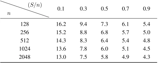
Table 1:Maximum value of the ratioσe/σato recover aSsparse secret in dimensionnwith the Dantzig selector
n
(S/n)
0.1 0.3 0.5 0.7 0.9
128 16.2 9.4 7.3 6.1 5.4
256 15.2 8.8 6.8 5.7 5.0
512 14.3 8.3 6.4 5.4 4.8
1024 13.6 7.8 6.0 5.1 4.5
2048 13.0 7.5 5.8 4.9 4.3
Let us discuss the practicality of this approach with regards to the parameters of the ILWE problem. First of all, note that in order to make Condition (4.13) non-vacuous, one needsσeandσato satisfy:
2C1
r
2 logn
n ≤
σa σe
≤2C1
p
2 logn,
where the lower bound follows from the fact thatSis a positive integer, and the upper bound from the observation that the right-hand side of (4.13) must be smaller thannto be of any interest compared to the trivial boundS ≤n. Practically speaking, this means that this approach is only interesting when the ratioσe/σais relatively small; concrete bounds are provided in Table1various sparsity levels and dimensions ranging from128to2048.
We note that the required sparsity is much higher than proposed parameters for BLISS, for example. Moreover, the complexity of this linear programming based approach is worse than least squares regression. However, only this method is applicable when onlym < nsamples are available.
5
Application to the Side-channel Attack of BLISS
5.1 BLISS Signatures and Rejection Sampling Leakage
The BLISS signature scheme [31] is a lattice-based signature scheme based on the Ring-Learning With Error (RLWE) assumption. Its signing algorithm is recalled in Figure1.
The rejection sampling. The BLISS signature scheme follows the “Fiat–Shamir with aborts” paradigm of Lyuba-shevsky [34]. In particular, signature generation involves arejection samplingstep (Step8of function SIGNin Fig-ure1) which is essential for security: in order to ensure that the distribution of signatures is independent of the secret keys= (s1,s2), a signature candidate z= (z1,z2),c
should be kept with probability
1
,
Mexp
−ksck 2
2σ2
cosh
hz,sci
σ2
!
.
16
Fig. 1:BLISS signing algorithm. The hash functionHis modeled as a RO with values in the set of polynomials inRwith 0/1-coefficient and Hamming weightκ. See [31] for details regarding notation likeζ,d·cdandpnot discussed in this paper.
1: functionSIGN(µ, pk=v1,sk=s= (s1,s2)) 2: y1,y2←Dσn¯
3: u=ζ·v1·y1+y2 mod 2q
4: c←H(ducd modp, µ) 5: choose a random bitb
6: z1←y1+ (−1)bs1c 7: z2←y2+ (−1)bs2c
8: continuewith probability1/ Mexp(−ksck2
/(2σ2)) cosh(hz,sci/σ2
; otherwiserestart
9: z†2←(ducd− du−z2cd) modp 10: return(z1,z†2,c)
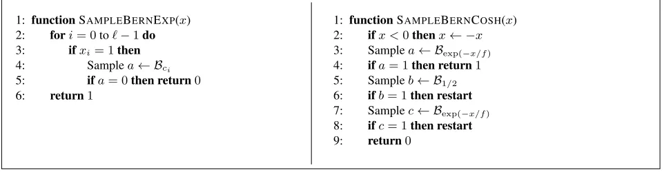
Fig. 2:Sampling algorithms for the distributionsBexp(−x/2σ2) andB1/cosh(x/σ2). The valuesci = 2i/f precomputed, and the
xi’s are the bits in the binary expansion ofx=P`−1 i=02
i
xi. BLISS usesx=K− ksck2
for the input to the exponential sampler, andx= 2hz,scifor the input to thecoshsampler.
1: functionSAMPLEBERNEXP(x) 2: fori= 0to`−1do
3: ifxi= 1then 4: Samplea← Bci 5: ifa= 0then return0 6: return1
1: functionSAMPLEBERNCOSH(x) 2: ifx <0thenx← −x
3: Samplea← Bexp(−x/f) 4: ifa= 1then return1 5: Sampleb← B1/2 6: ifb= 1then restart
7: Samplec← Bexp(−x/f) 8: ifc= 1then restart
9: return0
Side-channel leakage of the rejection sampling. Based on their description in Figure2, it is clear that SAMPLEBERNEXP and SAMPLEBERNCOSHdo not run in constant time. In fact, they iterate over the bits of their input, and part of the code is executed when the bit is1and skipped over when the bit is0. As a result, as observed by Espitau et al. [30,§3], the inputsxexp, xcoshof these functions can be read off directly on a trace of power consumption or electromagnetic emanations, in much the same way as naive square-and-multiply implementations of RSA leak the secret exponent via simple power analysis [46,§3.1]. As a result, side-channel analysis allows to reliably recover the squared norm ksck2=ks1ck2+ks2ck2and the scalar producthz,sci=hz1,s1ci+hz2,s2cifrom generated signatures.
Espitau et al. show that the norm leakage can be leveraged in practice to recover the secret key from a little over¯nsignature traces, wheren¯ is the extension degree of the ringR(n¯ = 512for the most common parameters). However, the recovery technique is mathematically quite involved and computationally costly (it is based on the Howgrave-Graham–Szydlo solution to cyclotomic norm equations [47], and takes over a month of CPU time for typical parameters). More importantly, it has the major drawback of relying on the ability to factor this norm and thus only applying to “weak” signing keys satisfying a certain semismoothness condition (around7%of BLISS secret keys).
17 5.2 Description of the Attack
As we have mentioned already, recovering the secrets∈Z2¯n =
Znfrom the linear leakagehz,sciessentially amounts to an instance of the ILWE problem. We now describe more precisely in what sense. To do so, we need to write this inner product in terms of the known ring elements(c,z1,z†2)that appear in the signature on the one hand, and unknown elements on the other hand. This can be done as follows:
hz,sci=hz1,s1ci+hz2,s2ci=hz1c∗,s1i+h2dz†2,s2ci+hz2−2dz†2,s2ci
=hz1c∗,s1i+h2dz2†c∗,s2i+e=ha,si+e, where we let:
a= (z1c∗,2dz†2c∗)∈Z2¯n=Zn and e=hz2−2dz†2,s2ci.
The vectoracan be computed from the signature, and is therefore known to the side-channel attacker, whereaseis some unknown value. In these expressions,c∗is the conjugate ofcwith respect to the inner product (i.e. the matrix of multiplication bycin the polynomial basis ofZ[x]/(xn¯+ 1)is the transpose of that ofc).
Now the rejection sampling ensures that the coefficients of z1 are independent and distributed according to a discrete GaussianDof standard deviationσ. On the other hand,cis a random vector with coefficients in{0,1}and exactlyκnon zero coefficients; thus,c∗has a similar shape possibly up to the sign of coefficients. It follows that the coefficients ofz1c∗are all linear combinations with±1coefficients of exactlyκindependent samples fromDand the signs clearly do not affect the resulting distribution.
Therefore, if we denote by χa the distributionD∗κ obtained by summingκindependent samples fromD, the coefficients ofz1c∗ followχa. It is not exactly correct thatz1c∗ as a whole followsχ¯na (as its coefficients are not rigorously independent), but we will heuristically ignore that subtlety and pretend it does. Note thatχais a distribution of variance:
σ2a= Var D∗ κ
=κ·Var(D) =κσ2.
We have not precisely described how the BLISS signature compression works, but roughly speaking,z†2is essentially obtained by keeping the(logq−d)most significant bits ofz2, and therefore the distribution of2dz†2is close to that of z2. The distributions cannot coincide exactly, since all the coefficients of2dz†2are multiples of2dwhile this normally does not happen forz2, but the difference will not matter much for our purposes, and we will therefore heuristically assume that the entire vectorais distributed asχn
a.
We now turn our attention to the noise valuee, which we write ashw,uiwithw=z2−2dz†2andu=s2c. Now, wis obtained as the difference betweenz2and2dz†2, where again the latter is roughly speaking obtained by zeroing out thedleast significant bits ofz2in a centered way. We can therefore heuristically expect that the coefficients ofw are distributed uniformly in[−2d−1,2d−1]∩Z, i.e.w ∼ Uαn withα= 2d−1. In particular, these coefficients have varianceα(α+ 1)/3≈22d/12.
As for u, its coefficients are obtained as sums ofκcoefficients ofs2. Nows2 itself (ignoring the constant co-efficient, which is shifted by1) is obtained as a random vector with δ1n¯ coefficients equal to±2,δ2n¯ coefficients equal to±4and all its other coefficients equal to zero. This is a somewhat complicated distribution to describe, but we do not make a large approximation by pretending that all the coefficients are sampled independently in the set {−4,−2,0,2,4}with probabilitiesδ2/2, δ1/2,(1−δ1−δ2), δ1/2andδ2/2respectively. Making that approximation, it follows that the coefficients ofuhave varianceκ·(4δ1+ 16δ2).
Writeu = (u1, . . . , un¯)andw = (w1, . . . , wn¯). Under the heuristic approximations above, sincewanduare independent and their coefficients have mean zero, the errorefollows a certain bounded distributionχeof varianceσ2e given by:
σ2e=E[e2] =E
Xn¯
i=1 wiui
2
=E
X
i,j
wiwjuiuj
=E
n¯ X
i=1 w2iu2i
=
¯ n
X
i=1
E[w2i]·E[u2i] = ¯n·Var Uα
·κ(4δ1+ 16δ2)≈
22d
18
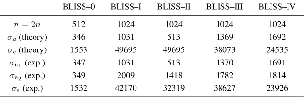
Table 2:Parameter estimation for ILWE instances arising from the side channel attack
BLISS–0 BLISS–I BLISS–II BLISS–III BLISS–IV
n= 2¯n 512 1024 1024 1024 1024
σa(theory) 346 1031 513 1369 1692
σe(theory) 1553 49695 49695 38073 24535
σa1(exp.) 347 1031 513 1370 1691
σa2(exp.) 349 2009 1418 1782 1814
σe(exp.) 1532 42170 32319 38627 23926
With these various approximations, recoveringsfrom the leakage exactly becomes an ILWE problem with distri-butionsχaandχe, where each side-channel trace provides a sample. It should therefore be feasible to recover the full secret key with least squares regression usingm=O (σe/σa)2logntraces.
5.3 Experimental Distributions
The description of the previous section made a number of heuristic approximations which we know cannot be precisely satisfied in practice. In order to validate those approximations nonetheless, we have carried out numerical simulations comparing in particular our estimates for the standard deviationsσa andσeof the distributions ofaandewith the standard deviations obtained from the actual rejection sampling leakage in BLISS.
These simulations were carried out in Python using the numpy package. We used 10000 ILWE samples arising from side channel leaks for each BLISS parameter set. Results are collected in Table2; experimental values forσaare provided separately for the two halves(a1,a2)of the vectora, which we have seen are computed differently. As we can see, the experimental values match the heuristic estimates quite closely overall.
6
Numerical Simulations
In this section, we present simulation results for recovering ILWE secrets using linear regression, first for normal ILWE instances, and then for ILWE instances arising from BLISS side-channel leakage, as described in§5.2, leading to BLISS secret key recovery. These results are based on simulated leakage data rather than actual side-channel traces. However, we note that the leakage scenario for BLISS is essentially identical to the one described in [30] (namely, a SPA/SEMA setting where each trace reveals the exact value of a certain function of the secret key—in our case, the linear function given by the inner product), and was therefore experimentally validated in that paper.
6.1 Plain ILWE
Recall that the ILWE problem is parametrized by n, m ∈ Zand probability distributions χa andχe. Samples are computed asb=As+e, wheres∈Zn,b∈Zm,A∈Zm×nwith entries drawn fromχa, ande∈Zmwith entries drawn fromχe. Choosingχaandχeas discrete gaussian distributions with standard deviationsσaandσerespectively, we investigated the number of samples,mrequired to recover ILWE secret vectorss∈Znfor various concrete values ofn, σaandσe. We sampled sparse secret vectorssuniformly at random from the set of vectors withd0.15neentries set to±1,d0.15neentries set to±2, and the rest zero.
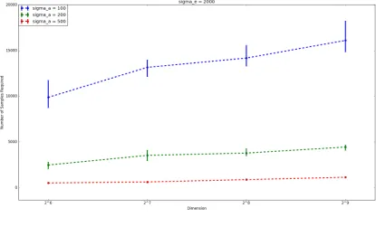
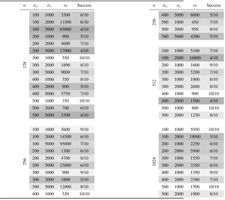
We present two types of experimental results for plain ILWE. In our first experiment, we began by estimating the number of samplesmrequired to recover the secret perfectly with good probability, for different values ofn, σa, and σe. Then, fixingm, we measured the probability of recoveringsover the random choices ofs,Aande. Our results are displayed in Table3.
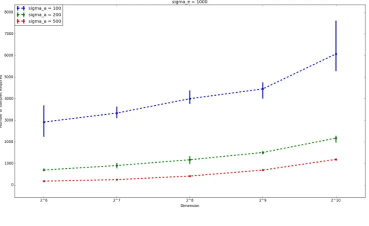
19 other words, for fixedn, σa, andσe, we generated more and more samples until the secret could be perfectly recovered. Our results forσe = 2000are plotted in Figure3. Additional results comprising Figures4,5and6, forσe= 1000,
3000and5000respectively,and some additional notes,may be found in AppendixB. Each figure plots the dimension nagainst the mean number of samplesmrequired to recover the secret, forσa = 100,200, and500. Here, ‘mean’ refers to the interquartile mean number of samples. The error bars show the upper and lower quartiles for the number of samples required.
The results of our second experiment are consistent with the theoretical results given in§4.1. According to (4.6), we require
m≥C0·σ 2 e σ2 a
logn
samples in order to recover the secret correctly. The dimensionnon the horizontal axis of each graph is plotted on a logarithmic scale. Therefore, theory predicts that we should observe a straight line, which the graphs confirm.
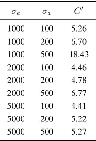
The gradient of the graph corresponds to the constantC0giving the number of samples required for secret-recovery in practice. Note that in this case, where χa andχe follow the discrete Gaussian distribution, Theorem 4.5gives C0 = 32for a small failure probability of 2n1. However, in this experiment, we are likely to succeed much sooner, with a smaller number of samples. For example, in any particular trial, as soon asmis such that the failure probability is at least one half, we are likely to recover the secret. This explains why the gradient is much lower than given by Theorem4.5. Computing the gradients of the lines of best fit and dividing by(σe/σa)2 gives an estimate for the observed value of the constantC0. These are displayed in Table6in AppendixB, and indicate that one might expect to use4≤C0 ≤6in practice.
20
Table 3:Practical results of the experiments on ILWE
n σa σe m Success
100 1000 3300 6/10
100 2000 11500 6/10
100 5000 65000 4/10
200 1000 900 5/10
200 2000 4000 7/10
200 5000 17000 4/10
300 1000 550 10/10
300 2000 1890 8/10
300 5000 9000 7/10
400 1000 350 8/10
400 2000 800 5/10
400 5000 5750 7/10
500 1000 350 10/10
500 2000 700 6/10
128
500 5000 3300 4/10
100 1000 5600 9/10
100 2000 14500 6/10
100 5000 95000 7/10
200 1000 1300 6/10
200 2000 4700 8/10
200 5000 23000 6/10
300 1000 900 9/10
300 2000 1800 5/10
300 5000 12000 8/10
256
400 1000 550 10/10
n σa σe m Success
400 5000 6000 5/10
500 1000 450 7/10
500 2000 950 8/10
256
500 5000 4200 5/10
100 1000 5100 7/10
100 2000 16000 4/10
200 1000 1600 9/10
200 2000 5200 7/10
300 1000 1000 8/10
300 2000 2600 8/10
400 1000 900 10/10
400 2000 1500 4/10
500 1000 800 10/10
512
500 2000 1250 8/10
100 1000 5950 10/10
100 2000 19000 5/10
200 1000 2250 6/10
200 2000 5900 6/10
300 1000 1550 7/10
300 2000 3350 6/10
400 1000 1350 9/10
400 2000 2300 7/10
500 1000 1500 10/10
1024
21
Table 4:Number of samples required to recover the secret key (minimum, lower quartile, interquartile mean, upper quartile, maxium)
# Trials Min LQ IQM UQ Max
BLISS–0 12 1203 1254 1359.5 1515 1641 BLISS–I 12 14795 18648 20382.9 21789 24210 BLISS–II 8 19173 20447 22250.3 24482 29800
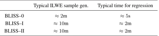
Table 5:Typical timings for secret key recovery
Typical ILWE sample gen. Typical time for regression
BLISS–0 ≈2m ≈5s
BLISS–I ≈10m ≈2m
BLISS–II ≈10m ≈2m
6.2 BLISS Side-Channel Attack
Having obtained an instance of the ILWE problem from BLISS side-channel leakage as described in§5.2, we used linear regression to recover BLISS secret keys. We performed several trials. For each trial, we generated ILWE samples using side-channel leakage until we could recover the secret key. For BLISS–0, we simply used regression to recover the entire secret key. For BLISS–I and BLISS–II, we usually ran into memory issues before being able to successfully recover the entire secret key. However, we noticed that in practice, we could recover the first half of the secret key correctly using far fewer samples. Since the two halves of the secret key are related by the public key, this is sufficient to compute the entire secret key. Therefore, for BLISS–I and BLISS–II, we stopped generating samples as soon as the least-squares estimator correctly recovered the first half of the secret.
For these two different scenarios, we obtain the results displayed on Table4, which gives information on the range, quartiles, and interquartile mean of the number of samples required. Typical timings for the side-channel attacks, using SAGEMath, on a laptop with 2.60GHz processor, are displayed in Table5. Timings are in the orders of minutes and seconds. By comparison, some of the attacks from [30] may take hours, or even days, of CPU time.
References
1. Regev, O.: On lattices, learning with errors, random linear codes, and cryptography. In Gabow, H.N., Fagin, R., eds.: 37th ACM STOC, ACM Press (May 2005) 84–93
2. Arora, S., Ge, R.: New algorithms for learning in presence of errors. In Aceto, L., Henzinger, M., Sgall, J., eds.: ICALP 2011, Part I. Volume 6755 of LNCS., Springer, Heidelberg (July 2011) 403–415
3. Micciancio, D., Peikert, C.: Hardness of SIS and LWE with small parameters. In Canetti, R., Garay, J.A., eds.: CRYPTO 2013, Part I. Volume 8042 of LNCS., Springer, Heidelberg (August 2013) 21–39
4. D¨ottling, N., M¨uller-Quade, J.: Lossy codes and a new variant of the learning-with-errors problem. In Johansson, T., Nguyen, P.Q., eds.: EUROCRYPT 2013. Volume 7881 of LNCS., Springer, Heidelberg (May 2013) 18–34
5. Applebaum, B., Cash, D., Peikert, C., Sahai, A.: Fast cryptographic primitives and circular-secure encryption based on hard learning problems. In Halevi, S., ed.: CRYPTO 2009. Volume 5677 of LNCS., Springer, Heidelberg (August 2009) 595–618 6. Brakerski, Z., Langlois, A., Peikert, C., Regev, O., Stehl´e, D.: Classical hardness of learning with errors. In Boneh, D.,
Roughgarden, T., Feigenbaum, J., eds.: 45th ACM STOC, ACM Press (June 2013) 575–584
7. Albrecht, M.R., Faug`ere, J.C., Fitzpatrick, R., Perret, L.: Lazy modulus switching for the BKW algorithm on LWE. In Krawczyk, H., ed.: PKC 2014. Volume 8383 of LNCS., Springer, Heidelberg (March 2014) 429–445
229. Albrecht, M.R.: On dual lattice attacks against small-secret LWE and parameter choices in HElib and SEAL. In Coron, J.,
Nielsen, J.B., eds.: EUROCRYPT 2017, Part II. Volume 10211 of LNCS., Springer, Heidelberg (April / May 2017) 103–129 10. Galbraith, S.D.: Space-efficient variants of cryptosystems based on learning with errors. On-Line (2012)https://www.
math.auckland.ac.nz/˜sgal018/compact-LWE.pdf.
11. Herold, G., May, A.: LP solutions of vectorial integer subset sums — cryptanalysis of Galbraith’s binary matrix LWE. In Fehr, S., ed.: PKC 2017, Part I. Volume 10174 of LNCS., Springer, Heidelberg (March 2017) 3–15
12. Goldwasser, S., Kalai, Y.T., Peikert, C., Vaikuntanathan, V.: Robustness of the learning with errors assumption. In Yao, A.C.C., ed.: ICS 2010, Tsinghua University Press (January 2010) 230–240
13. Dodis, Y., Goldwasser, S., Kalai, Y.T., Peikert, C., Vaikuntanathan, V.: Public-key encryption schemes with auxiliary inputs. In Micciancio, D., ed.: TCC 2010. Volume 5978 of LNCS., Springer, Heidelberg (February 2010) 361–381
14. Ling, S., Phan, D.H., Stehl´e, D., Steinfeld, R.: Hardness of k-LWE and applications in traitor tracing. In Garay, J.A., Gennaro, R., eds.: CRYPTO 2014, Part I. Volume 8616 of LNCS., Springer, Heidelberg (August 2014) 315–334
15. Lyubashevsky, V., Peikert, C., Regev, O.: On ideal lattices and learning with errors over rings. In Gilbert, H., ed.: EURO-CRYPT 2010. Volume 6110 of LNCS., Springer, Heidelberg (May / June 2010) 1–23
16. Stehl´e, D., Steinfeld, R., Tanaka, K., Xagawa, K.: Efficient public key encryption based on ideal lattices. In Matsui, M., ed.: ASIACRYPT 2009. Volume 5912 of LNCS., Springer, Heidelberg (December 2009) 617–635
17. Lyubashevsky, V., Peikert, C., Regev, O.: A toolkit for ring-LWE cryptography. In Johansson, T., Nguyen, P.Q., eds.: EURO-CRYPT 2013. Volume 7881 of LNCS., Springer, Heidelberg (May 2013) 35–54
18. Langlois, A., Stehl´e, D.: Worst-case to average-case reductions for module lattices. Designs, Codes and Cryptography75(3) (2015) 565–599
19. Banerjee, A., Peikert, C., Rosen, A.: Pseudorandom functions and lattices. In Pointcheval, D., Johansson, T., eds.: EURO-CRYPT 2012. Volume 7237 of LNCS., Springer, Heidelberg (April 2012) 719–737
20. Alwen, J., Krenn, S., Pietrzak, K., Wichs, D.: Learning with rounding, revisited - new reduction, properties and applications. In Canetti, R., Garay, J.A., eds.: CRYPTO 2013, Part I. Volume 8042 of LNCS., Springer, Heidelberg (August 2013) 57–74 21. Bogdanov, A., Guo, S., Masny, D., Richelson, S., Rosen, A.: On the hardness of learning with rounding over small modulus. In
Kushilevitz, E., Malkin, T., eds.: TCC 2016-A, Part I. Volume 9562 of LNCS., Springer, Heidelberg (January 2016) 209–224 22. Liu, D.: Compact-LWE for lightweight public key encryption and leveled IoT authentication. In Pierpzyk, J., Suriadi, S., eds.:
ACISP 17, Part I. Volume 10342 of LNCS., Springer, Heidelberg (July 2017) xvi
23. Liu, D., Li, N., Kim, J., Nepal, S.: Compact-LWE (2017) https://csrc.nist.gov/projects/ post-quantum-cryptography/round-1-submissions.
24. Bootle, J., Tibouchi, M., Xagawa, K.: Cryptanalysis of Compact-LWE. In Smart, N.P., ed.: CT-RSA. Volume 10808 of LNCS., Springer (2018) 80–97
25. Xiao, D., Yu, Y.: Cryptanalysis of Compact-LWE and related lightweight public key encryption. Security and Communication Networks2018(2018)
26. Li, H., Liu, R., Pan, Y., Xie, T.: Cryptanalysis of Compact-LWE submitted to NIST PQC project. Cryptology ePrint Archive, Report 2018/020 (2018)https://eprint.iacr.org/2018/020.
27. Hoffstein, J., Pipher, J., Whyte, W., Zhang, Z.: A signature scheme from learning with truncation. Cryptology ePrint Archive, Report 2017/995 (2017)http://eprint.iacr.org/2017/995.
28. Hamburg, M.: Post-quantum cryptography proposal: ThreeBears (2017) https://csrc.nist.gov/projects/ post-quantum-cryptography/round-1-submissions.
29. Aggarwal, D., Joux, A., Prakash, A., Santha, M.: A new public-key cryptosystem via Mersenne numbers. Cryptology ePrint Archive, Report 2017/481 (2017)http://eprint.iacr.org/2017/481.
30. Espitau, T., Fouque, P.A., G´erard, B., Tibouchi, M.: Side-channel attacks on BLISS lattice-based signatures: Exploiting branch tracing against strongSwan and electromagnetic emanations in microcontrollers. In Thuraisingham, B.M., Evans, D., Malkin, T., Xu, D., eds.: ACM CCS 17, ACM Press (October / November 2017) 1857–1874
31. Ducas, L., Durmus, A., Lepoint, T., Lyubashevsky, V.: Lattice signatures and bimodal Gaussians. In Canetti, R., Garay, J.A., eds.: CRYPTO 2013, Part I. Volume 8042 of LNCS., Springer, Heidelberg (August 2013) 40–56
32. Bruinderink, L.G., H¨ulsing, A., Lange, T., Yarom, Y.: Flush, gauss, and reload - A cache attack on the BLISS lattice-based signature scheme. In Gierlichs, B., Poschmann, A.Y., eds.: CHES 2016. Volume 9813 of LNCS., Springer, Heidelberg (August 2016) 323–345
33. Pessl, P., Bruinderink, L.G., Yarom, Y.: To BLISS-B or not to be: Attacking strongSwan’s implementation of post-quantum signatures. In Thuraisingham, B.M., Evans, D., Malkin, T., Xu, D., eds.: ACM CCS 17, ACM Press (October / November 2017) 1843–1855
34. Lyubashevsky, V.: Fiat-Shamir with aborts: Applications to lattice and factoring-based signatures. In Matsui, M., ed.: ASI-ACRYPT 2009. Volume 5912 of LNCS., Springer, Heidelberg (December 2009) 598–616
23 36. Kahane, J.P.: Propri´et´es locales des fonctions `a s´eries de Fourier al´eatoires. Stu. Math.19(1960) 1–25
37. Tropp, J.A.: User-friendly tail bounds for sums of random matrices. Foundations of Computational Mathematics12(4) (Aug 2012) 389–434
38. Hsu, D., Kakade, S., Zhang, T.: Tail inequalities for sums of random matrices that depend on the intrinsic dimension. Electron. Commun. Probab.17(2012) 13 pp.
39. Litvak, A., Pajor, A., Rudelson, M., Tomczak-Jaegermann, N.: Smallest singular value of random matrices and geometry of random polytopes. Advances in Mathematics195(2) (2005) 491–523
40. Stadje, W.: An inequality for`p-norms with respect to the multivariate normal distribution. Journal of Mathematical Analysis and Applications102(1) (1984) 149 – 155
41. Ramon van Handel: Probability in high dimension. Technical report, Princeton University (2014)
42. Paouris, G., Valettas, P., Zinn, J.: Random version of Dvoretzky’s theorem in`np. Stochastic Processes and their Applications
127(10) (2017) 3187–3227
43. Ducas, L., Lepoint, T.: BLISS: Bimodal lattice signature schemes (June 2013) (proof-of-concept implementation).
44. P¨oppelmann, T., Oder, T., G¨uneysu, T.: High-performance ideal lattice-based cryptography on 8-bit ATxmega microcontrollers. In Lauter, K.E., Rodr´ıguez-Henr´ıquez, F., eds.: LATINCRYPT 2015. Volume 9230 of LNCS., Springer, Heidelberg (August 2015) 346–365
45. Steffen, A., et al.: strongSwan: the open source IPsec-based VPN solution (version 5.5.2) (March 2017)
46. Kocher, P.C., Jaffe, J., Jun, B., Rohatgi, P.: Introduction to differential power analysis. J. Cryptographic Engineering1(1) (2011) 5–27
47. Howgrave-Graham, N., Szydlo, M.: A method to solve cyclotomic norm equations. In Buell, D.A., ed.: ANTS. Volume 3076 of LNCS., Springer (2004) 272–279
48. Peikert, C.: An efficient and parallel Gaussian sampler for lattices. In Rabin, T., ed.: CRYPTO 2010. Volume 6223 of LNCS., Springer, Heidelberg (August 2010) 80–97
49. Micciancio, D., Regev, O.: Worst-case to average-case reductions based on Gaussian measures. In: 45th FOCS, IEEE Computer Society Press (October 2004) 372–381