Polynomially Adjusted Saddlepoint Density Approximations

(1)

Western University Western University

Scholarship@Western

Electronic Thesis and Dissertation Repository

11-18-2013 12:00 AM

Polynomially Adjusted Saddlepoint Density Approximations

Susan Zhe Sheng

The University of Western Ontario

Supervisor Dr. Serge Provost

The University of Western Ontario

Graduate Program in Statistics and Actuarial Sciences

A thesis submitted in partial fulfillment of the requirements for the degree in Doctor of Philosophy

Follow this and additional works at: https://ir.lib.uwo.ca/etd

Part of the Applied Statistics Commons, and the Statistical Methodology Commons

Recommended Citation Recommended Citation

Sheng, Susan Zhe, "Polynomially Adjusted Saddlepoint Density Approximations" (2013). Electronic Thesis and Dissertation Repository. 1709.

https://ir.lib.uwo.ca/etd/1709

This Dissertation/Thesis is brought to you for free and open access by Scholarship@Western. It has been accepted for inclusion in Electronic Thesis and Dissertation Repository by an authorized administrator of

(2)

POLYNOMIALLY ADJUSTED SADDLEPOINT DENSITY

APPROXIMATIONS

(Thesis format: Monograph)

by

Susan Zhe Sheng

Graduate Program in Statistics and Actuarial Science

A thesis submitted in partial fulfillment

of the requirements for the degree of

Doctor of Philosophy

The School of Graduate and Postdoctoral Studies

The University of Western Ontario

London, Ontario, Canada

c

(3)

Abstract

This thesis aims at obtaining improved bona fide density estimates and approximants by means of adjustments applied to the widely used saddlepoint approximation. Said adjustments are determined by solving systems of equations resulting from a moment-matching argument. A hybrid density approximant that relies on the accuracy of the saddlepoint approximation in the distributional tails is introduced as well. A certain representation of noncentral indefinite quadratic forms leads to an initial approximation whose parameters are evaluated by simul-taneously solving four equations involving the cumulants of the target distribution. A sad-dlepoint approximation to the distribution of quadratic forms is also discussed. By way of application, accurate approximations to the distributions of the Durbin-Watson statistic and a certain portmanteau test statistic are determined. It is explained that the moments of the latter can be evaluated either by defining an expected value operator via the symbolic approach or by resorting to a recursive relationship between the joint moments and cumulants of sums of products of quadratic forms. As well, the bivariate case is addressed by applying a polynomial adjustment to the product of the saddlepoint approximations of the marginal densities of the standardized variables. Furthermore, extensions to the context of density estimation are formu-lated and applied to several univariate and bivariate data sets. In this instance, sample moments and empirical cumulant-generating functions are utilized in lieu of their theoretical analogues. Interestingly, the methodology herein advocated for approximating bivariate distributions not only yields density estimates whose functional forms readily lend themselves to algebraic ma-nipulations, but also gives rise to copula density functions that prove significantly more flexible than the conventional functional type.

(4)

(5)

ACKNOWLEDGEMENTS

There are many people I would like to thank for their support over the past three years.

Firstly, I would like to express my gratitude to my supervisor, Dr. Serge Provost, for his valuable guidance, as well as his patience and keen enthusiasm to make this thesis possible.

I would also like to thank my thesis examiners, Professors Jiandong Ren, B. M. Golam Kibria, John Koval and Ri˜cardas Zitikis for their suggestions. Many thanks to my office mates, Yanyan, Candy and Huan, for providing a nice atmosphere over the last two years. I am grateful to all people in the Department of Statistical and Actuarial Sciences for their kindness and friendship. A special thanks to Monty for his support.

(6)

List of Figures

2.1 Saddlepoint approximation (dark line) and polynomially adjusted saddlepoint approximation of degree 8 (dashed line) superimposed on the triangular density (grey line) . . . 8

2.2 Saddlepoint approximation (dark line) and polynomially adjusted saddlepoint approximation of degree 16 (dashed line) superimposed on the triangular den-sity (grey line) . . . 9

2.3 Saddlepoint approximation (dark line) and polynomially adjusted saddlepoint approximation of degree 2 (dashed line) superimposed on the sinusoidal den-sity (grey line) . . . 11

2.4 Saddlepoint approximation (dark line) and polynomially adjusted saddlepoint approximation of degree 8 (dashed line) superimposed on the Weibull density (grey line) . . . 13

2.5 Saddlepoint approximation (dark line) and polynomially adjusted saddlepoint approximation of degree 16 (dashed line) superimposed on the mixture of beta densities (grey line) . . . 15

2.6 Saddlepoint approximation (dark line) and polynomially adjusted saddlepoint approximation of degree 16 (dashed line) superimposed on the mixture of beta densities (grey line) . . . 15

2.7 Saddlepoint approximation (dark line) and polynomially adjusted saddlepoint approximation of degree 12 (dashed line) superimposed on the mixture of nor-mal densities (grey line) . . . 17

2.8 Saddlepoint approximation (dark line) and polynomially adjusted saddlepoint approximation of degree 16 (dashed line) superimposed on the mixture of gamma densities (grey line) . . . 21

2.9 Saddlepoint approximation adjusted by a ratio of polynomials of degrees 3 and 2 (dashed line) superimposed on the Weibull density (grey line) . . . 22

(10)

3.1 Gamma Density Approximant forQ4 . . . 39

3.2 Gamma cdf approximation (dots) and simulated cdf forQ4 . . . 40

3.3 First transformed gamma CDF approximation (black line), second transformed gamma CDF approximation (dots) and proposed polynomially adjusted beta CDF approximation (large dots) superimposed on the simulated CDF (in grey) forn=10 andm= 3 [Normal process] . . . 54 3.4 First transformed gamma CDF approximation (black line) and proposed

poly-nomially adjusted beta CDF approximation (large dots) superimposed on the simulated CDF (in grey) forn=10 andm= 3 [MA(1) process] . . . 54 3.5 First transformed gamma CDF approximation (black line) and proposed

poly-nomially adjusted beta CDF approximation (large dots) superimposed on the simulated CDF (in grey) forn=10 andm= 3 [AR(1) process] . . . 54 3.6 First transformed gamma CDF approximation (black line), second transformed

gamma CDF approximation (dots) and Proposed Polynomially Adjusted Beta CDF approximation (large dots) superimposed on the simulated CDF (in grey) forn=36 andm= 12 [Normal process] . . . 55 3.7 First transformed gamma CDF approximation (black line), second transformed

gamma CDF approximation (dots) and beta CDF approximation (large dots) superimposed on the simulated CDF (in grey) forn = 36 andm= 12 [MA(1) process] . . . 55

3.8 First transformed gamma CDF approximation (black line), second transformed gamma CDF approximation (dots) and beta CDF approximation (large dots) superimposed on the simulated CDF (in grey) forn = 36 and m = 12 [AR(1) process] . . . 55

3.9 First transformed gamma CDF approximation (black line), second transformed gamma CDF approximation (dots) and beta CDF approximation (large dots) superimposed on the simulated CDF (in grey) forn= 36 andm= 12 [ARMA(1,1) process] . . . 55

3.10 First transformed gamma CDF approximation (black line) and beta CDF ap-proximation (large dots) superimposed on the simulated CDF (in grey) for n=36 andm=12 [ARMA(2,2) process] . . . 56 3.11 Adjusted saddlepoint approximation (large dots) superimposed on the

simu-lated CDF (in grey) forn= 10 andm= 3 [normal process] . . . 56 3.12 Adjusted saddlepoint approximation (large dots) superimposed on the

(11)

3.13 Adjusted saddlepoint approximation (large dots) superimposed on the

simu-lated CDF (in grey) forn= 10 andm= 3 [AR(1) process] . . . 56

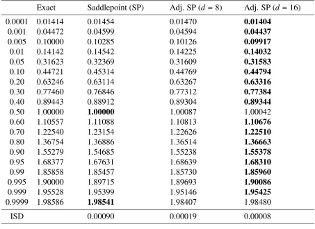
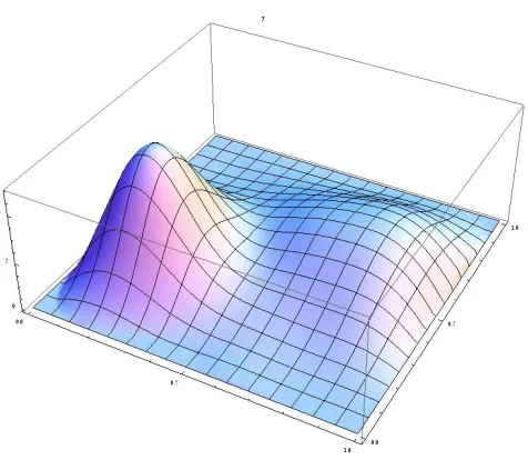
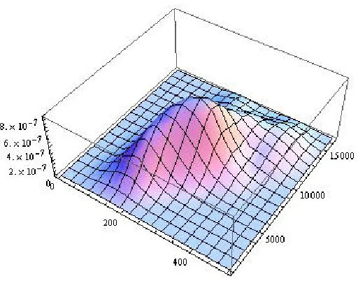
4.1 The pdf of the mixture of three normal densities . . . 62

4.2 The pdf of the standardized mixture of three normal densities . . . 63

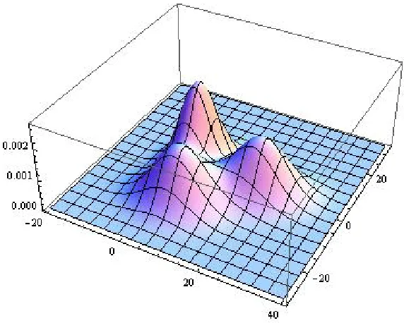
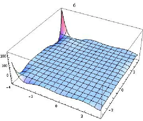
4.3 The product of the marginal pdf’s of the standardized mixture of three normal densities . . . 64

4.4 The polynomial adjustment (t=6) of the standardized mixture of three normal densities . . . 64

4.5 The polynomially adjusted pdf approximation (t=6) of the standardized mix-ture of three normal densities . . . 65

4.6 The polynomially adjusted pdf approximation (t= 6) of the mixture of three normal densities after applying the inverse transformation . . . 65

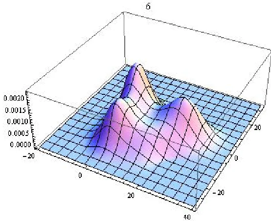
4.7 The pdf of the mixture of two beta densities . . . 66

4.8 The product of the marginal pdfs of the mixture of two beta densities . . . 66

4.9 The polynomially adjustment (t=7) of the mixture of two beta densities . . . . 67

4.10 The polynomially adjusted pdf (t=7) of the mixture of two beta densities . . . 67

5.1 Histogram of the Buffalo snowfall data with saddlepoint estimate (dashed line) and kernel density estimate (black line) . . . 69

5.2 The empirical saddlepoint CDF estimate, with an 10th degree polynomial ad-justment (dashed line) and kernel density estimate (black line) superimposed on the empirical CDF of the Buffalo snowfall data . . . 70

5.3 Histogram of the flood data with saddlepoint estimate (dashed line) and kernel density estimate (black line) . . . 71

5.4 The empirical saddlepoint CDF estimate, with an 8th _{degree polynomial} ad-justment (dashed line) and kernel density estimate (black line) superimposed on the empirical CDF of the flood data . . . 71

5.5 Histogram of the Chicago data with saddlepoint estimate (dashed line) and kernel density estimate (black line) . . . 72

5.6 The empirical saddlepoint CDF estimate, with an 8th degree polynomial ad-justment (dashed line) and kernel density estimate (black line) superimposed on the empirical CDF of the Chicago data . . . 72

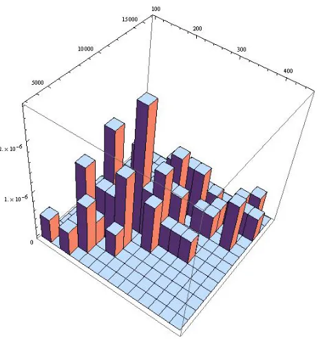
5.7 Histogram of the bivariate flood data . . . 73

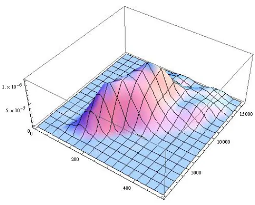
5.8 Product of the marginal densities of the standardized flood data . . . 74

(12)

5.11 Adjusted saddlepoint density estimate of the original flood data after applying

the inverse transformation . . . 75

5.12 Kernel density estimate for the flood data . . . 76

5.13 Histogram of the Old Faithful data . . . 77

5.14 Product of the marginal densities for the standardized Old Faithful data . . . 77

5.15 Polynomial adjustment of the standardized Old Faithful data (t=6) . . . 78

5.16 The adjusted bivariate saddlepoint density estimate of the standardized Old Faithful data (t= 6) . . . 78

5.17 Saddlepoint density estimate of the original Old Faithful data, after applying the inverse transformation . . . 79

5.18 Kernel density estimate of the Old Faithful data . . . 79

5.19 Histogram of the Chicago data . . . 80

5.20 Product of the marginal densities for the standardized Chicago data . . . 81

5.21 Polynomial adjustment of the standardized Chicago data (t=6) . . . 81

5.22 The adjusted bivariate saddlepoint density estimate approximation of the stan-dardized Chicago data (t=6) . . . 82

5.23 The adjusted saddlepoint density estimate of the original Chicago data, after applying the inverse transformation . . . 82

5.24 Kernel density estimate of the Chicago data . . . 83

6.1 Histogram of the standardized flood data . . . 90

6.2 The adjusted bivariate density estimate for the standardized flood data (t=5) . 90 6.3 The empirical cumulative distribution function of the standardized flood data . . 91

6.4 The copula as determined from Deheuvels’ formula . . . 91

6.5 The copula density estimate of the flood data as obtained from the polynomial adjustment . . . 92

6.6 Density estimate as determined from the copula density . . . 92

6.7 Histogram of the standardized Chicago data . . . 93

6.8 The adjusted bivariate density estimate for the standardized Chicago data (t=5) 94 6.9 The empirical cumulative distribution function of the standardized Chicago data 94 6.10 The bivariate copula as determined from Deheuvels’ formula . . . 95

6.11 The copula density estimate of the Chicago data as obtained from the polyno-mial adjustment . . . 95

(13)

List of Tables

2.1 Percentiles of the triangular distribution . . . 8

2.2 Percentiles of the sinusoidal density . . . 10

2.3 Percentiles of a Weibull distribution . . . 12

2.4 Percentiles of a mixture of beta densities . . . 14

2.5 Percentiles of the distribution of a mixture of beta pdf’s . . . 17

2.6 Percentiles of an equal mixture of normal densities . . . 18

2.7 Percentiles of the mixture discussed in Huzurbazar (1999) . . . 19

2.8 Percentiles of a mixture of gamma densities . . . 20

3.1 Probability that the quadratic form Q exceedsq . . . 37

3.2 Probability that the quadratic formQ1exceedsq . . . 37

3.5 Some percentiles of the Durbin Watson statistic . . . 42

3.6 Percentiles of a normal process (n= 10 andm= 3) . . . 57

3.7 Percentiles of an MA(1) process (n= 10 andm= 3) . . . 57

(14)

List of Appendices

(15)

Chapter 1 Introduction

The saddlepoint approximation of a density function has been applied in the statistical and econometric literature ever since it was proposed by Daniels (1954). This approximation also constitutes a valuable tool in asymptotic analysis. Its importance and usefulness has been dis-cussed in Barnorff-Nielsen and Cox (1979). A comprehensive review of this approximating technique is available from Reid (1988). Kuonen (1999) utilized this approach for approximat-ing the distribution of quadratic forms. An alternative form of the approximation was proposed by Barndorff-Nielsen (1990). Huzurbazar (1999) applied the univariate and conditional saddle-point approximations to some test statistics, as well as certain finite mixture distributions and convolutions. Wang (1990) derived a saddlepoint approximation for the cumulative distribu-tion funcdistribu-tion of the sample mean ofnindependent bivariate random vectors making use of the Taylor series expansion and the Laplace approximation of integrals. Renshaw (2000) applied a saddlepoint approximation to bivariate stochastic processes. Kolassa and Li (2010) further extended the Lugannani−Rice saddlepoint tail probability approximation to multivariate cases.

Generally, this approximation provides accurate approximations in the tails. However, it may otherwise leave something to be desired. This thesis focuses on the improving the saddlepoint approximation by making use of polynomial adjustments, which are determined from the mo-ments of the target distribution. Conditions ensuring the uniqueness of a distribution from its moments—the so-called moment problem—are given in Rao (1973). The resulting approxi-mations are shown to be accurate throughout the entire supports of the various distributions being considered.

(16)

de-termined by solving a system of linear equations. Percentiles of the saddlepoint density ap-proximation are compared numerically and graphically to those obtained from the proposed approximation in many numerical examples involving either single densities or mixtures of densities. Ratios of polynomials are also considered as adjustments and a hybrid density ap-proximant is introduced.

The distributions of quadratic forms and functions thereof are considered in Chapter 3. A difference of two gamma densities is utilised as base density. As pointed out in Mathai and Provost (1992), a wide array of test statistics can be expressed in terms of quadratic forms in normal random vectors. A representation of noncentral indefinite quadratic forms which results from an application of the spectral decomposition theorem is given in terms of the difference of two positive definite quadratic forms. A formula for determining their moments from their cumulants is provided. In order to determine the parameters of the initial approximation, a system of four equations involving the first four cumulants of a quadratic form is solved. As well, an integral representation of the density function of an indefinite quadratic form is given. Gamma approximations to the distribution of positive definite quadratic forms are introduced. The saddlepoint approximation approach is also applied. An algorithm describing the pro-posed density approximation methodology is provided. Approximations to the distribution of two statistics, the Durbin-Watson statistic and a certain portmanteau statistic, are worked out. The Durbin-Watson test statistic proposed by Durbin and Watson (1950) is used to detect the presence of autocorrelation in the regression residuals. The portmanteau test is a general test for the significance of a group of autocorrelations of the residual time series. The symbolic computational approach as well as a technique involving a recursive formula are applied to determine the exact moments of the portmanteau statistic proposed by Pe˜na and Rodr´ıguez (2002). The density functions of the statistics are approximated by means of gamma or beta density functions as well as saddlepoint densities. Such approximations can be made more accurate by making use of polynomial adjustments. They are shown to be more accurate than the original approximations proposed by Pe˜na and Rodr´ıguez (2002, 2006).

(17)

Empirical saddlepoint techniques leading to density estimates are considered in Chapter 5. Feuerverger (1989) investigated the properties of the saddlepoint approximation for the es-timation of the density of a univariate sample mean when the required cumulant generating function is obtained empirically. In this instance, the empirical moment generating function is expressed in terms of a function of the sample points; saddlepoint density estimates are then determined from the corresponding empirical cumulant generating function. Polynomial ad-justments were applied to the empirical saddlepoint density estimates for additional accuracy. Ronchetti and Welsh (1994) extended the results of Feuerverger to multivariate M-estimators.

The connection of the proposed bivariate density estimate to copulas, which provide a general structure for modeling multivariate distributions, is pointed out in Chapter 6. For continuous bivariate distributions, the two marginals and the dependence structure can be separated. The dependence structure can be represented by a copula, which is basically a multivariate distribu-tion funcdistribu-tion whose one-dimensional marginals have uniform distribudistribu-tions. This formuladistribu-tion was introduced by Sklar (1959). The first application of copulas was discussed in Schweizer and Wolff (1981) in connection with the study of dependence among random variables. Ba-sic proofs and derivations in connection with copulas are provided in Deheuvels (1981) and Nelsen (1998). Joe (1993) proposed multivariate extensions for several copula families, some of which had been previously studied by Johnson and Kotz (1975), Shaked (1975), Clayton (1978), Cook and Johnson (1981), Cuadras and Aug´e (1981), Oakes (1982), Nelsen (1986) and Genest (1987). Many parametric families of bivariate copulas were compiled by Hutchin-son and Lai (1990). The extension to negative dependence for bivariate copulas was studied by Ruiz-Rivas (1981) and Genest and MacKay (1986)

(18)

Chapter 2 Polynomially Adjusted Univariate

Saddlepoint Density Approximations

2.1 Introduction

The saddlepoint approximation of a density function was introduced by Daniels (1954). A comprehensive review of this approximating technique is available from Reid (1988). Count-less applications have been discussed in the statistical and econometric literature over the past few decades. For instance, Kuonen (1999) utilized this technique for approximating the distri-bution of quadratic forms.

(19)

2.2 Saddlepoint Approximations

2.2.1 The PDF Saddlepoint Approximation

The PDF saddlepoint approximation of the density function of a continuous random variableY as proposed by Daniels (1954) is given by

p(y)=

"

1 2πK00_{( ˆ}ζ₎

#1/2

exp[K( ˆζ)−ζˆy], (2.1)

whereK(ζ) is the cumulant generating function of the random variable Y and the saddlepoint ˆ

ζis the single real solution to the equationK0(ζ)=y.

2.2.2 The CDF Saddlepoint Approximation

The Lugannani-Rice approximation (Lugannani and Rice, 1980)of the CDF of a continuous random variableY is given by

Pr(Y 6y)≈ Φ( ˆw)−φ( ˆw)

(

1 ˆ v −

1 ˆ w

)

, (2.2)

whereΦandφare the CDF and PDF of the standard normal distribution,

ˆ

w= {2[ ˆζy−K( ˆζ)]}1/2sgn( ˆζ),

sgn(·) denoting the sign function, and

ˆ

v= ζˆ[K00( ˆζ)]1/2.

2.2.3 Polynomially-Adjusted Saddlepoint Approximation

It is shown in this section that given the moments of continuous a random variable, one can obtain a polynomially adjusted PDF saddlepoint approximation.

LetYbe a continuous random variable defined on the interval (a,b), whose raw momentsE(Yh₎ are denoted byµY(h),h = 0,1, . . .. We note that the cumulant generating functionK(t) can be obtained by taking logarithm of the moment generating function.

(20)

the upper end pointusuch that the saddlepoint cdf evaluated atuis greater than 1−10−15. Sim-ilarly, when the lower bound of the support of the distribution is unknown, we initially select the lower end point of the support of the approximate distribution denoted bylto be such that the saddlepoint cdf evaluated atlis less than 10−15. If the support is infinite, as in the case of the normal distribution, both end pointslanduare determined in this manner. Saddlepoint density approximations are then evaluated at multiple points of the support and an approximate density curve denoted byψ(y) is obtained by second order interpolation. The points of intersection of the spline with the abscissa determine the support (l?,u?) of the proposed approximation.

On the basis of the firstdmoments ofY, a polynomially adjusted density approximation of the following form is assumed forY:

gd(y)=ψ(y) d

X

j=0

ξjyj, (2.3)

wherePd

j=0ξjxjis a polynomial adjustment,dbeing the degree of the adjustment. The coeffi -cientsξj are determined by equating thehth moment ofY to thehth moment obtained from the approximate distribution specified byg(y). That is,

µY(h) =

Z u?

l?

yhψ(y) d

X

j=0

ξjyjdy

= d

X

j=0

ξj

Z u?

l?

yh+jψ(y) dy

≡ d

X

j=0

ξjm(h+ j), h= 0,1, . . . ,d, (2.4)

wherem(h) denotes thehthmoment associated withψ(y), which yields a system of linear equa-tions whose solution is

                     ξ0 ξ1 ... ξd                      =                     

m(0) m(1) · · · m(d−1) m(d)

m(1) m(2) · · · m(d) m(d+1)

... ... ... ... ...

m(d) m(d+1) · · · m(2d−1) m(2d)

                    

−1_

                    1

µY(1)

... µY(d)

                     . (2.5)

(21)

Thus,

ISD(d)=

Z u?

l?

(fd(y)− fd+2(y))2dy (2.6)

where l? is the lower bound and u? is the upper bound of the support of the distribution, is calculated for each value ofdstarting at 3 and ending at 20. We select the degreed? = d+2 for which the ISD(d) attains a minimum value or reaches a predetermined tolerance level.

2.3 Numerical Examples

Six density functions are considered in this section, three of which are mixtures of two density functions. Percentiles are tabulated as various cdf values of the distributions.

2.3.1 A Triangular Density

Consider the triangular distribution on the interval (0,2), whose density function is f(x) = xI₍₀_,₁₎(x)+ (2− x)I₍₁_,₂₎(x), where I₍·)(x) denotes the indicator function. Plots of the exact

(22)

Table 2.1: Percentiles of the triangular distribution

Exact Saddlepoint (SP) Adj. SP (d =8) Adj. SP (d= 16)

0.0001 0.01414 0.01454 0.01470 0.01404

0.001 0.04472 0.04599 0.04594 0.04437

0.005 0.10000 0.10285 0.10126 0.09917

0.01 0.14142 0.14542 0.14225 0.14032

0.05 0.31623 0.32369 0.31609 0.31583

0.10 0.44721 0.45314 0.44769 0.44794

0.20 0.63246 0.63114 0.63267 0.63316

0.30 0.77460 0.76846 0.77312 0.77384

0.40 0.89443 0.88912 0.89304 0.89344

0.50 1.00000 1.00000 1.00087 1.00042

0.60 1.10557 1.11088 1.10813 1.10676

0.70 1.22540 1.23154 1.22626 1.22510

0.80 1.36754 1.36886 1.36514 1.36663

0.90 1.55279 1.54685 1.55238 1.55378

0.95 1.68377 1.67631 1.68639 1.68310

0.99 1.85858 1.85457 1.85730 1.85960

0.995 1.90000 1.89715 1.89693 1.90086

0.999 1.95528 1.95399 1.95146 1.95425

0.9999 1.98586 1.98541 1.98407 1.98480

ISD 0.00090 0.00019 0.00008

0.5 1.0 1.5 2.0

0.2 0.4 0.6 0.8 1.0

(23)

0.5 1.0 1.5 2.0 0.2

0.4 0.6 0.8 1.0

(24)

2.3.2 A Sinusoidal Density

Consider the sinusoidal density discussed in Novi Inverardi and Tagliani (2003) whose density function f(x) = πsin[πx]/2I(0,1)(x) is plotted in Figure 2.3 along with two approximations.

The percentiles are tabulated in Table 2.2. Once again the proposed approximant is the most accurate.

Table 2.2: Percentiles of the sinusoidal density

0.0001 0.00637 0.00674 0.00644 0.006452

0.001 0.02014 0.02116 0.02024 0.02029

0.005 0.04505 0.04690 0.04492 0.04502

0.01 0.06377 0.06618 0.06346 0.06358

0.05 0.14357 0.14843 0.14319 0.14333

0.10 0.20483 0.21104 0.20478 0.20485

0.20 0.29517 0.30159 0.29546 0.29540

0.30 0.36901 0.37396 0.36925 0.36913

0.40 0.43591 0.43855 0.43595 0.43585

0.50 0.50000 0.50001 0.49987 0.49985

0.60 0.56409 0.56147 0.56389 0.56398

0.70 0.63099 0.62608 0.63084 0.63100

0.80 0.70483 0.69844 0.70486 0.70495

0.90 0.79517 0.78901 0.79538 0.79521

0.95 0.85643 0.85164 0.85656 0.85635

0.99 0.93623 0.93399 0.93597 0.93625

0.995 0.95495 0.95336 0.95465 0.95506

0.999 0.97987 0.97915 0.97965 0.98004

0.9999 0.99363 0.99342 0.99358 0.99342

(25)

0.2 0.4 0.6 0.8 1.0 0.5

1.0 1.5

(26)

2.3.3 A Weibull Density

Several exact and approximate percentiles of a Weibull distribution having shape parameter 5 and scale parameter 1 are given in Table 2.3. The smallest integrated squared difference corresponds to the proposed approximates adjusted with a polynomial of degree 14.

Table 2.3: Percentiles of a Weibull distribution

Exact Gamma Saddlepoint (SP) Adj. SP (d= 6) Adj. SP (d= 14)

0.0001 0.15849 0.33195 0.15317 0.14311 0.15627

0.001 0.25121 0.40198 0.25456 0.24908 0.25342

0.005 0.34675 0.46664 0.34968 0.34859 0.34728

0.01 0.39851 0.50050 0.40031 0.40055 0.39842

0.05 0.55209 0.60171 0.54970 0.55236 0.55190

0.10 0.63758 0.66105 0.63300 0.63700 0.63767

0.20 0.74083 0.73814 0.73428 0.74012 0.74093

0.30 0.81368 0.79737 0.80645 0.81345 0.81374

0.40 0.87429 0.85045 0.86688 0.87443 0.87419

0.50 0.92932 0.90216 0.92222 0.92984 0.92927

0.60 0.98267 0.95593 0.97610 0.98329 0.98263

0.70 1.03782 1.01577 1.03202 1.03831 1.03783

0.80 1.09985 1.08889 1.09522 1.09989 1.09988

0.90 1.18153 1.19589 1.17886 1.18095 1.18170

0.95 1.24538 1.28925 1.24421 1.24416 1.24527

0.99 1.35722 1.47683 1.35955 1.35690 1.35681

0.995 1.39581 1.54963 1.40005 1.39711 1.39553

0.999 1.47186 1.70688 1.47792 1.47742 1.47103

0.9999 1.55903 1.91234 1.56944 1.57589 1.56137

(27)

0.5 1.0 1.5 2.0 0.5

1.0 1.5

(28)

2.3.4 A Mixture of Beta Densities

Consider the following mixture of beta density functions: fm(x)= x(1−x)5/(2 B(2,6))I(0,1)(x)+

x6(1− x)2/(2 B(7,3))I(0,1)(x), whose probability density function is plotted in Figure 2.5. As

can be seen from Table 2.4, the adjusted saddlepoint approximation provides more accurate percentiles in most cases.

Table 2.4: Percentiles of a mixture of beta densities

Exact Beta Adj. B. (d =4) SP Adj. SP (d= 4)

0.0001 0.00310 0.00036 0.00086 0.00337 0.00356

0.001 0.00992 0.00246 0.00542 0.01076 0.01116

0.005 0.02267 0.00937 0.01748 0.02452 0.02470

0.01 0.03259 0.01669 0.02783 0.03522 0.03481

0.05 0.07882 0.06406 0.07712 0.08539 0.07914

0.10 0.11954 0.11490 0.11985 0.13191 0.11727

0.20 0.19150 0.20761 0.19369 0.22135 0.18982

0.30 0.26763 0.29542 0.27004 0.30807 0.27065

0.40 0.36210 0.38149 0.36248 0.39054 0.36658

0.50 0.48313 0.46755 0.47900 0.47893 0.48175

0.60 0.59389 0.55501 0.59058 0.55068 0.58891

0.70 0.67806 0.64548 0.67827 0.63241 0.67820

0.80 0.75024 0.74141 0.75318 0.71846 0.75461

0.90 0.82432 0.84811 0.82800 0.80993 0.82666

0.95 0.87052 0.91034 0.87237 0.86201 0.86845

0.99 0.93116 0.97343 0.92439 0.92855 0.92479

0.995 0.94665 0.98424 0.93519 0.94646 0.94082

0.999 0.96989 0.99531 0.94694 0.97347 0.96688

0.9999 0.98637 0.99917 0.95046 0.99091 0.98672

(29)

0.2 0.4 0.6 0.8 1.0 0.2

0.4 0.6 0.8 1.0 1.2 1.4

Figure 2.5: Saddlepoint approximation (dark line) and polynomially adjusted saddlepoint ap-proximation of degree 16 (dashed line) superimposed on the mixture of beta densities (grey line)

0.2 0.4 0.6 0.8 1.0

(30)

2.3.5 A Hybrid Approximate Density

A hybrid density τ(x) is constructed from the saddlepoint density s(x) and its polynomially adjusted form π(x). Two points, denoted by ra and rb, where s(x) and π(x) intersect, in the neighborhoods of the first and the third quartiles are determined. Then, for instance, the hybrid approximating probability density function is given by

τ(x)=

              

s(x) ifx∈[0,ra) and [rb,1],

π(x) ifx∈[ra,rb]

(2.7)

when the support of the distribution is the interval [0,1]. Note that when the degree of poly-nomial adjustment is high, one could, for example, make use of intersection points in the neighbourhoods of the first and ninth deciles.

In Table 2.5, we consider a hybrid density approximation based on a saddlepoint approxiamtion adjusted with 4th _{degree polynomial, which is applied to a mixture of beta density functions}

given by fm(x) = x(1−x)5/(2 B(2,9))I(0,1)(x)+x6(1− x)2/(2 B(7,3))I(0,1)(x). In most cases,

the percentiles determined from the hybrid density are the most accurate.

2.3.6 A Mixture of Normal Densities

We now consider an equal mixture of two normal densities with parameters (µ1 = −4, σ1 = 4

andµ2 = 4 andσ2 = 3), which is plotted in Figure 2.7 along with the adjusted and unadjusted

saddlepoint approximations. The saddlepoint approximation adjusted with a polynomial of de-gree 12 turns out to be very accurate throughout the support of the distribution.

Another example taken from Huzurbazar (1999) involves a mixture of two normal densities with parameters (µ1 = 4.5, σ1 =

√

1.2 and µ2 = −2.5 and σ2 =

√

(31)

Table 2.5: Percentiles of the distribution of a mixture of beta pdf’s Exact Saddlepoint (SP) Adj. SP (d =4) Hybrid (d =4)

0.0001 0.00212 0.00237 0.00238 0.00237

0.001 0.00679 0.00756 0.00751 0.00750

0.005 0.01554 0.01722 0.01676 0.01676

0.01 0.02238 0.02473 0.02372 0.02372

0.05 0.05453 0.05989 0.05438 0.05438

0.10 0.08326 0.09295 0.08102 0.08102

0.20 0.13513 0.16345 0.13126 0.13126

0.30 0.19207 0.24713 0.19514 0.19514

0.40 0.26987 0.33340 0.28071 0.28071

0.50 0.42224 0.42095 0.40766 0.40766

0.60 0.58368 0.52400 0.57535 0.57535

0.70 0.67594 0.61059 0.67857 0.67857

0.80 0.74977 0.71115 0.75760 0.75760

0.90 0.82425 0.80910 0.82704 0.82703

0.95 0.87050 0.86159 0.86638 0.86637

0.99 0.93116 0.92827 0.91965 0.91695

0.995 0.94665 0.94622 0.93475 0.93383

0.999 0.96989 0.97332 0.95947 0.94996

0.9999 0.98637 0.99086 0.97893 0.99084

ISD 0.11743 0.01265 0.01237

-20 -10 10 20

0.01 0.02 0.03 0.04 0.05 0.06 0.07

(32)

Table 2.6: Percentiles of an equal mixture of normal densities

0.0001 −18.1603 −18.0819 −19.2254 −18.1916

0.001 −15.5126 −15.4435 −15.4579 −15.4531

0.005 −13.3054 −13.2200 −13.0624 −13.3352

0.01 −12.2150 −12.1137 −12.0682 −12.2421

0.05 −9.12634 −8.91917 −9.18863 −9.11072

0.10 −7.36756 −7.05859 −7.45214 −7.36514

0.20 −5.02696 −4.64578 −5.01122 −5.03920

0.30 −3.08087 −2.83466 −2.98508 −3.07608

0.40 −1.19586 −1.27672 −1.15275 −1.18179

0.50 0.57143 0.15959 0.50925 0.56546

0.60 2.10265 1.55117 2.02421 2.09041

0.70 3.47695 2.96440 3.45498 3.47694

0.80 4.86414 4.49106 4.90744 4.87495

0.90 6.56926 6.36664 6.62495 6.56966

0.95 7.87045 7.74451 7.87823 7.85705

0.99 10.1735 10.1031 10.0668 10.1844

0.995 10.9891 10.9275 10.8695 11.0147

0.999 12.6420 12.5921 12.6487 12.6521

0.9999 14.6266 14.5869 15.1917 14.5186

(33)

Table 2.7: Percentiles of the mixture discussed in Huzurbazar (1999)

Exact Nor. (N) Adj. N. (d= 4) SP Adj. SP (d=4) Hybrid

0.0001 −5.77562 −9.28504 −5.77204 −5.74094 −4.46130 −5.73766 0.001 −5.20416 −9.01292 −5.75231 −5.16654 −4.41613 −5.16277 0.005 −4.73402 −8.25815 −5.66905 −4.69485 −4.28120 −4.69047

0.01 −4.50477 −7.70420 −5.57349 −4.46211 −4.17287 −4.45740

0.05 −3.87216 −5.88554 −4.99656 −3.81854 −3.77280 −3.85106

0.10 −3.52890 −4.84403 −4.48566 −3.46517 −3.52112 −3.56573

0.20 −3.10328 −3.56268 −3.71237 −3.01288 −3.19283 −3.21821

0.30 −2.78500 −2.63259 −3.06824 −2.59344 −2.93516 −2.95454

0.40 −2.50000 −1.83581 −2.46363 −2.03984 −2.66872 −2.68735

0.50 −2.21500 −1.09006 −1.84666 −1.32671 −2.33552 −2.35466

0.60 −1.89672 −0.34367 −1.16052 −0.45885 −1.88838 −1.90778

0.70 −1.47110 0.45537 −0.29674 0.59507 −1.22315 −1.24319

0.80 0.82673 1.39093 1.08361 1.93005 0.68960 0.61710

0.90 4.50000 2.68887 3.62995 3.78623 4.60662 4.61359

0.95 5.23887 3.76098 5.22115 5.01381 5.43299 5.44979

0.99 6.30185 5.77234 7.55897 6.23948 6.27260 6.33616

0.995 6.64703 6.50860 8.32931 6.59101 6.50442 6.61845

0.999 7.32168 8.02562 9.84422 7.27602 6.86480 7.27115

0.9999 8.10459 9.86658 11.5192 8.06049 7.05006 8.05876

(34)

2.3.7 A Mixture of Gamma Densities

In this case, the mixture is obtained from a gamma(α= 13, θ= 2) PDF and a gamma(α=4, θ = 3) PDF with equal weights as plotted in Figure 2.8. In this case, we made use of both a gamma density and a saddlepoint approximation as base densities. More often than not, the saddlepoint and its adjusted version provide more accurate percentiles than the gamma approximation or its adjusted version, which can be seen from the sums of squared differences.

Table 2.8: Percentiles of a mixture of gamma densities

Exact Gamma Adj. G. (d=4) SP. Adj. SP. (d=4)

0.0001 0.83461 1.03219 0.79842 0.84701 0.77090

0.001 1.55629 1.93950 1.51501 1.56805 1.40402

0.005 2.46975 3.07633 2.43589 2.54813 2.29709

0.01 3.04871 3.78566 3.02550 3.16452 2.87388

0.05 5.23423 6.35401 5.28251 5.39828 5.00178

0.10 6.88940 8.15484 7.01175 7.17026 6.72564

0.20 9.61455 10.7920 9.82919 10.1256 9.78231

0.30 12.3505 13.0296 12.4985 12.7860 12.6991

0.40 15.3442 15.1793 15.2124 15.3195 15.5198

0.50 18.4065 17.3957 17.9990 17.8366 18.2900

0.60 21.3437 19.8199 20.8933 20.4474 21.0917

0.70 24.2761 22.6514 24.0165 23.2962 24.0559

0.80 27.5426 26.2880 27.6574 26.6770 27.4766

0.90 31.9837 31.9276 32.6363 31.4234 32.1176

0.95 35.6901 37.1252 36.6161 35.4081 35.9260

0.99 42.9329 48.2426 43.2128 43.2200 43.2344

0.995 45.7104 52.7711 45.0766 45.0321 45.6510

0.999 51.6870 62.9046 47.4860 51.0321 50.4813

0.9999 59.4901 76.7787 48.3247 56.1367 55.6806

ISD 0.00185 4.1818×10−7 _0.00045 _2.3074×10−6

SSD 518.233 144.635 15.5757 16.6133

2.4 The Use of Rational Functions as Adjustments

Denoting byb(x) the base density approximating the density function of a continuous random variableXwhose support is (α, β), it is assumed that the approximate density has the following form

fν,δ(x)=b(x)

Pν

i=0aixi

Pδ

k=0ckxk

(35)

20 40 60 80 100 0.01

0.02 0.03 0.04

Figure 2.8: Saddlepoint approximation (dark line) and polynomially adjusted saddlepoint ap-proximation of degree 16 (dashed line) superimposed on the mixture of gamma densities (grey line)

where a ratio of polynomials of ordersνandδis utilized as an adjustment tob(x).

On rearranging (2.8), multiplying byxhand integrating over the support of the distribution, one has

δ

X

k=0

ck

Z β

α x

k+h

fν,δ(x) dx= ν

X

i=0

ai

Z β

α x

i+h

b(x) dx, (2.9)

which is equivalent to

δ

X

k=0

ckµk+h =

ν

X

i=0

aimi+h, h= 0,1,2, . . . , ν+δ, (2.10)

where theµi’s are taken to be the moments of the X and themj’s are the moments of the base density. Lettingcδ= 1 without any loss of generality, one has

µδ+h+

δ−1

X

k=0

ckµk+h=

ν

X

i=0

aimi+h. (2.11)

On rearranging the terms, we obtain

δ−1

X

k=0

ckµk+h+

ν

X

i=0

(36)

On equating the moments of the base density to those of the target distribution, one has the following solution:                                    c0 ...

cδ−1

a0 ... aν                                    =                     

µ0 · · · µδ−1 −m0 · · · −mν

µ1 · · · µδ −m1 · · · −mν+1

... ... ... ... ... ...

µδ+ν · · · µ2δ−1+ν −mδ+ν · · · −mδ+2ν

                    

−1_

                    −µδ

−µδ+1

...

−µ₂_δ₊_ν

                     , (2.13)

which yields the required coefficients. Rules for the determination ofνandδneed to be further investigated.

2.4.1 Numerical Examples

A Certain Weibull Density

Consider the Weibull distribution as specified in Section 2.3.3. As shown in Figure 2.9, the ratio of polynomials adjustment can also produce accurate approximations to the cdf.

0.5 1.0 1.5 2.0

0.2 0.4 0.6 0.8 1.0

(37)

A Mixture of Beta Densities

Consider the mixture of beta densities from Section 2.3.4.

0.2 0.4 0.6 0.8 1.0

(38)

Chapter 3 Approximating the Density Quadratic

Forms and Functions Thereof

3.1 The Density of Indefinite Quadratic Forms

3.1.1 Introduction

Numerous distributional results are already available in connection with quadratic forms in normal random variables and ratios thereof. Various representations of the density function of a quadratic form have been derived and several procedures have been proposed for com-puting percentage points. Box (1954) considered a linear combination of chi-square variables having even degrees of freedom. Gurland (1953), Pachares (1955), Ruben (1960, 1962), Shah and Khatri (1961), and Kotz et al. (1967a,b) among others, obtained expressions involving MacLaurin series and the distribution function of chi-square variables. Gurland (1956) and Shah (1963) considered respectively central and noncentral indefinite quadratic forms, but as pointed by Shah (1963), the expansions obtained are not practical. Exact distributional results were derived by Imhof (1961), Davis (1973) and Rice (1980).

As pointed out in Mathai and Provost (1992), a wide array of test statistics can be expressed in terms of quadratic forms in normal random vectors. For example, one may consider the lagged regression residuals developed by De Gooijer and MacNeill (1999) and discussed in Provostet al. (2005), or certain change point test statistics derived by MacNeill (1978).

(39)

accuracy. These results can also be utilized to determine the approximate distributions of the ratios of certain quadratic forms. Such ratios arise for example in regression theory, linear models, analysis of variance and time series. For instance, the sample serial correlation coeffi -cient as defined in Anderson (1990) and discussed in Provost and Rudiuk (1995) as well as the sample innovation cross-correlation function for an ARMA time series whose asymptotic dis-tribution was derived by McLeod (1979), have such a structure. Koerts and Abrahamse (1969) investigated the distribution of ratios of quadratic forms in the context of the general linear model. Shenton and Johnson (1965) derived the first few terms of the series expansions of the first and second moments of the sample circular serial correlation coefficient. Inder (1986) developed an approximation to the null distribution of the Durbin-Watson statistic to test for autoregressive disturbances in a linear regression model with a lagged dependent variable and determined its critical values. This test statistic can in fact be expressed as a ratio of quadratic forms wherein the matrix of the quadratic form appearing in the denominator is idempotent.

The Monte Carlo and analytical approaches have their own merits and shortcomings. Monte Carlo simulations which generate artificial data wherefrom sampling distributions and mo-ments are estimated, can be implemented and brought to bear with relative ease on an extensive range of models and error probability distributions. There are, however, some limitations on the range of applicability of this approach: the results may be subject to sampling variations or simulation inadequacies and may depend on the assumed parameter values. Some efforts to cope with these issues were discussed for example in Hendry (1979), Hendry and Harrison (1974), Hendry and Mizon (1980) and Dempster et al. (1977). The analytical approach, on the other hand, derives results which hold over the whole parameter space but may find limita-tions in terms of simplificalimita-tions on the model, which have to be imposed to make the problem tractable. Even when exact theoretical results can be obtained, the resulting expressions can be fairly complicated. The moment-based approximation procedure advocated herein has the advantage of producing closed form expressions that yield very accurate results over the entire supports of the distributions being considered.

(40)

The proposed density approximation technique is applied to several quadratic forms as well as the Durbin-Watson and the Pe˜na−Rodr´ıguez portmanteau statistics.

3.1.2 A Representation of Noncentral Indefinite Quadratic Forms

In this section, a decomposition of noncentral indefinite quadratic forms is given in terms of the difference of two positive definite quadratic forms whose moments are determined from a certain recursive relationship involving their cumulants. An integral representation of the density function of an indefinite quadratic form is also provided.

Indefinite quadratic form in normal random variables can be expressed in terms of standard normal variables as follows. Let X ∼ Np(µ, Σ), Σ > 0, that is, X is distributed as a p-variate normal random vector with meanµand positive definite covariance matrixΣ. On letting

Z ∼ Np(0,I), where I is a p× p identity matrix, one hasX = Σ

1

2Z+µwhereΣ 1

2 denotes the

symmetric square root ofΣ. Then, in light of the spectral decomposition theorem, the quadratic formQ = X0AXwhereAis a p× preal symmetric matrix andX0 denotes the transpose ofX, can be expressed as follows:

Q = (Z+ Σ−12µ)0Σ 1 2AΣ

1

2(Z+ Σ− 1 2µ)

= (Z+ Σ−12µ)0PP0Σ 1 2AΣ

1

2PP0(Z+ Σ− 1

2µ), (3.1)

where P is an orthogonal matrix that diagonalizes Σ12AΣ 1

2, that is, P0Σ 1 2AΣ

1

2P = diag(λ₁, . . . , λp),λ1, . . . , λpbeing the eigenvalues ofΣ

1

2AΣ12 (or equivalently those ofAΣ) indecreasing

order. Let vi denote the normalized eigenvector of Σ

1

2AΣ12 corresponding toλ_i, i = 1, . . . ,p,

(such thatΣ12AΣ 1

2v_i = λ_iv_i andv_i0v_i = 1) andP= (v₁, . . . ,v_p). LettingU= P0Z, U∼ N_p(0,I)

sincePis an orthogonal matrix, and then, one has

Q = (U+b)0Diag(λ1, . . . , λp)(U+b) =

p

X

j=1

λj(Uj+bj)2, (3.2)

where Diag(λ1, . . . , λp) is a diagonal matrix whose diagonal elements are λ1, . . . , λp, b = (b1, . . . ,bp)0 = P0Σ−

1

2µ, U = (U₁, . . . ,U_p)0, and (U_j + b_j), j = 1, . . . ,p, are independently

distributedN (bj,1) random variables. It follows that

Q = r

X

j=1

λj(Uj+bj)2− p

X

j=r+θ+1

|λj|(Uj+bj)2

(41)

where r is the number of positive eigenvalues of AΣ and p −r − θ is the number of nega-tive eigenvalues of AΣ, θbeing the number of null eigenvalues. Thus, a noncentral indefinite quadratic form,Q, can be expressed as a difference of independently distributed linear combi-nations of independent non-central chi-square random variables having one degree of freedom each, or equivalently, as the difference of two positive definite quadratic forms. It should be noted that the chi-square random variables are central wheneverµ = 0. When the matrixAis positive semidefinite, so isQ, and then,Q ∼ Q1as defined in Equation (3.3). Moreover, ifAis

not symmetric, it suffices to replace this matrix by (A+A0)/2 in a quadratic form. Accordingly, it will be assumed without any loss of generality that the matrices of the quadratic forms being considered herein are symmetric.

The moments of a quadratic form, which are useful for estimating the parameters of the density approximants, can be determined as follows. As shown in Mathai and Provost (1992), the sth

cumulant ofX0AXwhereX∼ Np(µ,Σ) is

k(s) = 2s−1s!tr(AΣ)s/s + µ0(AΣ)s−1Aµ

= 2s−1(s−1)!θs, (3.4)

where tr(·) denotes the trace of (·) andθs = P p j=1λ

s

j(1+ s b

2

j), s= 1,2, . . .. It should be noted that tr(AΣ)s= Pp

j=1λ

s

j where theλj’s, j= 1, . . . ,p, are the eigenvalues ofAΣ. Theh

th_moment

ofX0AXcan be obtained from its cumulants by means of the following recursive relationship, which was derived by for instance by Smith (1995):

µ(h) =

h−1

X

i=0

(h−1)!

(h−1−i)!i!k(h−i)µ(i), (3.5)

wherek(s) is as given in Equation (3.4).

One can make use of Equation (3.5) to determine the moments of each of the positive definite quadratic forms,Q1 ≡ W01A1W1 andQ2 ≡ W02A2W2, appearing in Equation (3.3) whereA1 =

diag(λ1, . . . , λr), A2 = diag(|λr+θ+1|, . . . ,|λp|), W1 ∼ Nr(b1,I), b1 = (b1, . . . ,br)0, and W2 ∼

Np−r−θ(b2,I), b2= (br+θ+1, . . . ,bp)0, thebj’s being as defined in Equation (3.2).

Since an indefinite quadratic form is distributed as the difference of two positive definite quadratic forms, its density function can be obtained via the transformation of variables tech-nique. For the problem at hand, lettinghQ(q)I<(x), fQ1(q1)I(0,∞)(x) and fQ2(q2)I(0,∞)(x)

re-spectively denote the approximate densities ofQ, Q1 and Q2, where theIS(.) is the indicator

(42)

quadratic formQcan then be obtained as follows:

hQ(q)=

      

hP(q) forq≥0 hN(q) forq< 0,

(3.6)

where

hP(q)=

Z ∞

q

fQ1(y)fQ2(y−q) dy (3.7)

and

hN(q)=

Z ∞

0

fQ1(y)fQ2(y−q) dy. (3.8)

Noting that

Pr X

0

AX X0_B_X <t0

!

= Pr(X0(A−t0B)X< 0), (3.9)

it is seen that the distribution of the ratio of quadratic forms, X0_AX/X0_BX, _{can readily be}

determined from that of an indefinite quadratic form.

3.1.3 Approximations by Means of Gamma Distributions

It is explained in this section that gamma approximations can be used to approximate the dis-tribution of a noncentral quadratic form. The density function of the two-parameter gamma distribution is given by

ψ(x) = x

α−1_e−x/β

Γ(α)βα , x>0 , α >0 andβ >0. (3.10)

The parametersαandβcan be determined as follows on the basis of its first two raw moments denotedµ(1) andµ(2): α=µ(1)2/₍µ₍₂₎₋µ₍₁₎2_{) and}β=µ₍₂₎/µ₍₁₎₋µ_(1).

Referring to Equation (3.3), the approximant to the exact density ofQiis given by

fQi(qi) =

qαi_i −1e−qi/βi Γ(αi)βαi_i

(43)

β1, andα2,β2respectively, are

µG(1) = α1β2−α2β2,

µG(2) = α1(1+α1)β21−2α1α2β1β2+α2(1+α2)β22,

µG(3) = α1(1+α1)(2+α1)β13−α2β2(3α1(1+α1)β21

−3α1(1+α2)β1β2+(1+α2)(2+α2)β22),

µG(4) = α1(1+α1)(2+α1)(3+α1)β41+α2(1+α2)(2+α2)(3+α2)β42

−2α1α2β1β2(2(1+α1)(2+α1)β21−3(1+α1)(1+α2)β1β2+2(1+α2)(2+α2)β22).

Denoting the moments of the difference of two quadratic forms by µQ(j), j = 0,1, . . . ,which can be calculated from Equation (3.5) and the binomial expansion, the four parameters of the two gamma distributions can be determined by solving simultaneously the equations

µG(i)= µQ(i), fori= 1,2,3,4, (3.12)

which can be achieved by making use of the symbolic computational packageMathematica.

Similarly we can solve a system in terms of cumulants, which is simpler. The first four cumu-lants ofG, the difference of two gammasG1andG2, are

KG(1) = α1β2−α2β2,

KG(2) = α1β21+α2β22,

KG(3) = 2α1β13+2α2β32,

KG(4) = 6α1β14+6α2β42.

(44)

as follows:

KQ(h)=µh− h−1

X

i=1

h−1 i−1

!

KQ(i)µ(h−i) (3.13)

Then, the four parameters of the two gamma distributions can be determined by solving si-multaneously the equations KG(i) = KQ(i). Accordingly, the density function of the indefinite quadratic form Q = Q1− Q2, where Q1 and Q2 are positive definite quadratic forms, can be

approximated by making use of Equation (3.6) where fQ1(·) and fQ2(·) respectively denote the

gamma density approximants ofQ1 and Q2 as defined in Equation (3.3). Explicit

representa-tions ofhP(q) andhN(q) as specified by Equations (3.7) and (3.8), respectively, can be derived as follows:

hN(q) =

Z ∞

0

fQ1(y) fQ2(y−q) dy

=

Z ∞

0

yα1−1_(y₋_q)α2−1_e−y/(β1)_e−(y−q)/(β2)

Γ(α1)Γ(α2) (β1)α1(β2)α2

dy

= (β1/2)−α1(β2/2)−α2eq/β2

(−q)Γ(α1)Γ(1−α2)Γ(α2)

β1β2/2

β1+β2

!(α1+α2)

2(−α1−α2)Γα

1

×Γ−α₁−α₂+11F1 α1;α1+α2;

(β1+β2) (−q)

β1β2

!

× 2(β1+β2) (−q)

β1β2

!(α1+α2)

+ _β1

1β2

(β1+β2) (−q)

×Γ1−α₂Γ(α1+α2−1)

×₁F1 1−α2;−α1−α2+2;

(β1+β2) (−q)

β1β2

!!

(3.14)

(45)

hP(q) =

Z ∞

q

fQ1(y) fQ2(y−q) dy

= Z

∞

q

yα1−1_(y₋_q)α2−1_e−y/β1_e−(y−q)/β2

Γ(α1)Γ(α2)βα₁1βα₂2

dy

= (β1/2)−α1(β2/2)−α2eq/β1

qΓ(α1)Γ(1−α1)Γ(α2)

β1β2

2(β1+β2)

!α1+α2

2(−α1−α2)Γα

2

×Γ−α₁−α₂+11F1 α2;α1+α2;

(β1+β2)q

β1β2

!

× 2(β1+β2)q

β1β2

!α1+α2

+ _β1

1β2

(β1+β2)q

×Γ1−α₁Γ(α1+α2−1)

×₁F1 1−α1;−α1−α2+2;

(β1+β2)q

β1β2

!!

(3.15)

forq≥ 0,α1 >0,α2 >0 and (1/β1+1/β2)>0 where1F1(a,b,z)=P∞k=0Γ

(a+k)Γ(b)zk

Γ(a)Γ(b+k)k!.

Whenq < 0, the approximate cumulative distribution function of Qdenoted byFN(y) is then given by

FN(y) =

Z y

−∞

hN(q) dq

= (β1/2)−α1(β2/2)−α2

Γ(α1)Γ(1−α2)Γ(α2)

β1β2

2(β1+β2)

!α1+α2

2(−α1−α2)Γα

1

Γ

1−α1−α2

×

Z y

−∞1

F1 α1;α1+α2;

(β1+β2)(−q)

β1β2

!

eq/β2

× 2(β1+β2)(−q)

β1β2

!(α1+α2)

1

(−q)dq + 1

β1β2

(β1+β2)

×Γ1−α₂ Γα₁+α₂−1

Z y

−∞

eq/β2

×₁F1 1−α2;−α1−α2+2;

(β1+β2)(−q)

β1β2

!

dq

(46)

=

∞

X

k=0

(β1/2)−α1(β2)−α2

Γ(α1)Γ(1−α2)Γ(α2)

β1β2

2(β1+β2)

!(α1+α2)

2−k−1₂₍_β 1+β2)

k!β1β2Γ(k+(−α1−α2+2))

× 2(β1+β2)

β1β2

!k

Γ

k−α₂+1Γα1+α2−1

Γ

−α₁−α₂+2

×

Z y

−∞

(−q)keq/β2_dq + 2

−(α1+α2+k)

k!Γ(k+α1+α2)

Γ

k+α1

Γ

α1+α2

×Γ1−α₁−α₂ 2(β1+β2)

β1β2

!(α1+α2−2)

×

Z y

−∞

(−q)k+α1+α2−1_eq/β2_dq !

=

∞

X

k=0

2−(α1+α2+1)₍β

1/2)−α1−1(β2/2)k−α2−1

k!Γ(α1)Γ(1−α2)Γ(α2)Γ(k+α1+α2−1)Γ(α1+α2+k)

× 1

β1

+ _β1

2

!k _β

1β2

2(β1+β2)

!(α1+α2)

1 2β1β

2 2Γ

α1+α2

Γ

k+α1

×Γk+α1+α2−1

Γ k+1,− z

β2

!

2 1

β1

+ _β1

2

!!(α1+α2)

+22(α1+α2)₍β

2/2)(α1+α2)

1

2(β1+β2)Γ

−α₁−α₂+2Γk+1−α₂Γα₁+α₂−1

×Γk+α1+α2

Γ k+α1+α2,−

z

β2

!!

, (3.16)

whereΓ(α,z) = R_z∞xα−1_e−x_dx _{denotes the incomplete gamma function. Similarly, when} _q _≥ 0, the approximate cumulative distribution function ofQdenoted byFP(y) can be expressed as F?_P(y)+FN(0) where

F?_P(y) =

Z y

0

hP(q) dq

=

∞

X

k=0

(β1/2)−α1(β2/2)−α2

Γ(α1)Γ(1−α1)Γ(α2)

β1β2

2(β1+β2)

!(α1+α2)

2−k−12(β1+β2)

k!β1β2Γ(k+(−α1−α2+2))

× 2(β1+β2)

β1β2

!k

Γ

k−α₁+1Γ−α₁−α₂+2Γα1+α2−1

×

Z y

0

qke−q/β1_dq + 2

−(α1+α2+k)

k!Γ(k+α1+α2)

×Γα₁−α₂+1Γk+α2

Γ

α1+α2

2(β₁+β₂) β1β2

!k+α1+α2

×

Z y

0

(47)

=

∞

X

k=0

(β1/2)k−α1(β2/2)−1−α2

k!Γ(1−α₁)Γ(α1)Γ(α2)Γ(k+2−α1−α2)Γ(α1+α2+k)

× 2(1

β1

+ _β1

2

)

!k β

1β2

2(β1+β2)

!(α1+α2)

(β1/2)(α1+α2)(β2/2)Γ

1−α₁−α₂

×Γk+2−α₁−α₂Γk+α2

Γ

α1+α2 Γ

k+α1+α2

−Γk+α1+α2,

z

β1

2 1

β1

+ _β1

2

!!(α1+α2)

+ β1+β2

2

!

×Γk+1−α₁Γ−α₁−α₂−2Γα1+α2−1

Γ

k+α1+α2

× Γ(k+1)−Γk+1, z

β1

!! .

(3.17)

It was observed that the infinite sums involved in the representations of the cumulative distri-bution function approximants can be truncated to fifty terms for computational purposes. It should also be noted that polynomially-adjusted gamma distributed approximants, which can be determined by making use of the technique described below, generally provide more accu-rate approximations.

A density approximation technique that is based on the firstnmoments of an indefinite quadratic form is being proposed. In order to approximate the density function of a noncentral quadratic formQ, one must first approximate the density functions of the two positive definite quadratic forms Q1 and Q2, as defined in (3.3). Then, a moment-based density approximation of the

following form is assumed forQ:

fn(x)= ψ(x) n

X

j=0

ξjxj, (3.18)

whereψ(x) is an initial density approximant also referred to as base density function, which in our case ishQ(q) as defined in (3.6) wherehN(q) andhP(q) are respectively given in (3.14) and (3.15) .

(48)

is, we let

µQ(h) =

Z ∞

−∞

xhψ(x) n

X

j=0

ξjxjdx

= n

X

j=0

ξj

Z ∞ −∞

xh+jψ(x) dx (3.19)

= n

X

j=0

ξj mh+j, forh=0,1, . . . ,n,

wheremh+j denotes the (h+ j)th moment determined fromψ(x), which can be determined by numerical integration.

This leads to a linear system of (n+1) equations in (n+1) unknowns whose solution is

                     ξ0 ξ1 ... ξn                      =                     

m0 m1 · · · mn−1 mn

m1 m2 · · · mn mn+1

... ... ... ... ...

mn mn+1 · · · m2n−1 m2n

                    

−1_

                   

µQ(0)

µQ(1)

... µQ(n)

                     . (3.20)

The resulting representation of the density function ofQwill be referred to as a polynomially-adjusted density approximant, which can be readily evaluated. As long as higher moments are available, more accurate approximations can always be obtained by making use of additional exact moments.

The Algorithm

The following algorithm can be utilized to approximate the density function of the quadratic formQ=X0AXwhereX∼ Np(µ,Σ),Σ> 0,andAis a symmetric indefinite matrix.

1. The eigenvalues of AΣ denoted by λ1 ≥ · · · ≥ λr > 0 > λr+θ+1 ≥ · · · ≥ λp, and the

corresponding normalizedeigenvectors,ν1, . . . ,νp, are determined.

2. Write Q = Q1 − Q2, where Q1 ≡ W01A1W1, W1 ∼ Nr(b1,I), b1 = (b1, . . . ,br)0, A1 =

Diag(λ1, . . . , λr), and Q2 ≡ W

0

2A2W2, W2 ∼ Np−r−θ(b2,I), b2 = (br+θ+1, . . . ,bp)0, A2 =

Diag(|λr+θ+1|, . . . ,|λp|).

3. The cumulants and the moments of Q1 and Q2 are determined from Equations (3.4) and

(49)

4. We obtain thehthmoments ofQas follows:

µQ(h)= E(Q1−Q2)h =

h

X

j=0

h j

!

E(Q₁j)(−1)h−jE(Qh₂−j)

5. By equating the first four moments ofQ1−Q2to those ofG1−G2, cf Equation (3.12) given

in Section 3.1 and solving the system with the symbolic computational softwareMathematica, we can determine the parametersα1,β1,α2,β2ofG1andG2.

6. The accuracy of the approximants of Q1 and Q2 can be improved upon by making use of

polynomial adjustments, cf Equation (3.18). We apply (3.6) whereψ(q) = hN(q)I(−∞,0)(q)+

hP(q)I[0,∞)(q) with the parameterα1,β1,α2,β2as determined in Step 5. The coefficientsξjcan be obtained from (3.20) wheremidenotes theith moment ofG1−G2whereGi is a gamma r.v. with parametersαi,βi,i= 1, 2, that is,

mi = i

X

k=0

i k

! βk

1

Γ(α1+k)

Γ(α1)

(−1)i−kβ₂i−kΓ(α2+i−k) Γ(α2)

,

andµQ(h) can be evaluated fromψ(q).

7. The cumulative distribution function ofQcan be evaluated from Equations (3.16) and (3.17) or by numerical integration when the adjustment is present.

Remark. For the nonnegative definite quadratic form,Q = X0AX, A≥ 0, whose eigenvalues are all nonnegative, only the distribution ofQ1needs be approximated.

3.1.4 The Saddlepoint Approximation

The saddlepoint approximation to a density function was introduced by Daniels (1954). A comprehensive review of this approximating technique is given in Reid (1988). Kuonen (1999) applied this technique in connection with the distribution of quadratic forms. According to (3.2), a noncentral quadratic formQ(X) can be expressed as

Q(X) = p

X

j=1

λj(Uj+bj)2

≡ n

X

i=1

λiχ2_h

i;b2i

(50)

whereχ2

hi;b2_i v (Yi +bi)

2₊Phi

k=2Y 2

k, the Yi’s are i.i.d. N(0,1) random variables, thehi are the orders of multiplicity of theλi’s and theb2i’s are the noncentrality parameters. The cumulant generating function ofQ(X) is then given by

K(ζ)= −1 2

n

X

i=1

hilog(1−2ζλi)+ n

X

i=1

σ2

iλi 1−2ζλi

,

whereλ1 ≥ · · · ≥λnare eigenvalues of Q(x) andζ < 1₂min i λ

−1

i .

It follows from the saddlepoint technique that the probability that Q(X) > qcan be approxi-mated by

1−Φ

(

w+ 1 wlog

v

w

) ,

where Φ is the cdf of a standard normal random variable, w = sign( ˆζ)[2{ζˆq− K( ˆζ)}]12, v =

ˆ

ζ{K00_{( ˆ}ζ_)}1₂ _{and the saddlepoint ˆ}ζ= ζ_ˆ_{(q) is obtained by solving} _K0_{( ˆ}ζ₎=_q.

3.1.5 Numerical Examples

We present four numerical examples in this section. The first three involve central positive definite quadratic forms, while the fourth involves an indefinite quadratic form.

Example Consider the central nonnegative definite quadratic form,Q= X0AX, where A=                    

1 0 0 0

0 1.3 0 0 0 0 2.1 0 0 0 0 3.5

                   

andX∼ N₄(µ,Σ) withµ=(0,0,0,0)0 _andΣ =

I.

SinceA≥0, only the distribution ofQneeds to be approximated. Thus

Q=

4

X

i=1

λi(Ui +bi)2, (3.21)

where the Ui’s, i = 1,2,3,4, are standard normal random variables, λ1 = 3.5, λ2 = 2.1,

λ3= 1.3, andλ4 =1. The complement of the cdf is reported in Table 3.1 for various values of

(51)

accurate values which are bold-faced are seen to be associated with the saddlepoint approxi-mation. The simulated cdf values are based on 1,000,000 replications.

Table 3.1: Probability that the quadratic form Q exceedsq

q Simulated Gamma Saddlepoint 1 0.967348 0.952833 0.966881

2 0.892468 0.872305 0.891172

3 0.799542 0.782000 0.797109

4 0.702811 0.691334 0.698882

8 0.380099 0.389375 0.373333

12 0.194160 0.204226 0.188697

16 0.098288 0.103097 0.095292

Example We consider the third example presented in Kuonen (1999), where referring to (3.3), the eigenvalues associated withQ1 is areλ1 = λ2 = 0.6,λ3 = λ4 = λ5 = λ6 = 0.3,λ7 = · · · =

λ12 = 0.1. As in Example 1, Q is positive definite. The results are presented in Table 3.2.

Again, one million replications were used in the simulations.

Table 3.2: Probability that the quadratic formQ1 exceedsq

q Simulated Gamma Saddlepoint 1 0.966589 0.952181 0.966394

2 0.723385 0.719352 0.721319

4 0.211757 0.222171 0.208832

6 0.045191 0.043225 0.044305

8 0.008744 0.006574 0.008713

Here are some results for the quadratic forms Q2 whose eigenvalues areλ1 = · · · = λ6 = 0.6,

λ7= λ8 =λ9= λ10 =0.3,λ11 =λ12 =0.1, which was also considered by Kuonen (1999).

Table 3.3: Probability that the quadratic formQ2 exceedsq

q Exact Saddlepoint (SP) Adj. SP (d=12) Gamma (G) Adj. G (d=12)

1 0.9973 0.9973 0.9977 0.9975 0.9973

3 0.8156 0.8153 0.8156 0.8157 0.8155

Polynomially Adjusted Saddlepoint Density Approximations

Scholarship@Western

Scholarship@Western

Polynomially Adjusted Saddlepoint Density Approximations

Polynomially Adjusted Saddlepoint Density Approximations

POLYNOMIALLY ADJUSTED SADDLEPOINT DENSITY

APPROXIMATIONS

(Thesis format: Monograph)

by

Susan Zhe Sheng

Graduate Program in Statistics and Actuarial Science

A thesis submitted in partial fulfillment

of the requirements for the degree of

Doctor of Philosophy

The School of Graduate and Postdoctoral Studies

The University of Western Ontario

London, Ontario, Canada

c

Abstract

ACKNOWLEDGEMENTS

Contents

List of Figures

List of Tables

List of Appendices

Chapter 1

Introduction

Chapter 2

Polynomially Adjusted Univariate

Saddlepoint Density Approximations

2.1

Introduction

2.2

Saddlepoint Approximations

2.2.1

The PDF Saddlepoint Approximation

2.2.2

The CDF Saddlepoint Approximation

2.2.3

Polynomially-Adjusted Saddlepoint Approximation

2.3

Numerical Examples

2.3.1

A Triangular Density

2.3.2

A Sinusoidal Density

2.3.3

A Weibull Density

2.3.4

A Mixture of Beta Densities

2.3.5

A Hybrid Approximate Density

2.3.6

A Mixture of Normal Densities

2.3.7

A Mixture of Gamma Densities

2.4

The Use of Rational Functions as Adjustments

2.4.1

Numerical Examples

Chapter 3

Approximating the Density Quadratic

Forms and Functions Thereof

3.1

The Density of Indefinite Quadratic Forms

3.1.1

Introduction

3.1.2

A Representation of Noncentral Indefinite Quadratic Forms

3.1.3

Approximations by Means of Gamma Distributions

3.1.4

The Saddlepoint Approximation

3.1.5

Numerical Examples