ELM-LSTM Based Sentiment Analysis

(1)

(IJARSE) 2012, Vol. No.1, Issue No. 8, August ISSN-2319-8354

ELM-LSTM Based Sentiment Analysis

A.SHAJI GEORGE

1

, Dr. K. KRISHNAMOORTHY

2

1

Research Scholar,Faculty of Computer Science & Engineering, CMJ University, Jorabat, Ri-Bhoi District, Meghalaya, India

2

Professor, Department of Computer Science & Engineering, Sudharsan Engineering College, Pudukkottai,Tamilnadu, India

Abstract

The speed of machine learning has been a concern of the people. The speed of Extreme Learning

Machine (ELM) has been improved very faster than others. However, the speed of Sequential

Extreme Learning Machine is still slow. So, a fast sequence Extreme Learning Machine (Fast

Sequential Extreme Learning Machine, FS-ELM) is present by the use of iterative calculation in

calculation of the output weights at obtaining input weights and hidden bias randomly.

Independent parts of data on the hidden layer are superimposed after acquiring the sequence

training data. Then the output weights are obtained with calculation formula. In the initialization

of the learning phase during training FS-ELM can accept any number of training data without

affecting the accuracy of training and test impact.Supervised learning methods are widely used

in text sentiment classification. To acquire high classification performance, the effective and

precise term weighting scheme plays a prime and necessary role for classification system. The

traditional term weighting schemes often ignore the use of the available labeling information as

the prior knowledge, which results the expressed relationships between features and class labels

are not accurate and adequate enough. Hence, this paper proposes a term weighting scheme

which makes use of class contribution of feature terms, and obtains a scheme which takes into

account the class contribution, local distribution and global distribution of feature terms.

Introduction

With the increase in number of documents on the Web, it has become increasingly

important to reduce the noisy and redundant features which can reduce the training time and

hence increase the performance of the classifier during text classification. Selection of a good

classifier plays a vital role in the text classification process. Many of the traditional classifiers

(2)

(IJARSE) 2012, Vol. No.1, Issue No. 8, August ISSN-2319-8354 Learning Machine (ELM) is able to approximate any complex non-linear mappings directly from

the training samples. Hence, ELM has a better universal approximation capability than

conventional neural networks based classifiers.

ELM, a new learning scheme of feed forward neural networks, error surface that impacts

the performance of back propagation learning algorithm is the presence of local minima. Neural

network may be over-trained by using back propagation and obtain worse generalization

performance. Extreme Learning Machine for Regression and Multiclass Classification, ELM

uses multi output nodes, and index of the output node with the highest output value is considered

as the label of input data. ELM and LS-SVM have the same optimization cost function. ELM

method not only has universal approximation capability (of approximating any target continuous

function) but also has classification capability (of classifying any disjoint regions).

“An ELM-based model for affective analogical reasoning” when it comes to interpreting

sentences and extracting useful information for users, their capabilities are still very limited.

Indeed, such scenario has led to the emerging fields of opinion mining and sentiment analysis,

which deal with information retrieval and knowledge discovery from text using data mining and

natural language processing (NLP) techniques to distill knowledge and opinions. Mining

opinions and sentiments from natural language though, an extremely difficult task as it involves

a deep understanding of most of the explicit and implicit, regular and irregular, syntactical and

semantic rules proper of a language. The target spotting module aims to separate one or more

opinion targets, such as people, places, events and ideas, from the input concepts.

ELM have a, quick learning speed, ability to manage huge volume of data, requirement

of less human intervention, good generalization capability, easy implementation etc. are some of

the salient features which make ELM more popular compared to other traditional classifiers.

Recently developed Multilayer ELM which is based on the architecture of deep learning is an

extension of ELM and have more than one hidden In this paper, we propose an approach for

feature selection called Commonality-Rarity Score Computation (CRSC) by means of three

parameters (Alpha (measures weighted commonality), Beta (measures extent of occurrence of a

term) and Gamma (average weight of term per document)), computes the score of a term in order

(3)

Literature survey

Jithin et al [1] presented a classification of text that combines two machine learning

techniques, K-Means and extreme learning machines. First the clustering and feature selection is

performed by using K-Means algorithm and then this attribute will be the training set for the

extreme learning machine. First the data is preprocessed in their approach. After that feature was

extracted. The features selection using information gain method then from the reduced data set

chi-square method is used for exact features. Feature selection is necessary for removing features

that are not relevant.

Shah et al [2] addressed a new clustering based feature selection technique that reduces

the feature size. Traditional k-means clustering technique along with TF-IDF and Wordnet helps

to form a quality and reduced feature vector to train the Extreme Learning Machine (ELM) and

Multi-layer ELM (ML-ELM) which has been used as the classiﬁers for text classiﬁcation.

TF-IDF scores and ﬁnally all these top features are combined together to generate the ﬁnal reduced

feature vector of a cluster.

Yong et al [3] discussed a technique, namely window-based sentence representation

(WSR), to obtain the features of sentences using pre-trained word vectors. The method is

developed based on the Extreme Learning Machine (ELM). This proposed framework does not

require any prior knowledge and thus can be applied to various document summarization tasks

with different languages, written styles and so on.

Pranav et al [4] addressed a new feature selection technique called CRSC, where three

parameters (Alpha, Beta and Gamma) are computed for each term of a document. Finally, a

score for each term is calculated using these three parameters values. Then the terms are ranked

in each cluster based on the assigned scores and top m% features are selected as the important

features which are used to train the classifiers.

Philip et al [5] described a new algorithm providing regularized training of the extreme

learning machine (ELM) that uses a modified conjugate gradient (CG) method to determine the

network hidden to output weights. The solution is initialized to zero and during the CG

iterations, we monitor the validation set error. When the error begins to rise we terminate the CG

algorithm. The operations per iteration is O(P2), where P is the number of output weights, which

is significantly faster than the O(P3) operations per iteration required by ridge regression

(4)

Azreen et al [6] proposed a method is to reduce the size of the Word2Vec feature set for

sentiment analysis. The method constructs cluster of terms centered by a set of opinion words

from a sentiment lexical dictionary. A simple transformation is applied to the negative term

vectors to redistribute the terms in the space based on their polarity. A much smaller matrix of

document vectors is produced based on the set of clusters. In particular, the set of terms in a

vocabulary are clustered around opinion words in order to distribute them based on polarity.

Sathish et al [7] proposed a technique for find out the topics which also available in the

text documents as a group of words and apply a clustering technique using the Singular value

decomposition method. Then opinions are extracted from the comments, collected on a particular

subject of interest like the comments. A novel approach to finding the opinions of the customers

towards specific features of Smartphone using Opinion analysis and clustering technique.

XU YUAN et al [8] discussed a deep hypergraph scheme for online reviews modeling

and sentiment classification. One property of this model is to construct hypergraph to detect

high-order relations among different reviews. Another property of the model is to use an

improved hierarchical clustering algorithm to discover semantic cliques used for detecting

precise semantic units as the supervision information.

Emil et al [9] presented an aspect based opinion mining method that relies on two nature

inspired approaches: an ant based sentence clustering method for discovering the aspects

commented on in product review opinionated sentences, and an unsupervised neural network for

actually classifying the positive/ negative opinion about the aspects discovered by the sentence

clustering step. For an unsupervised classifier, the quality of labeling the opinion polarity is

pretty good, as the classifier does not require annotated training data to be built for the given

semantic domain.

Shuanglu et al [10] proposed an affective visual descriptor method, BoAW, which is able to

bridge the semantic gap between low-level visual features and affective language descriptors.

Second, group of ANPs can be generated by the proposed structured forest. These ANPs can be

integrated with the textual affective descriptors by SSP method. Third, the integrated

representation is able to provide effective sentiment classification on social media posts with

(5)

Methodology

The Text classification is an important thing due to the increase in E-documents. The

motive of this paper is to evaluate the performance of ELM-LSTM in the field of text

classification and sentiment analysis. So there are many methods for text classification. Here

introduces a new method which is a combination of two classifiers, ELM and LSTM. Also two

feature selection method make the classification more accurate. K-Means is a simple clustering

method. This produces set of clusters with attributes. This attribute will use to train the ELM.

ELM is a recent machine learning technique

Our work proposes Extreme learning machine and Long Short-Term Memory network

for sentiment analysis of text. The model is able to detect binary sentiment classification of text

context. Results demonstrate that our approach is effective. In our opinion, the affective

sentiment of text context is decided by the interaction of the target feature within the context.

Our model describes the interaction by using attention mechanism with a standard ELM and

LSTM. In the LSTM layer, target information is applied to affect the production of contextual

sentiments. In the attention layer, the target guides capturing the importance of text context.

From the perspective of language model, the RNN with LSTM can be regarded as an

improved model of the conventional RNN language model. They both calculate the error of each

model via putting the text statements as the input sequence. The smaller error indicates higher

degree of confidence of text statement under this model. But generally the RNN model with

LSTM is more effective to overcome the sequence information attenuation problem when the

text sequence information is rather long. So we would apply the RNN with LSTM on the text

sentiment analysis.

ELM, as a single hidden layer feed forward neural network, contains three layers: an

input layer, a hidden layer and output layer. ELM does not need many of the iterative calculation

of network weights corrected. Compared with traditional machine learning methods, Extreme

Learning Machine greatly improves the speed of the network training. This makes ELM been

used to the application in regression and classification successfully. But in most of the

applications, the data is serialized acquisition. This need to wait that all of the training data

collection is completed before training, or that the old training data required for repeated

(6)

(IJARSE) 2012, Vol. No.1, Issue No. 8, August ISSN-2319-8354 In the training phase, the training data are divided into several categories, according to

their target features. Then the LSTM models are trained for each category of data, resulting in

several LSTM models, each for the corresponding to the text. To forecast the value of a new

input review, the LSTM models obtained in the training phase are evaluated on the new input

review, giving error values. The model giving the smallest error value is assigned as the

emotional category to the new input review. In order to improve the speed of sequence learning,

a new sequence learning strategies is proposed to improve the speed of sequentially training

ELM model.

In this work, an approach is made to enhance the performance in terms of speed and

accuracy of the model. First, data is collected from Twitter, Facebook posts and other news blogs

using web scraping tools. Preprocessing is performed on collected textual data to remove the

unwanted features. Processed data is then passed to the Recurrent Neural Network (RNN) model

for further processing.

We apply five main steps to perform sentiment analysis. These steps consist of

(i) pre-processing

(ii) feature extraction,

(iii) term weighting

(iv) classification,

(v) Evaluation.

In order to analyze the opinions of the user, first step required is to collect the user-generated

content from web. Web scraping is the process of automatically mining data or collecting

information from the World Wide Web. Data is collected from two social networking sites,

Twitter and Facebook. Twitter Search API is used to collect the tweets from Twitter. Facebook

API is used to collect public posts from Facebook. Using web crawling tool Parsehub, data from

different blogs and News websites is collected.

ELM is a fastest method of classification. Basically it is a single hidden layer feed

forward network. Most of the neural network need tuning for efficient classification. But in ELM

it can achieve the goal without tuning. Hence it become a fastest method among the existing

(7)

Pre-processing

Data collected from the web is unstructured, it contains noise and uninformative parts

such as HTML tags, stopwords, scripts and advertisements. The processes of cleaning and

preparing data for sentiment analysis is called preprocessing. On words level, many words in the

text do not have an impact on the general orientation of it.

Since each word in the text is treated as one dimension, keeping irrelevant words

increases the dimensionality of the problem and hence makes the classification more difficult.

The entire pre-processing procedure involves several steps: white space removal, abbreviation

expansion, stemming, stop words removal, negation handling.

In the pre-processing step, we clean the Twitter feeds from the incomprehensible words

and characters. Then, we extract features in two different ways including Bag of Words (BoW)

and ngram. After the feature extraction phase, weights are assigned to features and document

vectors are computed. Then we build a learning system by training a classifier. In the final phase,

we employ this learning system to make polarity classification of the tweets.

As the pre-processing task we apply the following steps to extract meaningful information from

the tweets:

1. Cleaning noise from the tweets by removing the incomprehensible words and meaningless

characters (only in BoW model) such as punctuation marks and digits.

2. Lowercase conversion to remove case sensitivity of features.

3. Applying text normalization to prevent from having high dimensional feature space by

removing the repeating letters and reducing them to one letter.

4. Removing the tweets that have less than one feature (i.e., word or n-gram) by applying

minimum term count filter.

5. Stripping the features, whose length is less than two characters, out from the tweets?

6. Removing the Twitter specific terms (e.g., emoticons, URLs, hashtags, etc.) to make the

classifier learn only from the meaningful textual content.

Sentiment analysis has sparse and high dimensional feature space as it is considered as text

classification task. Especially, the high dimensionality of feature space stems from the traditional

feature extraction models. Therefore, to prevent from having high dimensional feature space we

(8)

 Stop-words removal, and

 Stemming

Stop word removal

Stop word removal is another important task in data preprocessing. It is a process of

eliminating the commonly occurring words existing in a sentence like a, an, the, are etc. Stop

words does not carry any relevant information and are language specific functional words.

We remove the stop-words from the tweets by using the default list in Lucene API. We

also perform word stemming by utilizing the Zemberek that is an open source Turkish NLP tool .

After the completion of the pre-processing steps which are illustrated in Table 2, we tokenize the

tweets and extract features to classify the datasets.

Stemming

Stemming is the process of deleting the suffix of the word and putting it into its basis or

fundamentals. If a text contains the words, connected, connection and connecting, they should

not be treated as different words especially in a sentiment classifier where they have the same

meaning and the same polarity. Stemming them will return to connect and then the words

frequency will be 3, and that is instead of three words with a frequency 1. Purpose of stemming

is to reduce the number of words, to have accurately matching stems, for saving time and

memory space

Porters stemming algorithm is one of the most popular stemming algorithm. It is based on

the idea that the suffixes in the English language are mostly made up of grouping of smaller and

simpler suffixes.

It has five steps, and within each step, rules are applied until one of them passes the

conditions. If a rule is accepted, the suffix is removed consequently, and the next step is

performed. The resultant stem at the end of the fifth step is returned. The rule looks like the

following:

(Condition) (suffix) = (new suffix)

For example,

a rule (v) + (c) EED = EE

Means if the word has at least one vowel and consonant plus EED ending, change the ending to

EE.

(9)

(IJARSE) 2012, Vol. No.1, Issue No. 8, August ISSN-2319-8354 If word contains vowel and ends with ED, then remove ED, hence” Plastered”becomes ”Plaster”.

After applying all preprocessing techniques, resulted text is passed to processing module

i.e. recurrent neural network model where text is analyzed for assigning opinion polarity.

Feature Extraction

In Vector Space Model (VSM), the data instances are converted to numerical vectors by

using different methods which have high impact on the accuracy of the classification system

applied. Data instances (i.e., tweets) are represented as numerical vectors by using the extracted

features and assigning weights to these features. In this study, we use two different methods that

are BoW and n-gram (i.e., trigram) to extract features. We apply both methods to the two

datasets, therefore we have 2 different representations for each dataset. We call them according

to the feature extraction method used as DS1BoW, DS1Trigram, DS2BoW, and DS2Trigram respectively.

In BoW model, numerical vector representation of a document is often done by

associating a word with a numerical weight which is generally proportional to its frequency on

the document. Therefore, each word is taken as a feature in BoW model.

The n-gram model, on the other hands, is an alternative feature extraction technique. It

can be applied in two different ways: i) character level, and ii) word level n-grams. In character

level ngram model, the features are formed by taking n consecutive characters in the text

content. For example, the character level ngrams of the string “opinion mining” are obtained as

follows:

 2-gram (bigram): |op|, |pi|, |in|, |ni|, |io|, |on|, |n_|, |_m|, |mi|, |in|, |ni|, etc.

 3-gram (trigram): |opi|, |pin|, |ini|, |nio|, |ion|, |on_|, |n_m|, |_mi|, |min|, |ini|, |nin|, etc. where „_‟ represents whitespace character, and „|‟ is used to show the n-gram boundary. In word

level n-gram representation, the adjacent n words are taken as a feature. For the same example

above, word level 1-grams and 2-gram are as follows:

 1-gram (unigram): |opinion|, |mining|

 2-gram (bigram): |opinion mining|

Where, we do not have any 3-gram. Character level n-grams are language independent and they

can handle with misspelling and abbreviations. Therefore, in this study, we use character level

(10)

Term Weighting

After all features are extracted from the whole document collection by using either BoW,

or n-gram methods, weight of each feature for each document is computed to form the document

vector. Term weighting is a process to determine the importance of a term for a document. For

this reason, it has an important role in the correct and effective representation of textual data.

The aim of a good feature selection technique is to effectively distinguish between terms that are

relevant and those that are not. For this purpose, the meaning of „relevance‟ needs to be considered clearly. Some methods understand „relevance‟ on the basis of the relation of the term

to a particular class. Other feature selection methods rely on probabilistic or statistical models to

select the appropriate terms. For Commonality Rarity Score Computation (CRSC), a term is

„relevant‟ if it has the following attributes:

It does not appear very frequently in the corpus, as it would then be unsuitable as a

differentiator between documents.

It‟s frequency in the corpus is not very low, as it would then be unsuitable to be used for

grouping similar documents.

iii. In the documents in which the term appears, it should be reasonably frequent.

iv. It needs to be a good discriminator at the document level.

In this paper, we propose an approach for feature selection called Commonality-Rarity

Score Computation (CRSC) by means of three parameters (Alpha (measures weighted

commonality), Beta (measures extent of occurrence of a term) and Gamma (average weight of

term per document)), computes the score of a term in order to rank them based on their

relevance. The top m% features are selected for text classification.

In order to apply these properties to a mathematical definition of relevance, we propose

three parameters, whose combination would provide a score to each term. If the score of a term

would be higher then its relevance is higher. The parameters mentioned above are alpha (α(x)),

beta (β( x )) and gamma (γ(x)), each of which will be considered in detail in the next section.

Alpha

The parameter alpha (α(x)), is a mathematical representation of the weighted commonality of the

term x and is defined as

(11)

Where, y = _𝑁𝑑

𝑖𝑑 = 𝑖𝑑(𝑥)

𝑁 𝑁 𝑥

Here‟d‟ represents the number of documents with the term x and N represents total number of

documents in the corpus. The ID of a term indicates the rarity of the term in the corpus.

ID (x) = 1 + 𝑙𝑜𝑔10 𝑁_𝑑

The average ID 𝑖𝑑 denotes the average rarity of the corpus.

Since we are weighting y by 1/𝑖𝑑, y can be seen as being weighted by the commonality

constant of the corpus. Therefore the term 1/𝑖𝑑 * y increases the value of α(x) if the term x is

common and the average commonality of the terms in the corpus is high. Similarly, the term

(1-y), which indicates the fraction of documents in the corpus without the term x, is weighted by the

rarity constant 1/idf. Therefore the term 1/idf* (1-y) increases.

The value of α(x) if the term x is rare and the average rarity of the terms in the corpus is

high. Thus, the equation for α(x) provides a method to compute a commonality-rarity of a term

in the corpus. Since id of a term is always greater than 1, therefore, idwill be more than 1. Also,

if a term is very rare, it‟s (1-y) value will be high which makes the value of α(x) for that term as

high. Hence, rare terms tend to have higher values for α(x). This feature is used to filter the

unimportant terms.

Beta

The parameter beta (β(t)), is a mathematical representation of the frequency of

appearance of the term t in the documents and can be given by

β(x)=𝑦1(x)+𝑦22(x)+𝑦33 𝑥 + ⋯

where

𝑦_𝑖 𝑡 =𝑑𝑖 𝑁

Where 𝑑𝑖 ← number of documents where frequency of x ≥ i. The term of β(x) therefore

provides information regarding the prevalence of the term x in the corpus by considering the

fraction of documents containing the term t and also taking into account the frequency of

(12)

(IJARSE) 2012, Vol. No.1, Issue No. 8, August ISSN-2319-8354 will have a higher beta value. Also, the contribution of yito β(t) decreases with increasing value

of i. Therefore, very high frequency of occurrence of a term t in a particular document does not

significantly increase its β(t). This is done mathematically by giving each yias an exponent i.

Gamma

Gamma (γ(t)) is obtained by summing over all documents d in the corpus of γ(t,d) and can

be written as

𝛾(𝑡, 𝑑)=_{𝑚𝑎𝑥𝑖𝑚𝑢𝑚 𝑇𝐹 𝑖𝑛 𝑑}𝑇𝐹(𝑡,𝑑)

γ(t,d) gives an indication of the relative weight of the term t in the document d, by comparing the

frequency of the term t to the highest frequency term in d. γ(t) quantitatively denotes the average

weighted frequency of the term per document in the corpus.

Score

Finally, using the above three parameters, a total score is assigned to each term in the

corpus as an indication of its relevance.

The score of a term t is given by score

(t) = β(t)∗min(γ(t),1/γ(t))−α(t) (10)

A higher value of score(t) indicates a higher relevance of the term t to the corpus. As

elaborated previously, β(t) indicates the overall frequency of a term in the corpus, and the term

γ(t) indicates the average frequency of the term in each document in the corpus. A high value for β(t) indicates that very frequently t is present in most of the documents, whereas a high value

for γ(t) suggests that the term t is frequent in those documents where it is present, and therefore a

good discriminator for the same.

For a term t to be a good differentiator among documents, not only must it be frequent in

the corpus, but it must also be important for differentiating between documents. For this, γ(t)

should necessarily not be very low for a term, which is to be selected as part of the reduced

feature space to classify the documents. However, a direct product of β(t) and γ(t) can result in

common terms that appear in almost all documents given very high scores, despite them not

being relevant per our earlier definition.

In order to eliminate such terms, we instead use a product of β(t) and the minimum of γ(t)

and 1/γ(t). With this product, terms which are very frequent, and as a result have a high value for

β(t), will result in the β(t) value being divided by their equally large γ(t) value, reducing their

(13)

(IJARSE) 2012, Vol. No.1, Issue No. 8, August ISSN-2319-8354 values for rare terms, is subtracted from the previous product to produce the score. This

eliminates those terms that are very rare from being considered as important.

The formula for score therefore eliminates terms that are both very frequent and very rare,

leaving behind only those terms that are moderately rare, sufficiently good document level

discriminators and sufficiently frequent in the documents in which they appear. score (t)

therefore provides an accurate mathematical representation of the definition of relevant stated

earlier, and helps to select relevant terms based on their commonality-rarity both at the document

and corpus level.

Deep learning has gained much attention in recent years, as it yields state-of-the-art

performance in many tasks. Among the techniques available in deep learning, the long

short-term memory (LSTM) recurrent neural network (RNN) is considered extremely suitable for

sequential data such as speech, text and video. As customer product reviews are in the form of

text chunks, we use LSTM RNN for the keyword extraction task.

Recurrent Neural Network (RNN)

A Recurrent Neural Network (RNN) is a class of artificial neural network where

connections between units form a directed cycle. It contains hidden units capable of analyzing

streams of data. The RNN is usually fed with training samples that have strong

interdependencies and a meaningful representation to maintain information about what happened

in all the previous time steps. RNNs can use their internal memory to process arbitrary sequences

of inputs. It contains directed loops which represent the propagation of activations to future

inputs in a sequence.

From the training process, it can be seen that (1) and (2) will be used to calculate and

obtain a new output weights every time acquire new data. But (1) and (2) contains a greater

amount of matrix multiplication. When the amount of data is large, the multiplication needed

more. And in

most cases, every output weights will not always be used during the test. In experiments,

OS-ELM is much slower than OS-ELM algorithm in the amount of data that OS-ELM algorithm can

(14)

LSTM Network

The basic elements in an LSTM memory unit are three essential gates and a cell, as

illustrated. All of the information memorized at time t is scored in the memory cell. The state of

the memory cell is bonded with input three gates: the input gate, the output gate and the forget

gate. Each gate‟s input consists of input and a recurrent part. The input gate is used to determine

what new information should be stored in the LSTM cell. The output gate determines the content

of output. The recurrent part is updated by the current status and feeds the information into the

next iteration

LSTM through deliberate design to avoid long-term dependence, in practice, remember

the long term information is the default behavior of LSTM. At present, LSTM network is the

most widely used one, it replaces RNN node in hidden layer with LSTM cell, which is designed

to save the text history information. LSTM uses three gates to control the usage and update of

the text history information, which are input gates, forget gates and output gates respectively.

The memory cell and three gates are designed to enable LSTM to read, save and update

long-distance history information. LSTM network model was established based on the mathematical

theories of the recurrent neural network

To summarize, our contributions lie in the following three points

1) We propose an ELM-LSTM model for sentiment analysis, which use the prior sentiment

information of words as the supplemental information to improve the quality of word

representation.

2) In order to improve the semantic composition ability of LSTMs, we define a new method

to calculate the attention vector in general sentiment analysis with a target and take two special

circumstances as examples.

3) To verify our methods, we conduct experiments on multiple datasets. The results of

experiments show that our methods are effective. Furthermore, we find that LSTMs have strong

ability in handling short text sequences. The attention mechanism that we use only works on the

long text sequences.

The analysis experiments also prove the result.

Following Fig.2 shows general representation of RNN. Unlike any other neural network, RNN

(15)

(IJARSE) 2012, Vol. No.1, Issue No. 8, August ISSN-2319-8354 Notations used in it are: xt= input at time step t

st= hidden state at time step t (”memory of the network”)

calculated as st= f(Uxt+ Wst−1)

where, f is the activation function ( tanh,ReLU )

ot= output at step t where, ot= softmax(V st)

Training of RNN can be done using gradient descent approach. It is trained by using

training data, where resultant of given input is already specified. Model calculates the cost by

subtracting actual output from generated output. The rate at which cost changes with respect to

weight or bias is called gradient. RNN suffers from the problem of vanishing gradient. If

gradient is too small then model will train very slowly and as gradient value keeps degrading it

vanishes at the end, hence it becomes difficult to train model. To overcome the problem of

vanishing gradient LSTM or GRU is used.

1) LSTM (Long Short Term Memory): Long short-term memory (LSTM) units are a

building unit for layers of a RNN. An RNN composed of LSTM units is often called an LSTM

network. A common LSTM unit is composed of a cell, an input gate, an output gate and a forget

gate. The cell is responsible for remembering” values over arbitrary time intervals.

The input gate can allow incoming signal to alter the state of the memory cell or block it.

The output gate can allow the state of the memory cell to have an effect on other neurons or

prevent it. Finally, the forget gate can modulate the memory cells self-recurrent connection,

allowing the cell to remember or forget its previous state, as needed.

The following equations describe updation of layer of memory cells every timestep t.

In these equations: xtis the input to the memory cell at time t

 Wi,Wf,Wc,Wo,Ui,Uf,Uc,UoandVoare the weight matrices

 bi,bf,bcandboare the bias vectors

First, compute the values for it, the input gate, and the candidate value for the states of the

memory cells at time t:

it = σ(Wixt+ Uiht−1 + bi)

Cft= tanh(Wcxt+ Ucht−1+ bc)

Second, compute the value for ft, the activation of the memory cells forget gates at time t:

(16)

(IJARSE) 2012, Vol. No.1, Issue No. 8, August ISSN-2319-8354 Given the value of the input gate activation it, the forget gate activation ft and the candidate state

value Cft, the Ct i.e. memory cells new state at time t can be computed:

With the new state of the memory cells, the value of their output gates and, subsequently, their

outputs can be computed: ot= σ(Woxt+ Uoht−1+ VoCt+ bo) ht= ot∗tanh(Ct) Sigmoid function on

last time step tend yˆ= σ(htendU+ b). Final result gives the output of 0 or 1, which denotes the

opinion polarity as positive or negative.

The input of the LSTM model is a series of vectorized texts and the parameters of the LSTM

model. The parameters are propagated through the multilayer network of the LSTM model to

achieve iterative updating, text feature learning, and satisfactory sentiment classification results.

The sequence in which the context input of the features also affects the determination of the

polarity of the product features. Therefore, an improved BiLSTM network is introduced to

improve the feature sentiment polarity judgment. In the BiLSTM neural network, two LSTM

neural networks are introduced when the corpus is first modeled. One models the review texts at

the beginning from left to right, whereas the other models review texts at the end from right to

left and fully utilizes feature context information for sentiment analysis. After multi-layer LSTM

network processing, the models are classified into the softmax layer

In comparison with the simple neural network, the applied LSTM neural network model includes

three gates in the data processing unit part of the network layer, namely, input, forget, and output

gates, in addition to the multilayer network. These gates save and delete context information by

model. The implementation of sentiment analysis for text in the LSTM model depends mainly on

the LSTM cell

3.5 Algorithm

Proposed approach of CRSC is discussed below.

Step 1. Documents pre-processing and vector representation:

classesThedocumentsof a corpusd=are {d1collected,d2,...,dmand} ofpre-all processed by using a pre-processing algorithm. Then, all the documents are converted into vectors using the formal

Vector Space Model (VSM)(Salton et al., 1975).

Step 2. Formation of clusters: Traditional k-means clustering algorithm (Hartigan and Wong,

1979) is run on the corpus to generates k term-document clusters, tdi,i= 1,...,k.

(17)

(IJARSE) 2012, Vol. No.1, Issue No. 8, August ISSN-2319-8354 Now, γ(t) are for calculated each term and t ∈then tdi, αthe(t)total, β(t) scoreand using equation 10 is computed.

Step 4. Training ML-ELM and other conventional classifiers:

Based on the total score, all the terms of a cluster are ranked and top m% terms from each cluster

are selected which constitute the training feature vector.

Example

To apply ELM for classification, first of all, features extracted in the pre-processing step

and their computed weight values for each tweet are taken as shown below:

and

where we have 4 tweets and 6 features such that matrix x represents feature weights for

the training dataset such that in each row we have a document vector for each tweet; and t

denotes the class labels of each tweet in matrix x. In the training phase, the matrices for input weights (𝑤) and the biases of hidden neurons (𝑏) are randomly initialized as shown below.

In our example, the number of neurons in the hidden layer is taken as 𝐿 = 4, which

corresponds to the number of tweets in the training set. Therefore, the input weight matrix has 4

(i.e., # of tweets) rows and 6 (i.e., # of features) columns.

After randomly initialization of the input weights and biases, the matrix for the output of the

hidden layer is calculated with the following equation:

(13)

In above equation, represents the activation function. In this example, we use the sigmoid

activation function. Following the calculation of , the output weights could then be calculated

by using equation (4). The matrix and resulting are as follows:

0.87

0.80

0.77

0.73 0.85

0.78

0.83

0.81

(18)

(IJARSE) 2012, Vol. No.1, Issue No. 8, August ISSN-2319-8354 66.3809 −569.61 118.394 371.656

𝛽 = [ ]

5.53886 64.7862 0.40749 −68.685

−10.575 −23.298 9.16500 23.6135

After the output weights are computed, the training phase is completed. Then, we can classify a

previously unseen test data (with the same number of hidden neuron and feature space) by using

the computed output weights. In the testing phase, if the following vector x for a tweet with class

label t which is 3 is given to the trained ELM system, 𝑥 = [1 0 0 0 0 0] and𝑡 = [3]

then, the matrix for the test tweet is calculated by applying the same steps as in the training

phase. Therefore, 𝑇𝑒𝑠𝑡 is computed as follows:

After that the class label of the test tweet is predicted by using the equation 𝑌𝑂𝑢𝑡= 𝐻𝑇𝑒𝑠𝑡𝛽 as

shown below:

The resulting 𝑌𝑂𝑢𝑡 shows the prediction of the ELM. As it can be seen from 𝑌𝑂𝑢𝑡 the last value is

the maximum of all values, therefore the predicted class label is equal to last class which is 3

(see matrix in the training phase for all possible classes). This prediction is correct for the given

test instance.

In this study, we also use SVM with linear kernel, which is a kernel-based and robust machine

learning algorithm for sparse data, to make comparison with ELM. It has two types in practice

including linear and non-linear SVM. Linear SVM aims to find a hyperplane that has maximum

margin between classes without increasing dimension of the feature space. Non-linear SVM

transforms the data to a higher dimension by a kernel function (e.g., Radial basis, Sigmoid) and

performs classification in this space. SVM is mainly concerned with solving binary class

problems, however, it can be employed successfully in multiclass classification by different

(19)

Result

We take experiments to validate the discriminative bottleneck features. Because ELM is

adopted as the classifier in our method, we also use ELM method in this part. As ELM is a static

classifier, we first perform mean operation to all the segments in each utterance to get

utterance-level features. Then the raw heuristic features with 384 dimensions and the bottleneck features

with 30 dimensions are fed to ELM independently. Table 1 illustrates the F1 score which is a

most common used measure of a test‟s accuracy.

We apply the proposed model to three datasets in different fields. The experiment results

evaluate the effectiveness of ELM-LSTM in target-dependent sentiment classification by

comparing to several baselines. Results in our work show that there is a great improvement when

using bottleneck features. Bottleneck features can enhance the outperformance 3.91% on average

F1 compared with raw heuristic features, especially for neutral class (+14.05%). The results

prove that it is necessity to extract discriminative bottleneck features.

We employ -fold cross validation (CV) approach to validate the predictive model. We

prefer this method especially by considering the ELM. Since the ELM uses random values in the

computations, even if we use the same activation function and the same number of hidden

neurons, the input weights and the hidden layer biases may change. Therefore, the ELM should

be run multiple times. In the n-fold CV, the dataset is randomly divided into disjoint subsets,

then one of these subsets is taken as the test set whereas the rest are used as the training set. This

process is repeated for each subset. The overall success of the classification model is calculated

by taking the average of these iterations. In this study, we perform 10 folds CV.

To perform sentiment analysis, first we apply pre-processing to the datasets by removing

the emoticons, short terms having length less than two characters, and other Twitter specific

terms. In this way, we use only the textual content to train the classifier. Therefore, the size of

the feature space is reduced by 3.95% and 14.15% for DS1 and DS2 respectively as shown in

Table 3. We also remove some samples, which does not have enough number of terms, from the

datasets. After the preprocessing phase, the total number of samples for each datasets is given in

Table 4. Then we extract the features by using BoW and character level trigram methods. As it

can be seen from Table 4, the number of BoW features is less than that of trigram features for

(20)

(IJARSE) 2012, Vol. No.1, Issue No. 8, August ISSN-2319-8354 BoW model. In the last step of the preprocessing, we compute term weights. Finally, we perform

the classification to obtain the experimental results.

We evaluate our model on twitter data, all these tweets and data has been tagged by their

author as positive and negative. This corpus consists of 13000 reviews, which has 7000 positive

comments and we shuffled the positive and negative data. In this section, we describe the

validation approach and performance evaluation measures that we use to compare the

classification methods.

Datasets Used in the Experiments

In this section, we describe the datasets used for the evaluation of the ELM. Sentiment

analysis on Twitter is generally performed on two different types of datasets including

subject-dependent and subject-insubject-dependent. Subject-subject-dependent means the dataset is composed of tweets

that related to any topic, whereas subject-independent represents the dataset containing tweets

that does not have relation with any topic. In this study, we use two different Twitter datasets

from which the Dataset1 (DS1) is subject-dependent and the second one (DS2) is subject

independent. The DS1 has manually labeled tweets which are related with a private company in

the telecom sector. It contains totally 3000 tweets in three categories that are positive, negative,

and neutral. The second dataset (DS2) is a subset of another dataset which is automatically

collected and labeled by using emoticons contained in the tweets (i.e., distant supervision) with

the help of Twitter API. This dataset contains 32000 tweets which are equally distributed in

positive and negative categories. However, we use a subset of this dataset to form DS2 as the

size of the original dataset is out of the scope for this paper. The DS2 is composed of 10000

tweets in total which have equal distribution for positive and negative classes.

The classifiers which are used for comparison purpose are Support Vector Machine

(LinearSVC), Decision Tree (DT), SVM linear kernel (LinearSVM), Gaussian Naive Bayes

(GNB), Random Forest (RF), Nearest Centroid (NC), Adaboost, Multinomial Naive-Bayes

(M-NB) and ELM. The algorithm was tested on hidden layer nodes of different size both for ELM

and LSTM-ELM and the best results are obtained when the number of nodes of hidden layer are

more than the nodes in the input layer. In the k-means clustering, k (the number of clusters) was

set as 8 (decided empirically) for both the datasets. The following parameters are used to

(21)

(IJARSE) 2012, Vol. No.1, Issue No. 8, August ISSN-2319-8354 Our experiments consist of two phases. First, we conduct the experiments on DS1BoW to

find the best combination of the number of neurons in the hidden layer and the activation

function for ELM. We use five different activation functions and nine different values for the

number of neurons in the hidden layer resulting in a total of 45 combinations. The five different

activation functions are sigmoid, sine, radbas, hardlim, and purelin. The nine different values of

the number of neurons in the hidden layer are 10, 20, 30, 50, 80, 100, 200, 500, and 1000.

According to the results of the first phase, we found that performance of the ELM is not so

sensitive for the number of neurons in the hidden layer. However, the most successful result is

generally obtained when the number of neurons in the hidden layer is selected as 500. We also

observed that the activation function is more effective on the performance of the ELM with

respect to the number of neurons in the hidden layer. The most successful activation function is

LSTM-ELM with one exceptional case. Therefore, we decided to use the LSTM function, and

500 neurons in the hidden layer for ELM in subsequent experiments.

We compare our new LSTM model with the traditional LSTM model for sentiment

analysis. In the experiments, the sentences are segmented. Word vectors are trained by the word

embedding tool in on all product reviews. A python based sequence processing tool Keras is used

to build LSTM models. Three LSTM models (LSTM, LSTM with L2 and Nadam, BLSTM) in

different depths.

We compare the accuracy of the three text sentiment analysis models, including LSTM,

BLSTM and LSTM based on Nadam and L2. In the following figure 3, we show the recognition

accuracy of different model. We can find that the accuracy of BLSTM recognition LSTM is high

and requires only few epoch. Because BLSTM can learn previous and feature information and

can capture stronger dependency between words and phrases than LSTM. LSTM based on

Nadam and L2 models have improved in terms of convergence speed and accuracy, which is

much higher than LSTM. Because the LSTM based on L2 and Nadam has a stronger ability to

prevent over-fitting and improve the model's generalization and convergence speed.

The training process uses BPTT algorithm to train the weights. The number of unfold

state layer would affect the training accuracy. More unfold state layers generally lead to better

results, but also cost higher computational complexity. In the meantime, the congenital

(22)

(IJARSE) 2012, Vol. No.1, Issue No. 8, August ISSN-2319-8354 with the conventional RNN. So we set the number of unfold layer in BPTT as 10 in our

experiment.

The following the natural order, from left to right, of the participles in the sentence,

traversal one by one, through the forward calculation of LSTM. The output results are the

probabilities of the word at time t, giving the vocabulary sequence before time t. Finally the error

value of the sentence is measured by the joint distribution probability of all words. Higher joint

distribution probability will result in lower value of text statement error.

The main process of the training phase is shown in the figure 2 below, where the data are

classified into three categories as an illustration: positive, negative and neutral. Compared with

the conventional RNN language model, RNN with LSTM could cover a long sentence

completely, and does perform better in many experiments, especially for structures with

conjunctions, such as „although…but…‟, „not only…but also…‟, „however‟, „what is more‟, „in addition‟ and so on.

We apply both the RNN with LSTM and the conventional RNN on each data set.

Sentiment analysis results are shown in the following tables.

Results are evaluated using a standard machine learning evaluation measure: the F1 score

applied to each class

To compute success rate of the classification models we use precision (P), recall (R),

F-measure (F1), and accuracy (Acc) values that are computed as in equations 14, 15, 16, and 17,

respectively.

P=TP/ (TP+FP) --- (1)

R=TP/ (TP+FN) ---- (2)

𝐹1 = 2 × (𝑃 × 𝑅)/ (𝑃 + 𝑅)

where 𝑁 represents the number of samples in test dataset, TP, TN, FP, and FN values have the

following definitions as shown in Figure 2.

(23)

Table -1: precision and recall values of proposed work

weighting scheme

positive negative

Precision Recall F1 Precision Recall F1

Delta TF-IDF 90.75 87.00 88.82 87.52 91.09 89.26

TF-OR 90.82 87.10 88.90 87.62 91.14 89.33

LTF-MI 90.89 87.20 88.99 87.71 91.24 89.43

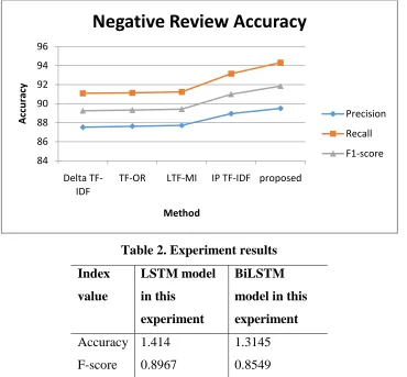
IP TF-IDF 92.82 88.40 90.55 88.94 93.15 90.99

proposed 93.6 90.2 91.87 89.5 94.32 91.85

82 84 86 88 90 92 94 96

Delta TF-IDF

TF-OR LTF-MI IP TF-IDF proposed

A

cc

u

rac

y

Method

Positive Review Accuracy

Precision

Recall

(24)

Table 2. Experiment results

Index

value

LSTM model

in this

experiment

BiLSTM

model in this

experiment

Accuracy 1.414 1.3145

F-score 0.8967 0.8549

The experiment results are compared with those of Tang et al., as shown in Table 3.

Table.3. Result comparison

Index

value

LSTM model BiLSTM model

Present

study

Existing

study

Present

study

Existing

study

Accuracy 1.3653 0.9074 1.1567 0.9089

F-score 0.9843 0.6547 0.7980 0.6770 84

86 88 90 92 94 96

Delta TF-IDF

TF-OR LTF-MI IP TF-IDF proposed

A

cc

u

rac

y

Method

Negative Review Accuracy

Precision

Recall

(25)

In this paper, an improved RNN language model is put forward ü LSTM, which

successfully covers all history sequence information and performs better than conventional RNN.

It is applied to achieve multi-classification for text emotional attributes, and identifies text

emotional attributes more accurately than the conventional RNN.

For RNN model, scientists put forward an idea named „Attention‟ which may lead to

better results. This is to make RNN select information from larger information set in each step.

Besides, „Attention‟ is not the only development in RNN area. Scientists have proposed Grid

LSTM which also showed excellent performances in some application scenarios. In future work,

we could try these improvement programs or use different models combination to improve the

performance of text sentiment analysis.

In this paper, in order to verify the performance of our method, a widely used standard

dataset is selected as the experimental dataset. The dataset, ChnSentiCorp_htl_ba_4000. In this

paper, it is called the Chinese hotel dataset. The dataset contains 4000 documents (2000 negative

and 2000 positive).

According to the data comparison in Table 3, the performance of the improved BiLSTM

model in Chinese is better than that of the original LSTM. The use of the BiLSTM to model the

text in two directions slightly influenced the judgment of the emotional polarity of the features.

The reason may be that the LSTM model has a memory function on the context; consequently,

the relative position of the text input has no effect on the model, and its absolute position is the

key factor that affects the model. From the experimental results, the application of the LSTM 0

0.2 0.4 0.6 0.8 1 1.2

LSTM BILSTM SVM model ELM-LSTM

A

cc

u

rac

y

Method

Accuracy

(26)

(IJARSE) 2012, Vol. No.1, Issue No. 8, August ISSN-2319-8354 model to the Chinese language achieved good results after a series of modifications to Chinese

characters was made. In comparison with the results of Tang et al. in English, accuracy and

F-scores in Chinese improved, which indicates that the LSTM model is effective in Chinese

fine-grained sentiment analysis. The use of the LSTM network in finefine-grained sentiment analysis of

Chinese customer reviews is feasible and effective. As shown in Figure 7, the performance of the

sentiment analysis of the LSTM model is greatly enhanced, compared with the traditional

learning model, because the use of LSTM networks for sentiment analysis of product features

does not require priori knowledge, such as syntactic parsing or sentiment lexicon. Only the

LSTM model is used to consider the effect of context on feature emotional polarity. The

emotional polarity in product features is judged automatically. Moreover, the LSTM model has

long-term memory to the context of reviews text, which makes up for the disadvantage of the

traditional sentiment ansalysis of neglecting product feature text context, which makes the

judgment of emotional tendency on product features more accurate.

Overall, we achieved a satisfactory accuracy score of 63% using the LSTM-CNN model

compared to a baseline model which used Naïve Bayes as a classifier. The experiment showed

the ability of the CNN to act as powerful feature extractors and LSTM to capture changing

sentiment in a long text.

Conclusion

We propose an improved term weighting scheme in this paper, which combines the

contribution of feature terms to the class, the local distribution in the document, and the global

distribution in the document set. Compared with a series of weighted schemes, experimental

results on a widely used Chinese dataset verify that the proposed scheme is effective and can

significantly improve the classification performance. In the future, we plan to combine our

scheme with other feature selection methods that reflect class distinctions and verify their

effectiveness on more datasets which belong to different domains that aims to gain a better

classification performance. Finally, the performance of the proposed scheme on unbalanced

corpus is also the focus of the followup work.

References

[1] Jithin, “Text Classification Using KM-ELM Classifier “, 2016 International Conference on Circuit,

Power and Computing Technologies [ICCPCT].

[2] Shah, “Clustering Based Feature Selection using Extreme Learning Machines for Text Classification

(27)

(IJARSE) 2012, Vol. No.1, Issue No. 8, August ISSN-2319-8354 [3] Yong, “Multi-document Extractive Summarization Using Window-based Sentence Representation “,

2015 IEEE Symposium Series on Computational Intelligence.

[4] Pranav, “A New Feature Selection Technique Combined with ELM Feature Space for Text

Classification “.

[5] Philip, “Regularized Training of the Extreme Learning Machine using the Conjugate Gradient

Method “, School of Electrical and Information Engineering.

[6] Azreen, “Improvement of Sentiment Analysis based on Clustering of Word2Vec Features “, 2017

28th International Workshop on Database and Expert Systems Applications.

[7] Sathish, “Concept detection and Cluster Analysis from Newsfeed- Singular value decomposition

based Approach “, 2016 International Conference on Computational Intelligence and Networks.

[8] XU YUAN, “Semantic Clustering-Based Deep Hypergraph Model for Online Reviews Semantic

Classification in Cyber-Physical-Social Systems “, School of Software, Dalian University of

Technology, Dalian, China.

[9] Emil, “Unsupervised Aspect Level Sentiment Analysis Using Ant Clustering and Self-organizing

Maps “, Technical University of Cluj-Napoca.

[10] Shuanglu, “Integrating Visual and Textual Affective Descriptors for Sentiment Analysis of Social

Media Posts “, 2018 IEEE Conference on Multimedia Information Processing and Retrieval

[11] Tao Wang,” Reasearch on Feature Mapping Based on Labels Information in Multi-label Text

Classification “, Beijing University of Posts and Telecommunications.

[12] Gargi, “Unsupervised Classification of Online Community Input to Advance Transportation Services

“Department of Computer Science.

[13] AsliCelikyilmaz, “An Empirical Investigation of Word Class-Based Features for Natural Language Understanding “, IEEE/ACM Transactions on Audio, Speech, and Language Processing.

[14] Amir Hamzah, “Opinion Classification Using Maximum Entropy and K-Means Clustering “,2016

International Conference on Information, Communication Technology and System (ICTS).

[15] Jyoti, “Text Classification using Semi-supervised Approach for Multi Domain “,2017 International