Available Online at www.ijcsmc.com
International Journal of Computer Science and Mobile Computing
A Monthly Journal of Computer Science and Information Technology
ISSN 2320–088X
IJCSMC, Vol. 4, Issue. 5, May 2015, pg.736 – 740
RESEARCH ARTICLE
An Improved Random Forest Algorithm for
Prediction of Protein-Protein Interaction
Tung Thanh Pham
1¹
Information Technology Department, Ho Chi Minh City University of Foreign Languages and Information Technology, Viet Nam1
Abstract— Protein-protein interaction (PPI) is a combining two or more protein because of biochemical events in any living cell. Protein domains are functional and/or structure units in a protein and consequently they are responsible for protein-protein interaction. Many machine-learning approaches with domain-based models for protein interaction prediction and their feasibility are showed. In this study, we developed a domain-based predictor based on Random Forest (RF) algorithm with the CPRS method, it is based on cost proportional roulette sampling technique and create training sample in constructing ―forest‖. Moreover, the paper applied the theory ―A protein pair is interaction with each other when they are the same function and position‖. Experimental results on Saccharomyces cerevisiae dataset show that our protein–protein interactions predictor has higher than some model with sensitivity (81.7%) and specificity (73.6%).
Keywords— Random Forest, Protein-protein interaction, Domain, Roulette Sampling Technique
I. INTRODUCTION
Proteins play an essential role in nearly all biological events and cell functions by interacting with other proteins. The variety of functions is attributed to the interactions with other proteins. Understanding the characteristics of PPIs is critical. The high throughput methods such as Yeast 2-Hybrid (Y2H) and mass spectrometry methods help determine protein interactions. Through these methods suffer from high false positive rates, we need to find additional in computational methods that are the more accurately predicting interactions.
A number of machine learning approaches for protein interaction have been proposed over the years. The method demonstrate the feasibility such as Bayesian classifier, Random Forest, Logistic Regression, Support Vector Machines and Decision Tree. They apply the indirect information from Gene Ontology annotation, gene expression correlation, sequence homology etc. to predict PPI.
Recently, much domain-based method is interest. Domains are a part of protein sequence and structure that can evolve, function, and exist independently of the rest of the protein chain. And we assume that proteins interact with each other as a result of the combination of their domains.
There are many different approaches in data classification of PPI. The current methods can be divided into two classes:
1) Single-domain interaction [4] [5] 2) Multi-domain interaction: [1] [3].
II. METHODS
A. Feature representation
The solving of PPI prediction problem is the binary classification problem (two-label): each sample is a protein pair, it is assigned „interaction‟ label (this is the interaction proteins pair) or „non-interaction‟ label (the protein pair do not interact). In our approach, a protein pair is represented by the domains existing in each protein. In our database (training and testing dataset), we use 4293 unique Pfam domains. Thus, each sample is a vector of 4293 features in which a feature is a domain. Let
D
X X
1,
2, ,
X
N
denote the N training samplesand
1 , 2 , , 4293,
i i i
i i
X x x x y is the i-th sample with 4293 feature attributes, xj belonging to the label yi. In
our problem, yi = 1 correspond to the „interaction‟ class and 0 to the „non-interaction‟ class. Each feature xj has
a discrete value of 0, 1 or 2. The feature value is 0 that mean the protein pair does not contain the domain. The value is 1 as the domain belong one protein of the pair. Finally, the proteins pair has the domain, then it is 2. Training decision trees with a binary-valued feature is faster than that with a ternary-valued feature, but a binary-valued feature may not be able to show protein pairs with a domain existing in one protein and those with the domain existing in both proteins.
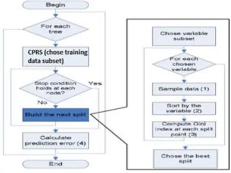
Figure 1 Our random forest algorithm
B. Random decision forest
Random Forests grows many classification trees and is announced by Breiman in 2001. Each tree is constructed as follows:
If the number of sample in the training set is N, sample N cases at random - but with replacement, from the original data.
If there are M input variables (feature), a number m<<M is specified such that at each node, m variables are selected at random out of the M and the best split on these m is used to split the node. The value of m is held constant during the forest growing.
Each tree is grown to the largest extent possible. There is no pruning
When we classify a new object, each classification tree in the forest gives a label which is denoted as the tree „voting‟ for that label. Majority votes among the label decided by the forest of trees that the object receive as the result of classification.
The forest error rate depends on correlation and strength. The correlation between any two trees in the forest, increasing the correlation increases the forest error rate. The strength of each tree in the forest. A tree with a low error rate is a strong classifier. Increasing the strength of the individual trees decreases the forest error rate. The parameter m (m feature is used to constructing decision tree). Reducing m reduces both the correlation and the strength. Increasing it increases both. In the particular problem, the m-parameter must be optimized. The out-of-bag error estimate is normally used to finding a value of m.
C. Cost Proportionate Roulette Sampling (CPRS)
For binary classes, we assume we have the misclassification costs false positive (FP, the cost of misclassifying a negative instance into positive) and false negative (FN, the cost of misclassifying a positive instance into negative), and the cost of correct classification is zero. We simply assign FP as the weight to each negative instance, and assign FN as the weight to each positive instance. That is, the weight ratio of a positive instance to a negative instance is proportional to FN/FP [2].
In the cost proportional roulette sampling, we normalize their weights such that the sum of them equals to the number of instances. If we have a training set with P positive instances and N negative instances, then the
weight of each negative instance is FP
P N
P FN N FP
, and the weight of each positive instance is
FN P NP FN N FP
.
Thus, the sum of the weights is P+N. That is, the length of the mapped line is P+N. One of the important steps of roulette sampling is to select an example. Each time, roulette sampling generates a random number within the range of the length of the line. Then the example whose segment spans the random number is selected. The selection process does not stop until the total number of examples is reached. That is, users can indicate the size of samples generated by roulette sampling.
Like rejection sampling, roulette sampling makes use of the misclassification cost information. However, unlike rejection sampling, which draws examples independently from the distribution of the original training set, roulette sampling takes the distribution of original training set into consideration. In sum, roulette sampling integrates the effect of misclassification cost, the distribution of original training set, and the size of samples.
D. Our domain-based predictor
Our predictor is the same standard random forest algorithm; each tree in the random forest is created from a dataset that is selected from training data by CPRS method. That is, we repeatedly perform cost proportional roulette sampling to generate multiple set from the original training set, and learn a tree from each sampled. The random forest selects randomly a feature subset at each splitting node when building a decision tree.
At each level of decision tree, the „goodness of split‟ measure is the information gain. It measures the theoretical information content of a code by log
i i
i
p p
, where pi is the probability of the i-thmessage.In our random forest, trees are pruned when it completely built. We use a stopping criterion when all samples are classified. This is a stops splitting node in a decision tree when any of the following conditions is met: a number of node in tree reach the maximum, node impurity is smaller or equal to the threshold, or number of the remained samples is minimum.
When a random forest classify a protein pair that receive a label, that means that all most decision tree of forest classify same label for the pair. Moreover, votes are accepted if the trees that contain at least one domain feature from each protein of the pair at splitting node. The requirement must be quarantined, because decision tree do not contain domains from a protein pair that will not denote the proteins interact with each other. In my approach, we specify a number of tree that cover covers each domain feature in the training samples. A tree is not able to vote for a protein pair, the protein pair is non-interacting.
III.EXPERIMENTAL RESULTS
A. Data sources
Initially, our dataset have 9834 interaction pairs with 3713 proteins, and it is split with two part. Each part have 4917 pairs into training and testing datasets [1] [4]. So non-interacting data are not available, the protein pair are randomly generated. The generation is based on a theory “A protein pair is interaction with each other when they are the same function and position”. Hence, the two proteins do not interact with each other when they are not at the same position and/or function. Further, a sample is considered to be a negative sample if it does not belong to the interaction set. The functions and positions of protein is extracted from UniProt database [9] and Saccharomyces Genome Database [7]. The negative dataset were randomly made with the above theory and there are 8000 negative protein pairs. We also divided into two subset (negative training and testing subset). The final training and testing datasets have 8917 samples, 4917 positive and 4000 negative samples.
B. Evaluation measures
We evaluate the prediction PPIs with specificity and sensitivity parameters. The specificity SP is defined as the percentage of matched non-interactions between the predicted set and the observed set over the total number of observed non-interactions. The sensitivity, denoted by SN, is defined as the percentage of matched interactions over the total number of observed interactions [1].
C. CPRS’s parameters
In this section, the cost of false positive (FP) and false negative (FN) were obtained from [3]. FN =1.05, FP = 0.95 and FN = 1.25, FP = 0.9; P=4917, N=4000.
D. Predicting PPI
In our implementation, there are three stopping criteria: maximum tree node, impurity and minimum node size thresholds. Minimum node size is the minimum number of samples to be classified by each node. In our forest, each decision tree is constructed with node impurity threshold of 0.01, and the minimum number of samples at a node is three. The stopping criteria was applied when <10% reached impurity and minimum node size thresholds. The maximum tree node has the most impact in restricting the tree size. Thus, we grow forests of trees with different heights to make an appropriate parameter choice on maximum tree level threshold. We used 10-fold cross-validation and found that classification error rates over the validation sets decrease first as the tree levels increase. This is due to the increased performance of each individual tree. Because of majority voting, if each individual tree in a forest performs better, then the entire forest will also perform better.
To determine an appropriate number of trees in a forest, we set a limit on minimum coverage of each domain feature at 30 trees. In other words, it makes sure that each domain feature appeared in the training dataset is one of splitting attributes in at least 30 trees. In this way, we guarantee that at least a certain number of trees will vote to classify each protein pair. From the experiment, we found that with 100 trees in the forest, at least 74 trees cover each domain feature.
The result of our method is compared with the Chen et al., 2005 results. In their paper, different values of the false positive and false negative rates are evaluated. Table 1 shows the best results of our method and [5] over the test dataset.
TABLEI
ACCURACY COMPARISON: OUR BEST METHOD AND CHEN ET AL.2005
Our Method Chen et al. 2005
Sensitivity (SN) 81.7% 79.8%
Specificity (SP) 73.6% 64.4%
TABLEIII
ACCURACY COMPARISON: OUR METHOD (FN=1.05,FP=0.95 AND FN=1.25,FP=0.9)
FN=1.05, FP = 0.95 FN=1.25, FP = 0.9
Sensitivity (SN) 81.7% 84.5%
Specificity (SP) 73.6% 70.3%
TABLEIIIII
ACCURACY COMPARISON: OUR RANDOM FOREST AND SVM
Our Random Forest SVM[6]
Sensitivity (SN) 81.7% 81.8%
Specificity (SP) 73.6% 77.5%
IV.CONCLUSIONS
REFERENCES
[1] X.-W. Chen and M. Liu, Prediction of Protein–Protein Interactions Using Random Decision Forest Framework, Bioinformatics, vol. 21, pp. 4394–4400. Oct 2005.
[2] C. X. Ling and V. S. Sheng, “Roulette Sampling for Cost-Sensitive Learning”, in Proc. ECML 2007, LNAI 4701, pp.724-731.
[3] [3] W. Gou, Y. Hu, M. Liu, J. Yin, K. Xie and Y. Xiaobo, “Exploring CostSensitive Learning in Domain Based Protein-Protein Interaction Prediction”, in Proc. ISNN 2009, AISC 56, pp 175-184.
[4] Kim,W.K.et al., Large scale statistical prediction of protein–protein interaction, Genome Inform. Ser. Workshop Genome Inform, 13, pp. 42-50, 2002.
[5] Qi,Y.et al, Random forest similarity for protein–protein interaction prediction from multiple sources, Pac. Symp. Biocomput., pp. 531-542, 2005.
[6] R.-E. Fan, K.-W. Chang, C.-J. Hsieh, X.-R. Wang and C.-J. Lin (2008), "LIBLINEAR: A Library for Large Linear Classification, Journal of Machine Learning Research, vol. 9, pp. 1871-1874.