8- BAND HYPER-SPECTRAL IMAGE COMPRESSION USING EMBEDDED ZERO TREE WAVELET

8- BAND HYPER-SPECTRAL IMAGE COMPRESSION

USING EMBEDDED ZERO TREE WAVELET

Harshit Kansal

1

, Vikas Kumar

2

, Santosh Kumar

3

1

Department of Electronics & Communication Engineering, BTKIT, Dwarahat-263653(India)

2,3

Department of Electronics & Communication Engineering, INVERTIS University, Bareilly (India)

ABSTRACT

Hyperspectral imaging is a powerful technique and has been widely used in a large number of applications,

such as detection and identification of the surface and atmospheric constituents present, analysis of soil type,

monitoring agriculture and forest status, environmental studies, and military surveillance. It consumes a huge

amount of storage. So due to large memory requirements, Hyper-spectral images demand efficient compression.

The Hyper-spectral image which we have taken in this paper is the Moffett field image which is taken by

Airborne Visible Infra Red Imaging Spectrometer (AVIRIS) satellite. In this paper we have presented an

algorithm which adapts EZWfor quantization, Wavelet Transform for decorrelation and Entropy coding is done

by Adaptive Arithmetic Coding. The results obtained show the efficient compression and are comparable to

JPEG 2000 standard.

Keywords: Hyper-Spectral Images, Embedded Zero Tree Wavelet (EZW), Discrete Wavelet

Transform (DWT), Arithmetic Coding

I INTRODUCTION

Hyperspectral images are generated by collecting hundreds of narrow and contiguously spaced spectral bands of

data such that a complete reflectance spectrum can be obtained for the region being viewed by the instrument.

All substances, including living things, have their own spectrum characteristics or diagnostic absorption

features.

However, at the time we gain high resolution spectrum information, we generate massively large image data

sets. Access and transport of these data sets will stress existing processing, storage and transmission capabilities.

As an example, the Airborne Visible Infra Red Imaging Spectrometer (AVIRIS), a typical hyperspectral

imaging system, has 224 sensors. In order to provide sufficient resolution to detect most absorption features,

each sensor has a wavelength sensitive range of approximately 10 nanometers. All sensors together yield

contiguous spectral bands covering the entire range between 380 nm and 2500 nm. If each band is 614 × 512

scans (pixels), with one byte per pixel, the whole data set will be over 70 Mbytes. Actually, AVIRIS instrument

can yield about 16 Gigabytes of data per day. Therefore, efficient compression should be applied to these data

sets before storage and transmission.Obviously, the low compression ratio is not enough to cope with serious

information, we can gain significantly higher compression ratio than that of lossless compression. This is

so-called lossy compression (lossy coding).

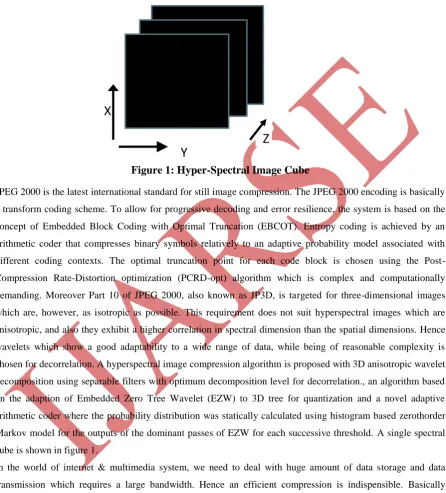
Figure 1: Hyper-Spectral Image Cube

JPEG 2000 is the latest international standard for still image compression. The JPEG 2000 encoding is basically

a transform coding scheme. To allow for progressive decoding and error resilience, the system is based on the

concept of Embedded Block Coding with Optimal Truncation (EBCOT). Entropy coding is achieved by an

arithmetic coder that compresses binary symbols relatively to an adaptive probability model associated with

different coding contexts. The optimal truncation point for each code block is chosen using the

Post-Compression Rate-Distortion optimization (PCRD-opt) algorithm which is complex and computationally

demanding. Moreover Part 10 of JPEG 2000, also known as JP3D, is targeted for three-dimensional images

which are, however, as isotropic as possible. This requirement does not suit hyperspectral images which are

anisotropic, and also they exhibit a higher correlation in spectral dimension than the spatial dimensions. Hence

wavelets which show a good adaptability to a wide range of data, while being of reasonable complexity is

chosen for decorrelation. A hyperspectral image compression algorithm is proposed with 3D anisotropic wavelet

decomposition using separable filters with optimum decomposition level for decorrelation., an algorithm based

on the adaption of Embedded Zero Tree Wavelet (EZW) to 3D tree for quantization and a novel adaptive

arithmetic coder where the probability distribution was statically calculated using histogram based zerothorder

Markov model for the outputs of the dominant passes of EZW for each successive threshold. A single spectral

cube is shown in figure 1.

In the world of internet & multimedia system, we need to deal with huge amount of data storage and data

transmission which requires a large bandwidth. Hence an efficient compression is indispensible. Basically

compression consists of three steps: Decorrelation, Quantization & Entropy coding. Decorrelation is the step to

remove the inter-pixel dependencies in image data.Quantization can be done by EZW or its variants. Entropy

coding removes the redundancies due togrey level distribution in decorrelated image.In this proposed work we

have chosen 3D Wavelet decomposition. For quantization we have used 3D Embedded Zero Tree coding of

Wavelet coefficients. Entropy coding is done by Adaptive Arithmetic coding.

X

Wavelet functions are used to analyze the difference subspaces and are represented as

ψ

r,s

(x) = 2

r/2

ψ(2

r

x-s)

(1)

where r = scaling parameter

s = shift parameter

x = continuous time variable

A Wavelet function can be analyzed by using the summation of shifted versions of scaling functions of next

higher subspace. Mathematically it is represented as

ψ(x) =

𝒉

𝒏 _𝜳

𝒏 𝟐𝜱(𝟐𝒙 − 𝒏)

(2)

where n = shift parameter

Φ = scaling function

hψ= coefficient

The main advantage of using Wavelet Transform is that it gives us the space frequency localization. i.e. which

frequency is present at which position. It is similar to pin-pointed short time Fourier Transform. Forward

Discrete Wavelet Transform (DWT) is represented as

W

Φ

(

𝒋

𝟎

,k) =

𝟏

𝑴

𝒔 𝒏 𝜱

𝒏 𝒋𝟎,𝒌

(𝒏)

(3)

W

ψ

( j, k) =

𝟏

𝑴

𝒔 𝒏 𝜱

𝒏 𝒋,𝒌

(𝒏)

(4)

Where ( j> j0)

Here

W

Φ

(

𝑗

0

, k)

=

scaling function coefficient

W

ψ

( j, k)=

Wavelet function coefficient

j = scaling parameter

k = shift parameter

s(n) = Discrete-time signal

for n = 0,1…..M-1.

For reconstruction of signal back from the two coefficient is done by Inverse DWT as shown

S (n) =

𝟏

𝑴

𝑾

𝒌 𝜱

𝒋

𝟎

, 𝒌 𝜱

𝒋𝟎,𝒌

𝒏 +

𝟏

𝑴

𝑾

𝒌 𝝍

𝒋, 𝒌 𝝍

𝒋,𝒌

(𝒏)

∞

𝒋=𝒋𝟎

(5)

From above equations it can be analyzed that

W

ϕ

(j,k) =

𝒉

𝒌 𝝓

𝒎 − 𝟐𝒑 𝑾

𝝓

𝒋 + 𝟏, 𝒌

(7)

The above equation shows that DWT uses two filters with impulse responses

ℎ

_𝜙 (scaling analysis filter)

&

ℎ

_𝜓(Wavelet analysis filter) with input as original signal [𝑊𝜙(𝑗 + 1, 𝑘)]. Figure 2 shows the Block diagram of this filter bank.

FIGURE 2: 1-Level Decomposition Using Filter Bank

II IMAGE COMPRESSION

Compression can be classified as lossless &lossy compression. As the name suggests that in Lossless

compression, we do not lose any in information and can reconstruct the original signal. But this type of

compression does not provide an effective compression ratio. If we can compromise with some part of

information to be loosed then a lossy compression is a better choice. Basically there are three kinds of

redundancies in 2D data: Coding Redundancy, Spatial and Temporal Redundancy & Irrelevant information.

Thus compression is a step to remove one of these redundancies. There are many standards for image

compression. Although Joint Photographic Evaluation Group (JPEG) is a Lossy compression but it uses DCT

for decorrelation and run-length coding or Huffman coding for Entropy coding. So we could use JPEG2000

which use Arithmetic coding & DWT. JPEG2000 gives a better quality of compression for photographic

images. The part 10 of JPEG2000, also known as JP3D, is targeted for 3D images which are as isotropic as

possible. So it does not suit to Hyper-spectral image compression. The paper shows an alternative but less

complex approach for these type of compression.

2.1 Dyadic Wavelet Decomposition

As Wavelet filters are separable filters so we have applied 1D Wavelet transform in all the dimensions.

Although we could apply non-separable filter but it is harder to design such a filter. For a 2D signal [s(𝑛1, 𝑛2)] we get a bank of filters responses as below:

ϕ

(𝒏

𝟏

, 𝒏

𝟐

) = ϕ(

𝒏

𝟏

) ϕ(

𝒏

𝟐

)

(8)

𝝍

𝑯

𝒏

𝟏

, 𝒏

𝟐

= 𝝍 𝒏

𝟏

ϕ(

𝒏

𝟐

)

(9)

𝝍

𝒓

𝒏

𝟏

, 𝒏

𝟐

= 𝛟 𝒏

𝟏

𝝍 𝒏

𝟐

(10)

𝝍

𝑫

_𝒏

𝟏

, 𝒏

𝟐

= 𝝍 𝒏

𝟏

𝝍

(

𝒏

𝟐

)

(11)

ℎ

𝜙

(−𝑛)

ℎ

𝜓

(−𝑛)

↓ 2

↓ 2

𝑊𝜙(𝑗 + 1, 𝑘)

W

ϕ

(j,k)

Where

ϕ(𝑛1, 𝑛2) represents the signal Low-pass filtered along the row & along the column.[LL]

𝜓𝐻 _𝑛

1, 𝑛2 represents the signal High-pass filtered along the row & Low-pass filtered along the column.[HL]

𝜓𝑟 _𝑛

1, 𝑛2 represents the signal Low-pass filtered along the row & High-pass filtered along the column.[LH]

𝜓𝐷 _𝑛

1, 𝑛2 represents the signal High-pass filtered along the row & along the column. [HH] The individual filter responses can be represented individually as in figure 3.

LL

HL

LH

HH

Figure 3: 1-Level Decomposition Of 2d Signal

The Low-pass filtered signal is very rich in information. So further decomposition on LL sub-band is done. The

2-level decomposition is shown in figure 4.

LL

2

HL

2

HL

1

LH

2

HH

2

LH

1

HH

1

Figure 4: 2-Level Decomposition Of 2d Signal

This process of decomposition is known as Dyadic Decomposition. It is to be decided upto which level we

should go.

2.2 Zero Tree Coding Of Wavelet Coefficients

Zero tree provides a multi-resolution representation of Significant Map indicating the position of Significant

coefficients. It allows the successful prediction of insignificant coefficients. Successive approximation provides

the compact representation of significant coefficients & facilitates embedding algorithm. Larger coefficients are

more important than smaller one regardless of their scale. The algorithm runs in recursive manner until the

required bit rate is not achieved. Figure 5 shows the flow chart for encoding the Wavelet coefficients in Zero

Figure 5: Flow Chart for Encoding Wavelet coefficients

2.3 Adaptive Arithmetic Coding

Arithmetic Coding is a lossless data compression technique. It encodes the data into the form of a string that

represents a fractional value between 0 &1. The bit stream from subordinate pass of Zero Tree coding is hardly

to compress. So these are outputted as they are. Arithmetic coding is performed only on the string coded from

dominant pass. Probability of each letter in coded string is calculated statically. In case of remote sensing

applications where huge amount of data have to be transmitted, higher coding speed is an essential requirement.

The proposed scheme gives a higher bit rate saving than any memory less model.

2.4 Compression with Proposed Algorithm

The Algorithm for Image compression of Hyper-spectral images is as follows:

1. Download the data file (Moffett Field) from NASA website.

2. Rearrange the data in bit interleaved per pixel (bip) format.

3. Implement a 2D image compression coder using Adaptive Arithmetic coding in MATLAB.

4. Check the efficiency of Adaptive Arithmetic coder.

5. Decide the value for decomposition level & filter type using 2D results.

6. Develop a Hyper-spectral image compression algorithm with Adaptive Arithmetic coding in

7. A file size of 614x512x224x2 is arranged in the size of 512x512 with 8 bands.

8. Design a graph for BPP versus PSNR.

III PERFORMANCE MEASURES

The best way to check any signal with the original one is the difference between two signals. The two popular

measures are squared error measure & absolute difference measure. If the two signals are x(n) & y(n) then

squared error is given by

p(x, y) = (x - y)

2

(12)

And the absolute error is given by

q(x, y) = |x – y|

(13)

It is difficult to find the difference between the two on the term basis. So we go for Mean Square error (MSE) &

it is represented by σ2_.

σ

2

=

_𝑵𝟏 𝑵𝒏=𝟏 𝒙𝒏−𝒚𝒏 𝟐

(14)

If we are interested in size of error relative to the original signal then we can calculate the ratio of the average

squared value of original signal to the MSE i.e Signal to Noise ratio (SNR).

SNR =

𝝈𝒙

𝟐

𝝈𝟐

(15)

Where

𝜎

_𝑥2is the average squared value of original signal.SNR is often measured in decibels (dB).

SNR (dB) =10

𝐥𝐨𝐠

𝟏𝟎 𝝈𝒙𝟐

𝝈𝟐

(16)

Sometimes we are more interested in peak value then we go for Peak Signal to Noise Ratio (PSNR).

PSNR (dB) = 10

𝐥𝐨𝐠

𝟏𝟎 𝝈_{𝒙𝒑𝒆𝒂𝒌}𝟐

𝝈𝟐

(17)

IV EXPERIMENTAL RESULTS

An algorithm was developed using 2D wavelet transform for decorrelation, 2D EZW for quantization and

Huffman coding for entropy coding. The decision of filter choice & decomposition level is done by applying 2D

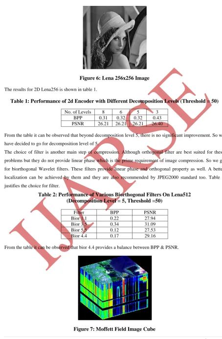
Figure 6: Lena 256x256 Image

The results for 2D Lena256 is shown in table 1.

Table 1: Performance of 2d Encoder with Different Decomposition Levels (Threshold = 50)

No. of Levels 8 6 5 3 BPP 0.31 0.32 0.32 0.43 PSNR 26.21 26.21 26.21 26.40

From the table it can be observed that beyond decomposition level 5, there is no significant improvement. So we

have decided to go for decomposition level of 5.

The choice of filter is another main step of compression. Although orthogonal filter are best suited for these

problems but they do not provide linear phase which is the prime requirement of image compression. So we go

for biorthogonal Wavelet filters. These filters provide linear phase and orthogonal property as well. A better

localization can be achieved by them and they are also recommended by JPEG2000 standard too. Table 2

justifies the choice for filter.

Table 2: Performance of Various Biorthogonal Filters On Lena512

(Decomposition Level = 5, Threshold =50)

Filter BPP PSNR

Bior 1.1 0.22 27.94

Bior 3.5 0.34 31.09

Bior 5.5 0.12 27.53

Bior 4.4 0.17 29.16

From the table it can be observed that bior 4.4 provides a balance between BPP & PSNR.

The objective is to evolve a Hyper-spectral image compression, which is less complex & also provides a better

performance. The test data for 3D image compression is the scene of Moffett field, California, at south end of

San Francisco Bay imaged by AVIRIS. The data is in Bit interleaved per pixel (bip) format. The result obtained

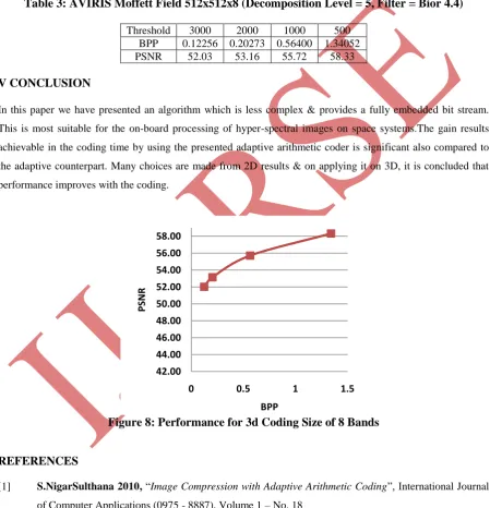
for spatial dimension of 512x512 with band size of 8 is tabulated in Table 3. The graph drawn from the data

shows that as coding size increases performance increases too. So as the Bit per pixel values increases PSNR

also increases.

Table 3: AVIRIS Moffett Field 512x512x8 (Decomposition Level = 5, Filter = Bior 4.4)

Threshold 3000 2000 1000 500 BPP 0.12256 0.20273 0.56400 1.34052 PSNR 52.03 53.16 55.72 58.33

V CONCLUSION

In this paper we have presented an algorithm which is less complex & provides a fully embedded bit stream.

This is most suitable for the on-board processing of hyper-spectral images on space systems.The gain results

achievable in the coding time by using the presented adaptive arithmetic coder is significant also compared to

the adaptive counterpart. Many choices are made from 2D results & on applying it on 3D, it is concluded that

performance improves with the coding.

Figure 8: Performance for 3d Coding Size of 8 Bands

REFERENCES

[1] S.NigarSulthana 2010, “Image Compression with Adaptive Arithmetic Coding”, International Journal

of Computer Applications (0975 - 8887), Volume 1 – No. 18

[2] J.M. Shapiro 1993 “Embedded image coding using zerotrees of wavelet coefficients,” IEEE

Transactions on signal processing, vol.41, no.12, pp.3445-3462

[3] A. Said 2004, “Introduction to Arithmetic Coding-Theory and Practice”, Imaging Systems Laboratory,

HP Laboratories Palo Alto, HPL-2004-76

42.00 44.00 46.00 48.00 50.00 52.00 54.00 56.00 58.00

0 0.5 1 1.5

PS

N

R

[4] E. Christophe 2011, “Hyperspectral Data Compression Tradeoff”, Centre for Remote Imaging,

Sensing and Processing, National University of Singapore, Singapore.

[5] http://aviris.jpl.nasa.gov

[6] E. Christophe, C.Mailhes, and Pierre Duhamel 2008, “Hyperspectral Image Compression: Adapting

SPIHT and EZW to Anisotropic 3-D Wavelet Coding”, IEEE Transactions on Image Processing, vol.

17, no. 12

[7] Alessandro J. S. Dutra 2010, “Successive Approximation Wavelet Coding of AVIRIS Hyperspectral

Images” CIPR Technical Report TR-2010-3

[8] B.E.Usevitch 2001, “A Tutorial on Modern Lossy wavelet image compression: Foundations of JPEG

2000,” IEEE Transactions on signal processing

[9] Barbara Penna 2005, “Embedded lossy to lossless compression of hyperspectral images using JPEG

2000”, Center for Multimedia Radio Communications, IEEE