Machines
?Sanjam Garg and Akshayaram Srinivasan University of California, Berkeley {sanjamg,akshayaram}@berkeley.edu
Abstract. We give a simple construction of indistinguishability obfus-cation for Turing machines where the time to obfuscate grows only with the description size of the machine and otherwise, independent of the running time and the space used. While this result is already known [Koppula, Lewko, and Waters, STOC 2015] from iO for circuits and injective pseudorandom generators, our construction and its analysis are conceptually much simpler. In particular, the main technical com-ponent in the proof of our construction is a simple combinatorial peb-bling argument [Garg and Srinivasan, EUROCRYPT 2018]. Our con-struction makes use of indistinguishability obfuscation for circuits and somewhere statistically binding hash functions.
1
Introduction
Indistinguishability Obfuscation (iO) [BGI+12, GGH+13] is a central
primi-tive in cryptography giving rise to new and powerful cryptographic applica-tions [SW14, GGHR14].iO requires that for any two circuitsC0 andC1 com-puting the exact same functionality, obfuscation of C0 is computationally in-distinguishable from the obfuscation ofC1. While circuits are powerful enough
to simulate other models of computation such as Turing machines or RAM pro-grams [PF79], a drawback of using them is that size of the circuit (and hence the size of obfuscation) grows with both the running time and the space of the com-putation. In a beautiful work Koppula, Lewko and Waters [KLW15] (building on prior work [BGL+15, CHJV15]) showed a method for removing this
limita-tion by giving a construclimita-tion of succinct iO for Turing machines from iO for circuits and injective pseudorandom generators. By succinct, we mean that the time to obfuscate a machine grows only with its description size and is otherwise independent of its running time and its space complexity.
Our Contribution.In this paper, we give asimpleconstruction of succinct in-distinguishability obfuscation for Turing machines from sub-exponentially secure ?Research supported in part from 2017 AFOSR YIP Award, DARPA/ARL
iOfor circuits and sub-exponentially secure somewhere statistically binding hash functions [HW15, KLW15]. Our new construction is simple to describe and its analysis is
much simpler than the previous works. Inspired by [GS18a], the main technical component in our security proof is a simple combinatorial pebbling argument.
In a bit more detail, we achieve the above new result by first giving a new con-struction of succinct randomized encoding [AIK04, CHJV15, BGL+15, App17] from polynomially hard indistinguishability obfuscation for circuits and laconic oblivious transfer [CDG+17, DG17, BLSV18, DGHM18].1 A randomized encod-ing allows to encode a Turencod-ing machine M, an input xand a time bound t to
c
Mx,t. Given Mcx,t, the decoding procedure recovers M(x) which is the output of M on input x obtained in time t. The security property requires that the distribution ofMcx,tdoes not leak anything aboutxexceptM(x). A randomized encoding is said to be succinct if the encoding procedure runs in time that is polynomial in the security parameter, the machine description size and the input size and is otherwise independent of the time and space complexity ofM. Next, to construct succinctiOfor Turing machines, we use a transformation from any succinct randomized encoding (with sub-exponential security) to succinct iO for Turing machines given in the works of [CHJV15, BGL+15]. This yields the
desired result.
1.1 Overview
In this section, we give a high level overview of our construction of succinct randomized encodings and the security proof.
Starting point. The starting point of our work is the construction of semi-succinctrandomized encodings for Turing machines in [CHJV15, BGL+15] based
oniOfor circuits and Yao’s garbling scheme. Semi-succinct randomized encod-ings require that the time to encode a machine to be independent of its running time but could depend on the space complexity of the computation. In partic-ular, it is a weaker requirement when compared to full succinctness wherein we also require the time to encode a machine to be independent of the space com-plexity. Below we start by recalling this construction and explain why it achieves only semi-succinctness when compared to full succinctness.
The encoding procedure is given as input a Turing machineM, an inputx
and a time boundtand it has to output a randomized encodingMcx,t. The first step in the above works is to reduce the machine M to a “succinctly describ-able” circuit C that computes the same function as that of M. We say that a circuit is succinctly describable if there exists a “small” circuit Csc that on
1
input any gate index, outputs the binary function computed by that gate along with the description of its input and output wires. Next, these works observed that Yao’s garbling procedure is highly “local”, meaning that given only the local information about a gate (which includes its input, output wires and the functionality computed by it), Yao’s garbling procedure can output the garbled encryption table corresponding to that gate. Now, these two ideas are combined in an elegant way to obtain a randomized encoding of a Turing machine. To give more details, the encoding consists of an obfuscated circuit that on input any gate index, outputs the garbled encryption table corresponding to that gate. Specifically, this circuit uses the succinct description to obtain the binary logic computed by the gate along with the description of the input and output wires. It uses a (puncturable) PRF key to obtain the labels corresponding to the input and the output wires and outputs the Yao’s garbled table corresponding to that gate (using randomness derived from the puncturable PRF key). The encoding procedure outputs this obfuscation along with the labels corresponding to the inputx. The decoding procedure evaluates this obfuscation on every gate index to obtain the garbled tables corresponding to every gate and then evaluates the garbled circuit to obtain the output.
Let us now describe the simulator for the above construction. Recall that the simulator on inputM(x) must output a randomized encoding such that the dis-tribution of the simulator’s output is computationally indistinguishable to the distribution of an honestly generated encoding. The simulator in these works obfuscates a circuit that on input any gate number, outputs the simulated Yao’s garbled table. Intuitively, it should follow from the security of Yao’s garbled circuit construction that the real garbled tables are computationally indistin-guishable to the simulated garbled tables. However, for the proof to go through, these works cannot change the distribution of all the garbled gates from the real to simulated in one shot. Rather, they use a careful hybrid argument wherein they change the distribution of the garbled tables from the real to simulated for one gate at a time and this where the succinctness takes a hit. Let us now explain this in more detail.
to changing the configuration of a particular gate. These changes can be made according to the following two rules:
– Rule A:A garbled gate can be changed from the real mode to input depen-dent simulation mode if all its fan-in gates are in input dependepen-dent simulation mode.
– Rule B:A garbled gate can be changed from an input dependent simulation mode to the simulated mode if all its fan-out gates are in input dependent simulation mode.
A direct consequence of such a hybrid argument is that the obfuscated cir-cuit (in the construction of succinct randomized encoding) in a particular hybrid must somehow encode the outputs of all the gates that are in the input depen-dent simulation mode. Notice that in general, the fan-out of a gate could be as large as the space of the computation (denoted by s). Thus, to change one garbled gate from input dependent simulation mode to the simulated mode, we must encode the outputs of at most s gates in the obfuscated circuit. Thus, the size of the obfuscated circuit in this intermediate hybrids grows with s. Thus, to useiOsecurity, the real world obfuscation must also be padded to the size of the circuit in the intermediate hybrid and hence, these works could only achieve semi-succinctness. Because of the above-mentioned challenges, this ap-proach seemed insufficient for realizing full succinctness. Thus, Koppula, Lewko and Waters [KLW15] gave a very different approach for realizing full succinct-ness. However, unfortunately, their realization is rather involved.
Our Approach.In this work, we start with the above-mentioned approach fol-lowed in the realization of semi-succinct iO constructions but employ a crucial technique to achieve full succinctness. Specifically, to achieve full succinctness, we use alinearized garbling scheme (introduced in the work of Garg and Srini-vasan [GS18a]) in place of Yao’s garbling scheme. Informally, a linearized garbled circuit helps in “flattening” the underlying circuit which may have large width into a circuit with width 1. Intuitively, such a flattening would be helpful as the size of intermediate obfuscations may not have to grow with the width of the circuit (which is proportional to the space complexity). In the rest of the overview, we give an informal description of the linearlized garbled circuit, state its properties and explain the combinatorial pebbling game that forms the main crux of the proof. This approach allows us to achieve a simpler construction than Koppula, Lewko and Waters [KLW15].
Linearized Garbled Circuits.To understand the concept of a linearized gar-bled circuits2, it is best to view the circuit C as a sequence of step circuits.
In more details, we will consider C as a sequence of step circuits along with a database/memoryD. Thei-th step circuit implements thei-th gate (with some topological ordering of the gates) in the circuit C. The databaseD is initially loaded with the inputxand contents of the database represent the state of the
2
computation. That is, the snapshot of the database before the evaluation of the
i-th step circuit contains the output of every gateg < iin the execution ofCon inputx. Thei-th step circuit reads contents from two pre-determined locations in the database and writes a bit to locationi. The bits that are read correspond to the values in the input wires for the i-th gate. The output of the circuit is easily derived from the contents of the database at the end of the computation. To garble a circuit C, we must garble each of the step circuits and the database D. To draw a parallel with the Yao’s garbling scheme, the garbled encryption tables are now replaced with garbled step circuits. As in the of Yao’s garbling procedure, the task of garbling the step circuits has the desired locality property, meaning that given only the locations accessed by the step circuit and the functionality computed by it, we can computed the garbled version of that particular step circuit. Furthermore, we can think of the distributions wherein a step circuit is in real mode, or in input dependent simulation mode, or in simu-lated mode as natural extensions of the same notions for a garbled gate. For the sake of keeping things simple in the introduction, we wouldn’t be going into the exact details of the actual distributions in these three modes.
Now we are ready to state the properties of a linearized garbled circuit. We say a garbling scheme to be linearized if it satisfies the following two properties: 1. Rule A: A step circuit can be changed from the real mode to an input dependent simulation mode (or, vice-versa) if the previous step circuit is in input dependent simulation mode. This restriction however, does not apply to the first step circuit i.e., it can always be changed from real to input dependent simulation mode (or, vice-versa).
2. Rule B: A step circuit can be changed from input dependent simulation mode to the simulated mode if the previous step circuit is in input dependent simulation mode and all the subsequent step circuits are in simulated mode. This rule must be contrasted with the corresponding rule for Yao’s garbled circuits wherein we must maintain all the gates which fan-out from this particular gate in input dependent simulation mode.
Garg and Srinivasan [GS18a] constructed such a linearized garbling scheme from laconic oblivious transfer [CDG+17].3We will now show that how this linearized garbling structure is helpful in obtaining a fully succinct randomized encoding scheme.
Pebbling Game.Now, let us explain how the concept of linearized garbled cir-cuit helps us in achieving full succinctness. The simulator for our construction of succinct randomized encoding is exactly the same as in the previous construc-tions [CHJV15, BGL+15]. In particular, it obfuscates a circuit that on input
any step circuit index, outputs the garbled version of that step circuit in the simulated mode. In the real world distribution, all the step circuits are garbled in the real mode whereas in the simulated distribution all the step circuits are
3
garbled in the simulated mode. The goal is to change all the step circuits from the real mode to the simulated mode where in each step/hybrid, we can use either one of the above two rules to change the configuration of a particular gate. In order to keep the size of the intermediate obfuscations small, we need to minimize the number of step circuits that are present in the input dependent simulation mode. This is because for every step circuit that is present in the input dependent simulation mode, we must hardcode the output of the gate in the obfuscation and hence the size of the obfuscation grows with this number. These requirements can be abstractly modeled as the following pebbling game whose description is taken verbatim from [GS18a].
Consider the positive integer line 1,2, . . . , N. We are given pebbles of two colors: gray and black . A black pebble corresponds to a step circuit in the simulated mode and a gray pebble corresponds to a step circuit in the input dependent simulation mode. A position without any pebble corresponds to real garbling. We can place the pebbles on this positive integer line according to the following two rules:
Rule A: We can place or remove a gray pebble in positioniif and only if there is a gray pebble in positioni−1. This restriction does not apply to position 1: we can always place or remove a gray pebble at position 1. This rule captures the first requirement of a linearized garbling scheme.
Rule B: We can replace a gray pebble in positioniwith a black pebble as long as all the positions > i have black pebbles and there is a gray pebble in position i−1 or if i = 1. This rule captures the second requirement of a linearized garbling scheme.
Optimization goal of the pebbling game. The goal is to pebble the line [1, N] such that every position has a black pebble while minimizing the number of gray pebbles that are present on the line at any point in time.
Any strategy for the above pebbling game that uses a maximum of` gray pebbles gives a randomized encoding scheme where the time to encode grows with `. We note that the same pebbling game was considered in the work of [GS18a] in the context of constructing adaptive garbled circuits with optimal online complexity. Using the pebbling strategy considered in their work (that uses logN gray pebbles), we give a construction of randomized encoding scheme where the time to encode grows only withpoly(|M|,|x|, λ,logT) whereT is the running time of the computation. This gives us the desired succinctness.
1.2 Concurrent Work
garbling schemes and hence the underlying techniques used in both these papers are similar. We remark that even our construction can be instantiated from poly-nomially hard compact functional encryption using the works of [AJ15, BV15] as the size of the input to the obfuscation scheme is O(logλ) where λ is the security parameter.
2
Preliminaries
Let λ denote the security parameter. A function µ(·) : N → R+ is said to be
negligible if for any polynomialpoly(·) there existsλ0∈Nsuch that for allλ > λ0
we have µ(λ) < poly(1λ). For a probabilistic algorithm A, we denote A(x;r) to be the output of A on input x with the content of the random tape being r. When r is omitted, A(x) denotes a distribution. For a finite set S, we denote
x←S as the process of samplingxuniformly from the setS. We will use PPT to denote Probabilistic Polynomial Time. We denote [a] to be the set{1, . . . , a} and [a, b] to be the set {a, a+ 1, . . . , b} for a ≤ b and a, b ∈ Z. For a binary
string x ∈ {0,1}n, we will denote the ith bit of x by x
i. We assume without loss of generality that the length of the random tape used by all cryptographic algorithms is λ. We will use negl(·) to denote an unspecified negligible function andpoly(·) to denote an unspecified polynomial function.
2.1 Succinct Circuits
We now recall the definition of succinct circuits. Most of this subsection is taken verbatim from [BGT14].
Definition 1 (Succinct Circuits). Let C:{0,1}n → {0,1} be a circuit with
N−nbinary gates. The gates of the circuit are numbered as follows. The input gates are given the numbers {1, . . . , n}. The intermediate gates are numbered
{n+ 1, n+ 2, . . . , N−1} such that a gate that receives its input from gatesiand j is given a number greater than iandj. The output gate is numberedN. Each gate g ∈ [n+ 1, N] is described by a tuple (i, j, fg) ∈ [g−1]2×GType where
outputs of gates i and j serves as inputs to gate g and fg denotes the binary
functionality computed by the gate. Here, GType denotes the set of all binary functions.
We say thatC is succinctly represented by a circuitCsc, if Csc given a gate label g∈[n+ 1, N]gives out its description (i, j, fg). Furthermore, |Csc|<|C|.
We now recall the lemma from [PF79] that converts any uniform Turing machine to a succinct circuit.
Lemma 1 ([PF79]). Any Turing machine M, which for inputs of size n, re-quires a maximal running time t(n) and space s(n), can be converted in time O(|M|+ log(t(n)))to a circuitCsc that succinctly representsC:{0,1}n→ {0,1} whereC computes the same function as M (for inputs of size n), and is of size
e
2.2 Succinct Randomized Encoding
We now recall the definition of succinct randomized encoding.
Definition 2 ([BGT14]). A succinct randomized encoding (SRE) consists of two algorithms(sRE.Enc,sRE.Dec)with the following syntax:
– Mcx,t ← sRE.Enc(1λ, M, x, t) : takes as input the security parameter λ, a
machineM, inputx, time bound (encoded in binary)tand outputs the ran-domized encodingMcx,t.
– y←sRE.Dec(M,Mcx,t) :takes as input the machineM and the randomized
encodingMcx,t and deterministically computes the outputy.
We require the scheme to satisfy the following three properties.
– Correctness: For every x and M such that M halts on input x within t steps, it holds that y = M(x) with probability 1 over the random coins of
sRE.Enc.
– Security: there exists a PPT simulator Sim such that for any poly size adversaryAthere exists a negligiblenegl(·)such that for allλ∈N, machine
M, inputx, and time boundt:
Pr[A(Mcx,t) = 1]−Pr[A(Sim(1
λ, y, M, t,1|x|)) = 1]
≤negl(λ)·p(t)
whereMcx,t←sRE.Enc(1λ, M, x, t),yis the output ofM(x)aftertsteps and
p(·)is a fixed polynomial that does not depend on (M, x, t).4
– Succinctness: The running time of sRE.Enc and the size of the encoding
c
Mx,t arepoly(|M|,|x|,logt, λ). The running time of sRE.Dec ispoly(t, λ).
Remark 1. We note that our definition of succinct randomized encoding differs from the original definition given in [BGT14] as the proceduresRE.Dec addition-ally takes inM as input. We note that this is without loss of generality as we can always setM to be the universal Turing machine and include the description of the machine that has to be encoded as part of the input.
2.3 Indistinguishability Obfuscation
We now define indistinguishability obfuscator from [BGI+12, GGH+13]. Definition 3. A PPT algorithm iO is an indistinguishability obfuscator for a family of circuits{Cλ}λ that satisfies the following properties:
– Correctness:For allλand for allC∈Cλ and for allx, Pr[iO(C)(x) =C(x)] = 1
where the probability is over the random choices ofiO.
4
– Security: For all C0, C1 ∈ Cλ such that for all x, C0(x) =C1(x) and for all poly sized adversariesA,
|Pr[A(iO(C0)) = 1]−Pr[A(iO(C1)) = 1]| ≤negl(λ) We now give the definition of a succinct indistinguishability obfuscation.
Definition 4 (Succinct Indistinguishability Obfuscator [BGL+15]). A
succinct indistinguishability obfuscator for a machine class {Mλ}λ∈N consists of a uniform PPT machine iOM that works as follows:
– iOMtakes as input the security parameter1λ, the machineM to obfuscate,
and an input lengthnand time boundt forM.
– iOMoutputs a machineobM which is an obfuscation ofM corresponding to input lengthnand time boundt.obM takes as inputx∈ {0,1}n andt0≤t.
The scheme should satisfy the following three requirements.
– Correctness: For all security parameters λ∈N, for all M ∈ Mλ, for all
inputsx∈ {0,1}n, time bounds t andt0≤t, lety be the output ofM ont0
steps, then we have that:
Pr[obM(x, t0) =y:obM ←iOM(1λ,1n,1logt, M)] = 1
– Security: For any (not necessarily uniform) PPT distinguisher D, there exists a negligible function αsuch that the following holds: For all security parameters λ∈N, time bounds t, and pairs of machines M0, M1 ∈ Mλ of
the same size such that for all running times t0 ≤ t and for all inputs x, M0(x) =M1(x) whenM0 andM1 are executed for timet0, we have that:
Pr
D(iOM(1λ,1n,1logt, M0)) = 1
−Pr
D(iOM(1λ,1n,1logt, M1)) = 1
≤α(λ)
– Efficiency and Succinctness: We require that the running time ofiOM
and the length of its output, namely the obfuscated machineobM, ispoly(|M|,logt, n, λ). We also require that the obfuscated machine on inputxandt0 runs in time
poly(|M|, t0, n,logt, λ)(or poly(t0, λ)for short).
2.4 Garbled Circuits
Below we recall the definition of garbling scheme for circuits [Yao82, Yao86, AIK04] with selective security (see Lindell and Pinkas [LP09] and Bellare et al. [BHR12] for a detailed proof and further discussion). A garbling scheme for circuits is a tuple of PPT algorithms (GarbleCkt,EvalCkt). Very roughly,
– eC←GarbleCkt 1λ, C,{labw,b}w∈x,b∈{0,1}
:GarbleCkt takes as input a secu-rity parameterλ, a circuit C, and input labels labw,b wherew∈x(xis the set of input wires to the circuitC) and b ∈ {0,1}. This procedure outputs agarbled circuit eC. We assume that for eachw, b,labw,bis chosen uniformly from{0,1}λ.
– y←EvalCktCe,{labw,xw}w∈x
: Given a garbled circuiteCand a sequence of input labels{labw,xw}w∈x(referred to as the garbled input),EvalCktoutputs
a stringy.
Correctness. For correctness, we require that for any circuit C, input x ∈ {0,1}|x|and input labels{lab
w,b}w∈x,b∈{0,1} we have that:
PrhC(x) =EvalCktCe,{labw,xw}w∈x
i = 1
whereCe←GarbleCkt 1λ, C,{labw,b}w∈x,b∈{0,1}
.
Selective Security.For security, we require that there exists a PPT simulator
SimCktsuch that for any circuitC and inputx∈ {0,1}|x|, we have that
n e
C,{labw,xw}w∈x
o c
≈nSimCkt
1λ,1|C|, C(x),{labw,xw}w∈x
,{labw,xw}w∈x
o
where eC ← GarbleCkt 1λ, C,{labw,b}w∈x,b∈{0,1} and for each w ∈ x and b ∈
{0,1} we have labw,b ← {0,1}λ. Here c
≈ denotes that the two distributions are computationally indistinguishable.
Theorem 1 ([Yao86, LP09]). Assuming the existence of one-way functions, there exists a construction of garbling scheme for circuits.
2.5 Updatable Laconic Oblivious Transfer
In this subsection, we recall the definition of updatable laconic oblivious transfer from [CDG+17].
Definition 5 ([CDG+17]). An updatable laconic oblivious transfer consists of the following algorithms:
– crs ←crsGen(1λ) : It takes as input the security parameter 1λ (encoded in
unary) and outputs a common reference stringcrs.
– (d,Db) ← Hash(crs, D) : It takes as input the common reference string crs
and databaseD∈ {0,1}∗ as input and outputs a digestdand a stateD. Web
assume that the stateDb also includes the databaseD.
– e←Send(crs,d, L, m0, m1) : It takes as input the common reference string
crs, a digestd, a locationL∈Nand two messages m0, m1∈ {0,1}p(λ) and outputs a ciphertexte.
– m←ReceiveDb(crs, e, L) :This is a RAM algorithm with random read access
toD. It takes as input a common reference stringb crs, a ciphertexte, and a
database locationL∈Nand outputs a message m. – ew←SendWrite(crs,d, L, b,{mj,0, mj,1}|
d|
j=1) : It takes as input the common reference stringcrs, a digestd, a locationL∈N, a bitb∈ {0,1}to be written,
and|d|pairs of messages {mj,0, mj,1}
|d|
j=1, where eachmj,c is of length p(λ)
and outputs a ciphertextew.
– {mj}
|d|
j=1←ReceiveWrite
b D
(crs, L, b, ew) :This is a RAM algorithm with
ran-dom read/write access toD. It takes as input the common reference stringb
crs, a locationL, a bitb∈ {0,1} and a ciphertextew. It updates the stateDb
(such thatD[L] =b) and outputs messages{mj}
|d|
j=1.
We require an updatable laconic oblivious transfer to satisfy the following prop-erties.
Correctness: We require that for any databaseDof size at mostM =poly(λ), any memory location L∈ [M], any pair of messages (m0, m1) ∈ {0,1}p(λ) wherep(·)is a polynomial that
Pr
m=mD[L]
crs ←crsGen(1λ) (d,Db)←Hash(crs, D)
e ←Send(crs,d, L, m0, m1)
m ←ReceiveDb(crs, e, L)
= 1,
Correctness of Hash updates: We require that for any database D of size M = poly(λ), any memory location L ∈ [M], any bit b ∈ {0,1}, we re-quireHashUpdate(crs,d,(L, i),aux)to be same asHash(crs, D∗)whereD∗ is same as D except that D∗[L] = b. Here, aux corresponds to an auxiliary information that is specific to positionL.
Correctness of Writes: Let database D be of size at most M =poly(λ) and letL∈[M]be any memory location. LetD∗ be a database that is identical to
D except that D∗[L] =b. For any sequence of messages {mj,0, mj,1}j∈[λ] ∈
{0,1}p(λ) we require that
Pr
m0j=mj,d∗ j
∀j∈[|d|]
crs ←crsGen(1λ) (d,Db) ←Hash(crs, D) (d∗,Db∗) ←Hash(crs, D∗)
ew ←SendWrite
crs,d, L, b,{mj,0, mj,1}| d|
j=1
{m0j}j|d=1| ←ReceiveWriteDb(crs, L, b, e w)
= 1,
negl(·)s.t.,
Pr[SenPrivExpt
real
(1λ,A) = 1]−Pr[SenPrivExptideal(1λ,A) = 1]
≤negl(λ)
whereSenPrivExptreal andSenPrivExptideal are described in Figure 1.
SenPrivExptreal[1λ,A]
1. crs←crsGen(1λ).
2. (D, L, m0, m1,st)← A1(crs). 3. (d,Db)←Hash(crs, D). 4. Output
A2(st,Send(crs,d, L, m0, m1)).
SenPrivExptideal[1λ,A]
1. crs←crsGen(1λ).
2. (D, L, m0, m1,st)← A1(crs). 3. (d,Db)←Hash(crs, D).
4. OutputA2(st,Sim`OT(crs, D, L, mD[L])).
Figure 1: Sender Privacy Security Game
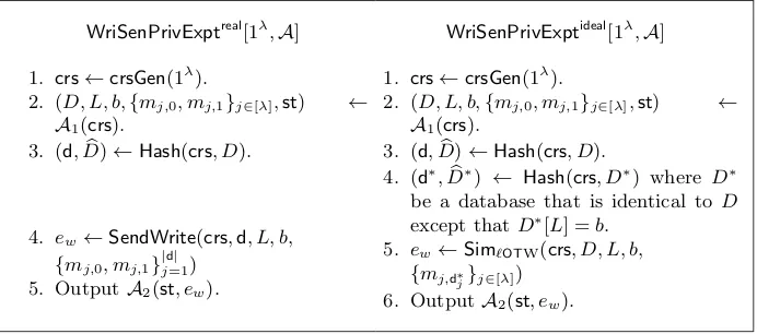
Sender Privacy for Writes: There exists a PPT simulatorSim`OTWsuch that the for any non-uniform PPT adversary A= (A1,A2)there exists a negli-gible functionnegl(·)s.t.,
Pr[WriSenPrivExpt
real
(1λ,A) = 1]−Pr[WriSenPrivExptideal(1λ,A) = 1]
≤negl(λ)
whereWriSenPrivExptreal andWriSenPrivExptideal are described in Figure 2.
WriSenPrivExptreal[1λ,A]
1. crs←crsGen(1λ).
2. (D, L, b,{mj,0, mj,1}j∈[λ],st) ←
A1(crs).
3. (d,Db)←Hash(crs, D).
4. ew←SendWrite(crs,d, L, b, {mj,0, mj,1}|j=1d| )
5. OutputA2(st, ew).
WriSenPrivExptideal[1λ,A]
1. crs←crsGen(1λ).
2. (D, L, b,{mj,0, mj,1}j∈[λ],st) ←
A1(crs).
3. (d,Db)←Hash(crs, D).
4. (d∗,Db∗) ← Hash(crs, D∗) where D∗ be a database that is identical to D except thatD∗[L] =b.
5. ew←Sim`OTW(crs, D, L, b, {mj,d∗j}j∈[λ])
6. OutputA2(st, ew).
Figure 2: Sender Privacy for Writes Security Game
Efficiency: The algorithm Hash runs in time|D|poly(log|D|, λ). The algorithms
Theorem 2 ([CDG+17]).AssumingiOfor circuits andsomewhere statistically binding hash functions, there exists a construction of updatable laconic oblivious transfer.
Remark 2. We note that the security requirements given in Definition 5 is stronger than the one in [CDG+17] as we require thecrsto be generated before the
ad-versary provides the databaseDand the locationL. However, the constructions given in [CDG+17] already satisfies this stronger definition and this was noted
in [GS18a].
A Note on Hash Updates.The construction of updatable Laconic Oblivious Transfer given in [CDG+17] uses a Merkle Hash to hash the database. Thus, to compute the hash we need the contents of the entire database to be specified. But in our construction of succinct randomized encodings, we need a methodology to compute the Merkle tree “on the fly.” More specifically, let us consider a scenario wherein we are not initially specified the entire database D∈ {0,1}M but are only given the contents of the firstnlocations. We give a methodology to compute the Merkle hash which “binds” the firstnlocations, keeps the other locations to be unspecified and runs in timepoly(n, λ,logM). A similar trick has been used in [OPWW15].
Let us assume that we are given a hash function H : {0,1}2λ → {0,1}λ. To store a database of sizeM, the Merkle tree consists ofM leaves where each leaf stores a λ bit string which either corresponds to the bit 0, or the bit 1 or a special symbol⊥ (using some canonical encoding). We construct the Merkle tree in a bottom-up fashion by labeling all the internal nodes. The label of the root node gives the hash value. We label each internal node of the Merkle tree with children given labelslab`andlabras follows:
– If bothlab` andlabrare given labels⊥, then node is given⊥as its label.
– Otherwise, the node is givenH(lab`klabr) as the label wherek denotes con-catenation.
Note that if all the locations are unspecified then the label of the root corresponds to ⊥. For each additional locationL that is specified, we just fix the auxiliary information aux to be labels of the all the nodes in the root to the leaf given by L along with their siblings. Note we only need to maintain the state of all labels which are not equal ⊥ when performing an hash update. Given this information, we can easily recompute the label of the root. This gives the required methodology to update the hash value in timepoly(n, λ,logM) wheren is the number of specified locations.
2.6 Puncturable Pseudorandom Function
Definition 6. A puncturable pseudorandom function PPRF is a tuple of PPT algorithms(KeyGenPPRF,
PRF,Punc)with the following properties:
– Efficiently Computable: For all λ and for all S ← KeyGenPPRF(1λ),
PRFS :{0,1}λ→ {0,1}λ is polynomial time computable.
– Functionality is preserved under puncturing: For all λ, for all y ∈ {0,1}λ and∀x6=y,
Pr[PRFS{y}(x) =PRFS(x)] = 1
whereS←KeyGenPPRF(1λ)andS{y} ←Punc(S, y).
– Pseudorandomness at punctured points:For allλ, for ally∈ {0,1}λ,
and for all poly sized adversariesA
|Pr[A(PRFS(y), S{y}) = 1]−Pr[A(Uλ, S{y}) = 1]| ≤negl(λ)
whereS←KeyGenPPRF(1λ),S{y} ←Punc(S, y)andU
λdenotes the uniform
distribution over{0,1}λ.
Remark 3. We can generalize the puncturing procedure to puncture at multiple points y1, . . . , ym. The security requirement now is that even given the punc-tured key S{y1, . . . , ym}, the PRF evaluations on inputs y1, . . . , ym are com-putationally indistinguishable to random. We note that in the case of multiple puncturings, the size of the punctured keyS{y1, . . . , ym} grows polynomially in
mandλ.
3
Construction of Succinct Randomized Encoding
In this section, we give a construction of succinct randomized encoding for suc-cinctly describable Turing machines. More formally, we show that:
Theorem 3. Assuming the existence of indistinguishability obfuscation and up-datable laconic oblivious transfer, there exists a construction of succinct random-ized encoding.
As shown in [BGL+15], a succinct randomized encoding with sub-exponential security gives a construction of succinctiOfor Turing machines. For complete-ness, we sketch the details of this transformation in the full version of our pa-per [GS18b]. We give the formal description of our construction of succinct ran-domized encodings in Figure 3 and give an overview below.
Overview.Let us start with an overview of the encoding scheme. The encoding procedure takes as input a description of the Turing machine M and an input
x on which the machine has to be evaluated. The procedure first reduces M
to a circuit Csc (as given in Lemma 1) that succinctly represents the circuit C
gates withN being the output gate. Each gateg∈[n+ 1, N] is described by a tuple (i, j, fg)∈[g−1]2×GTypewhere outputs of gatesiandjserves as inputs to gate g and fg is the binary function computed by gate g. Given an input
g∈[n+ 1, N], the succinct circuitCsc outputs (i, j, fg).
For our construction, we consider an alternate view of the circuitC. We view the circuitCas a sequence of step circuitsSCn+1, . . . ,SCN along with a database
D. The database is initially loaded with the inputxand each step circuit writes a single bit to the database. More precisely, for each g ∈ [n+ 1, N], the step circuit SCg implements the functionality of the gate g and writes the output of that gate to positiong in the database. Further, the step circuits access the database via an updatable laconic OT. Specifically, the step circuitSCg takes as input the digest of the database where the firstg−1 cells are filled appropriately and the rest of the positions being⊥. Using the digest, it reads the contents of the database in positions i and j (where (i, j) are the inputs to gate g) using the Send function of laconic OT. Once it has read the contents of those two locations, it applies the function fg on those two bits and writes the output to the location g using theSendWritefunction. It passes on the updated digest to the next circuit SCg+1. Thus, each of the step circuits faithfully model the
computation of the corresponding gate and the contents in location N of the database gives the output of the circuitC.
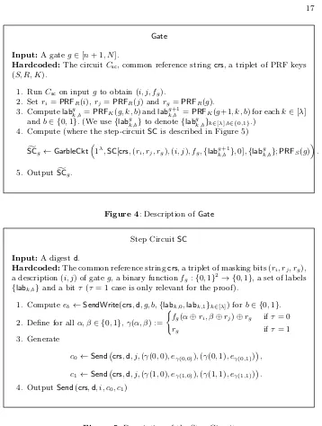
Let us now explain how the encoding procedure uses the above view of the circuit. The encoding procedure obfuscates the functionGate(formally described in Figure 4). The functionGateon inputg∈[n+ 1, N], uses the succinct circuit
Csc to get the description of gate g. Next, it constructs the step circuit SCg (formally described in Figure 5) and garbles the circuit (the randomness and the labels are derived using a puncturable pseudorandom function). The Gate
function finally outputs the garbled step circuitSCfg. The output of the encoding function is this obfuscation along with the labels corresponding to the initial digest of the database (where the input is loaded).
Given an obfuscation of the functionGate, a decoder can run this obfuscation on every gate g ∈ [n+ 1, N] to obtain the garbled step circuit SCfg. Given the labels corresponding to the initial digest, the decoder evaluates each of the garbled step circuits fromn+ 1 toN (labels corresponding to thegthstep circuit are output by the (g−1)thcircuit). At the end of the computation, the content of the database at locationN gives the output.
However, there is one technical issue. Recall that the laconic OT is not guar-anteed to hide the contents of the database. In order to hide the contents of the database, we use a one-time pad to mask each bit that is written. This one time pad is succinctly derived using a puncturable pseudorandom function.
Correctness.This argument is based on the correctness proof in [GS18a]. Let
Dg∗ be the contents of the database at the beginning ofg∗-th iteration of the forloop insRE.Dec. We first argue via an inductive argument that for each gate
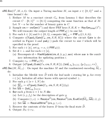
sRE.Enc(1λ, M, x, t): On input a Turing machineM, an inputx∈ {0,1}n and a time boundtdo:
1. Reduce M to a succinct circuit Csc from Lemma 1 that describes the circuit C :{0,1}n → {
0,1}computing the same function as that ofM. LetN−nbe the number of binary gates inC.
2. Samplecrs←crsGen(1λ) and three PRF keysS, R, K←KeyGenPPRF(1 λ
). We will truncate the output length ofPRFR(·) to one bit.
3. For eachk∈[λ] andb∈ {0,1}, computelab1
k,b=PRFK((1, k, b)). 4. Compute iO(pad`(Gate[Csc,crs, S, R, K])) where the circuit Gate is
de-scribed in Figure 4 andpad`(·) pads the circuit to size ` which will be specified in the proof.
5. For eachi∈[n], setyi=xi⊕PRFR(i). 6. Setd=⊥and for eachi∈[n],
(a) Recomputed=HashUpdate(crs,d,(i, yi),aux) whereauxis the auxil-iary information for updating positioni.
7. ComputerN=PRFR(N).
8. Output iO(pad`(Gate[Csc,crs, S, R, K])),{lab1k,dk}k∈[λ],{yi}i∈[n], rN
. sRE.Dec(M,Mx,tc ) : On input the machineM and the randomized encodingMx,tc
do:
1. Initialize the Merkle treeDb with the leaf nodeistoring bityi for every i∈[n]. Initialize all other leaves with special symbol⊥.
2. For eachg∈[n+ 1, N] do:
(a) SCfg:=iO(pad`(Gate[Csc,crs, S, R, K]))(g). 3. Setlab={lab1k,dk}k∈[λ].
4. foreachgfromn+ 1 toN do:
(a) Let (i, j, fg) be the description of gate g. (b) Compute (γ, e) :=ReceiveDb
(crs,ReceiveDb
(crs,EvalCkt(SCfg,lab), i), j). (c) Setlab:=ReceiveWriteDb
(crs, g, γ, e).
5. Recover the contents of the leavesDfrom the final stateDb. 6. OutputDN⊕rN.
Figure 3: Succinct Randomized Encoding
Given this, the correctness follows by setting g∗ := N and observing that the
DN+1,N is unmasked usingrN in Step 7 ofsRE.Dec.
The base case isg∗=nwhich is clearly true since in the beginningDn+1 is
set as (r[1,n]⊕x||⊥N−n). In order to prove the inductive step for a gateg∗(with
description (i, j, fg∗)), we now argue that that the γ recovered in Step 4.(b)
of sRE.Dec corresponds to fg∗(Dg∗,i⊕riDg∗,j⊕rj)⊕rg∗ which by inductive
hypothesis corresponds to output of the gateg∗ masked withrg∗. This is shown
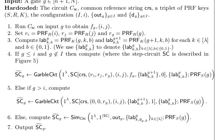
Gate
Input:A gateg∈[n+ 1, N].
Hardcoded:The circuitCsc, common reference stringcrs, a triplet of PRF keys (S, R, K).
1. RunCscon inputgto obtain (i, j, fg).
2. Setri=PRFR(i),rj=PRFR(j) andrg=PRFR(g).
3. Computelabgk,b=PRFK(g, k, b) andlabg+1k,b =PRFK(g+1, k, b) for eachk∈[λ] andb∈ {0,1}. (We use{labgk,b}to denote{labgk,b}k∈[λ],b∈{0,1}.)
4. Compute (where the step-circuitSCis described in Figure 5)
f
SCg←GarbleCkt
1λ,SC[crs,(ri, rj, rg),(i, j), fg,{labg+1k,b },0],{labgk,b};PRFS(g)
.
5. OutputSCfg.
Figure 4: Description ofGate
Step CircuitSC
Input:A digestd.
Hardcoded:The common reference stringcrs, a triplet of masking bits (ri, rj, rg), a description (i, j) of gateg, a binary functionfg:{0,1}2→ {
0,1}, a set of labels {labk,b}and a bitτ (τ = 1 case is only relevant for the proof).
1. Computeeb←SendWrite(crs,d, g, b,{labk,0,labk,1}k∈[λ]) forb∈ {0,1}.
2. Define for allα, β∈ {0,1},γ(α, β) := (
fg(α⊕ri, β⊕rj)⊕rg ifτ = 0
rg ifτ = 1
3. Generate
c0←Send crs,d, j,(γ(0,0), eγ(0,0)),(γ(0,1), eγ(0,1)) ,
c1←Send crs,d, j,(γ(1,0), eγ(1,0)),(γ(1,1), eγ(1,1)) .
4. OutputSend(crs,d, i, c0, c1)
Figure 5: Description of the Step Circuit
(γ, e) :=ReceiveDb(crs,ReceiveDb(crs,EvalCkt(fSC
g,lab), i), j) = ReceiveDb
(crs,ReceiveDb
(crs,Send(crs,d, i, c0, c1), i), j) = ReceiveDb(crs, c
Dg∗,i, j)
= ReceiveDb
crs,Sendcrs,d, j,(γ(Dg∗,i,0), eγ(D
g∗,i,0)),(γ(Dg∗,i,1), eγ(Dg∗,i,1))
, j
= γ(Dg∗,i, Dg∗,j), eγ(D
g∗,i,Dg∗,j)
= fg∗(Dg∗,i⊕riDg∗,j ⊕rj)⊕rg∗, ef
g∗Dg∗,i⊕riDg∗,j⊕rj⊕rg∗
4
Security Proof
In this section, we prove that the construction presented in the Section 3 satisfies security property given in Definition 2. In Subsection 4.1, we start by defining circuit configurations. Next, in Subsection 4.2 we show that both the real world garbling procedure and the simulated distributions are special cases of this circuit configuration. Finally, in the rest of the subsection we show that the real garbling and the simulated distributions are indistinguishable.
4.1 Circuit Configuration
Our proof of security proceeds via a hybrid argument over differentcircuit con-figurations which we describe in this section. A circuit configuration denoted by conf = (I, i) consists of a set I ⊆ [n+ 1, N] and an index i ∈ [n+ 1, N]. Intuitively, each circuit configuration defines a distribution of the randomized encodingMcx,tconf. Let us now explain the semantics of the setI and the indexi.
Recall that from our construction described in Figure 3,iO(pad`(Gate)) out-puts SCfg when given a gateg∈[n+ 1, N] as input. Intuitively, a configuration of a circuit defines a particular distribution of SCfg for each g ∈ [n+ 1, N]. In particular, for each gate g, the distribution of SCfg can be in one of the three modes:Whitemode,Graymode and theBlackmode. We say thatSCfgis said to be in White mode if for the distribution of SCfg is same as the honest garbling procedure given in Figure 4. We say thatSCfg is inGraymode if its distribution depends only on the output of the gate g when the circuitC is evaluated with inputx. We say thatSCfg is in Blackmode if its distribution is independent of the inputx. Looking ahead, initially all the step circuits will be inWhite mode and the goal will be to convert all of them to Blackin the simulation. We will achieve this in the reverse order i.e., we first change SCN to Black mode and then changeSCN−1and so on. The indexi(given as part of defining the circuit
configuration) is such that for all g > ithe distribution of the garbled step cir-cuitSCfgis inBlackmode. We can also extend the notion ofBlackmode to input gates [1, n]. So i can be any element in the set [0, N]. The subset I indicates the set of gatesgsuch that the distribution of the garbled step circuitSCfg is in
Graymode. The rest of the garbled step circuitsSCfg whereg6∈I andg≤iare generated inWhitemode. We say a configuration is valid ifI∩[i+ 1, N] =∅.
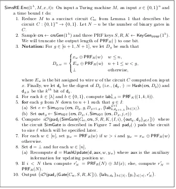
SimsRE.Enc(1λ, M, x, t): On input a Turing machineM, an inputx∈ {0,1}nand a time boundtdo:
1. Reduce M to a succinct circuit Csc from Lemma 1 that describes the circuitC:{0,1}n→ {
0,1}. LetN−nbe the number of binary gates in C.
2. Samplecrs←crsGen(1λ) and three PRF keysS, R, K←KeyGenPPRF(1 λ
). We will truncate the output length ofPRFR(·) to one bit.
3. Notation:Forg∈[n+ 1, N+ 1], we letDg be such that
Dg,w=
xw⊕PRFR(w) w≤n, Ew⊕PRFR(w) n+ 1≤w < g,
⊥ otherwise,
whereEwis the bit assigned to wirewof the circuitCcomputed on input x. Finally, we letdgbe the digest ofDg (i.e., (dg,·) :=Hash(crs, Dg)) and dg,k be thekthbit ofdg.
4. For eachk∈[λ] andb∈ {0,1}, computelab1k,b=PRFK((1, k, b)). 5. foreachgfromN down ton+ 1 such thatg∈I:
(a) Sete←Sim`OTW(crs, Dg, g, Dg+1,g,{labg+1k,dg+1,k}k∈[λ]).
(b) Setoutg ←Sim`OT(crs, Dg, i,Sim`OT(crs, Dg, j, e))
6. Compute iO(pad`(SimGate[Csc,crs, S, R, K,(I, i),{outg,dg}g∈I])) where the circuitSimGateis described in Figure 7 andpad`(·) pads the circuit to size`which will be specified later.
7. For eachw∈ [n], setyw =PRFR(w) ifw > iandyw =xw⊕PRFR(w) otherwise.
8. Setd=⊥and for eachw∈[n],
(a) Recomputed=HashUpdate(d,aux, w, yw) whereauxis the auxiliary information for updating positionw.
9. If i < N then compute r0N = PRFR(N)⊕M(x); else, compute r0N = PRFR(N).
10. Output iO(pad`(Gate[Csc, S, R, K])),{labk,dk}k∈[λ],{yi}i∈[n], r0N
.
Figure 6: Succinct Randomized Encoding in configurationconf= (I, i).
4.2 Our Hybrids
For every circuit configuration conf = (I, i), we defineHybridconf to be a distri-bution ofMcx,tas given in Figure 6. We start by observing that both real world and ideal distribution from Definition 2 can be seen as instance of Hybridconf
SimGate
Input:A gateg∈[n+ 1, N].
Hardcoded:The circuitCsc, common reference stringcrs, a triplet of PRF keys (S, R, K), the configuration (I, i),{outg}g∈I and{dg}g∈I.
1. RunCscon inputgto obtainfg,(i, j).
2. Setri=PRFR(i),rj=PRFR(j) andrg=PRFR(g).
3. Computelabgk,b=PRFK(g, k, b) andlabg+1k,b =PRFK(g+1, k, b) for eachk∈[λ] andb∈ {0,1}. (We use{labgk,b}to denote{labgk,b}k∈[λ],b∈{0,1}.)
4. If g ≤iand g6∈ I then compute (where the step-circuitSCis described in Figure 5)
f
SCg←GarbleCkt
1λ,SC[crs,(ri, rj, rg),(i, j), fg,{labg+1k,b },0],{labgk,b};PRFS(g)
.
5. Else ifg > i, compute
f
SCg←GarbleCkt
1λ,SC[crs,(0,0, rg),(i, j),{labg+1k,b },1],{labgk,b};PRFS(g)
.
6. Else, computeSCfg ←SimCkt
1λ,1|SC|,outg,{labgk,d
g,k}k∈[λ];PRFS(g)
.
7. OutputSCfg.
Figure 7: Description ofSimGate
minimizing the maximum number of gates in theGraymode in any intermediate hybrid.5
4.2.1 Rules of Indistinguishability We will now describe the two rules (we call these rule A and rule B) to move from one valid circuit configuration
conf to another valid configurationconf0such thatHybridconfis computationally indistinguishable fromHybridconf0.
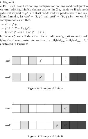
Rule A: Rule A says that for any valid configurationconfwe can indistinguish-ably change gateg∗ in White mode toGray mode if it is the first gate or if its predecessor is also in Gray mode. More formally, let conf = (I, i) and
conf0 = (I0, i0) be two valid circuit configurations andg∗ ∈ [n+ 1, N] be a gate such that:
– i=i0.
– g∗6∈I, I0 =I∪ {g∗}andg∗≤i.
– Eitherg∗=n+ 1 org∗−1∈I. 5
In Lemma 4, we will show that for two valid configurationsconf,conf0 satisfy-ing the above constraints we have thatHybridconf≈c Hybridconf0. Note that we
can also use this rule to move a gateg∗ fromGraymode toWhitemode. We refer to those invocations of the rule asinverse A rule. Rule A is illustrated in Figure 8.
Rule B: Rule B says that for any configuration for any valid configurationconf
we can indistinguishably change gate g∗ in Graymode to Blackmode if all gates subsequent tog∗is inBlackmode and the predecessor is inGraymode. More formally, let conf = (I, g∗) and conf0 = (I0, g0) be two valid circuit configurations such that:
– g∗=g0+ 1.
– g∗∈I, I0 =I\ {g∗}.
– Eitherg∗=n+ 1 org∗−1∈I.
In Lemma 5, we will show that for an valid configurationsconf,conf0 satis-fying the above constraints we have thatHybridconf≈c Hybridconf0. Rule B is
illustrated in Figure 9.
conf g∗ i
conf0 g∗ i
Figure 8: Example of Rule A
conf g∗
conf0 g0 g∗
4.2.2 Interpreting the rules of indistinguishability as a pebbling game
Sections 4.2.2 and 4.2.3 are taken verbatim from [GS18a]. Our sequence of hy-brids from the real to the ideal world follow an optimal strategy for the following pebbling game. The two rules described above correspond to the rules of our pebbling game below.
Consider the positive integer linen+ 1, n+ 2, . . . N. We are given pebbles of two colors: gray and black . A black pebble corresponds to a gate in theBlack
(i.e., input independent simulation) mode and a gray pebble corresponds to a gate in the Gray (i.e., input dependent simulation) mode. A position without any pebble corresponds to real garbling or in theWhitemode. We can place the pebbles on this positive integer line according to the following two rules:
Rule A: We can place or remove a gray pebble in positioniif and only if there is a gray pebble in positioni−1. This restriction does not apply to position
n+ 1: we can always place or remove a gray pebble at positionn+ 1.
Rule B: We can replace a gray pebble in positioniwith a black pebble as long as all the positions > i have black pebbles and there is a gray pebble in positioni−1 or ifi=n+ 1.
Optimization goal of the pebbling game. The goal is to pebble the line [n+ 1, N] such that every position has a black pebble while minimizing the number of gray pebbles that are present on the line at any point in time.
4.2.3 Optimal Pebbling Strategy To provide some intuition, we start with the na¨ıve pebbling strategy. The na¨ıve pebbling strategy involves starting from positionn+ 1 and placing a gray pebble at every position in [n+ 1, N] and then replacing them with black pebbles fromN ton+ 1. However, this strategy uses a total ofN−ngray pebbles. Using a more clever strategy, it is actually possible to do the same using only log(N−n) gray pebbles. We first recall the following lemma from [GPSZ17].
Lemma 2 ([GPSZ17]).For any integern+ 1≤p≤n+ 2k−1, it is possible to
makeO((p−n)log23)≈O((p−n)1.585) moves and get a gray pebble at position
pusingk gray pebbles.
Proof. For completeness we give the proof. This proof is taken verbatim from [GPSZ17].
First we observe to get a gray pebble placed atp, for eachi∈[n+ 1, p−1] there must have been at some point a gray pebble placed at locationi.
Next, we observe that it suffices to show we can get a gray pebble at position
p=n+ 2k−1 for everykusingO(3k) =O((p−n)log23) steps. Indeed, for more
generalp, we run the protocol for p0 =n+ 2k−1 wherek=dlog
2(p−n−1)e,
but stop the first time we get a gray pebble at position p. Since p0/p≤3, the running time is at mostO((p−n)log23).
Now for the algorithm. The sequence of steps will create a fractal pattern, and we describe the steps recursively. We assume an algorithmAk−1 usingk−1
gray pebbles that can get a gray pebble at positionn+ 2k−1−1. The steps are
– RunAk−1. There is now a gray pebble at positionn+ 2k−1−1 on the line. – Place the remaining gray pebble at positionn+ 2k−1, which is allowed since
there is a gray pebble at positionn+ 2k−1−1.
– RunAk−1in reverse, recovering all of thek−1 gray pebbles used byA. The
result is that there is a single gray pebble on the line at positionn+ 2k−1.
– Now associate the portion of the number line starting atn+ 2k−1+ 1 with a
new number line. That is, associaten+ 2k−1+aon the original number line
withn0+a(wheren0=n+2k−1) on the new number line. We now havek−1
gray pebbles, and on this new number line, all of the same rules apply. In particular, we can always add or remove a gray pebble from the first position
n0+1 =n+2k−1+1 since we have left a gray pebble atn+2k−1. Therefore, we
can runAk+1 once more on the new number line starting atn0+ 1. The end
result is a pebble at positionn0+2k−1−1 =n+2k−1+(2k−1−1) =n+2k−1. It remains to analyze the running time. The algorithm makes 3 recursive calls toAk−1, so by induction the overall running time isO(3k), as desired.
Using the above lemma, we now give an optimal strategy for our pebbling game.
Lemma 3 ([GS18a]). For any N ∈ N, there exists a strategy for pebbling
the line graph [n+ 1, N] according to rules A and B by using at most logN gray pebbles and makingpoly(N)moves.
Proof. The proof is taken verbatim from [GS18a].
The strategy is given below. For eachg fromN down ton+ 1do:
1. Use the strategy in Lemma 2 to place a gray pebble in positiong. Note that there exists a gray pebble in positiong−1 as well.
2. Replace the gray pebble in positiongwith a black pebble. This replacement is allowed since all positions> ghave black pebbles and there is a gray pebble in positiong−1.
3. Recover all the gray pebbles by reversing the moves.
The correctness of this strategy follows by inspection and the number of moves is polynomial inN.
4.3 Proof of Indistinguishability for the Rules
In this subsection, we will use the security of underlying primitives to implement the two rules.
4.3.1 Implementing Rule A
Proof. We prove this via a hybrid argument.
– Hybridconf: This is our starting hybrid and is distributed asHybrid(I,i). – Hybrid1: In this hybrid, instead of hardwiring thePPRFkeysK andSin the
circuitSimGate, we hardwire the key K that is punctured at (g∗, k, b) for every k ∈ [λ], b∈ {0,1} and S punctured at g∗. We additionally hardwire {labgk,b∗}k∈[λ],b∈{0,1} andPRFS(g∗). This blows up the size of the circuit by a factorpoly(λ). On inputg∗−1 andg∗, the circuit now uses the hardwired labels/randomness instead of computing them using thePPRF.
It can be noted that the SimGate circuits in both Hybridconf and Hybrid1
computes the exact same functionality and hence the indistinguishability betweenHybridconf andHybrid1follows from the security ofiO.
– Hybrid2: We make three changes to the SimGate.
• By conditions of Rule A, we have thatg∗−1∈I(ifg∗6=n+1). Therefore, we note that all the input labels{labgk,b∗}are not used inSimGatebut only the labels corresponding to dg∗ i.e., {labg
∗
k,dg∗,k}k∈[λ]. We just hardwire
these labels inSimGate.
• We also hardwireSCfg∗ (that is computed using randomness PRFS(g∗))
inSimGateinstead of generating it insideSimGate. • We remove the hardwired randomnessPRFS(g∗).
The computational indistinguishability betweenHybrid2fromHybrid1follows
from the security ofiOsince the function computed bySimGatein Hybrid1
andHybrid2is exactly the same.
– Hybrid3: In this hybrid, we sample the labels{labk,dg∗,k}k∈[λ] and the
ran-domness used in generatingSCfg∗ uniformly at random instead of generating
them as outputs of the puncturable PRF. The computational indistinguisha-bility betweenHybrid2and Hybrid3follows from the security of puncturable
PRF.
– Hybrid4: In this hybrid, we generateSCfg∗(that is hardwired insideSimGate)
from the simulated distribution. More formally, we generate
f
SCg∗←Simckt(1λ,1|SC|,out,{labg ∗
k,dg∗,k}k∈[λ])
whereout←SC[crs,(ri, rj, rg),(i, j, fg),{labg
∗+1
k,b },0](dg∗).
The only change in hybridHybrid3 fromHybrid2 is in the generation of the garbled circuitSCfg∗ and the security follows directly from the selective
se-curity of the garbling scheme.
– Hybrid5: In this hybrid, we change how the output value out hardwired in f
SCg∗is generated. Recall that inHybrid4this value is generated by first
com-putingc0andc1as in Figure 5 and then generatingoutasSend(crs,d, i, c0, c1).
In this hybrid, we just generatecDg∗,i and use the laconic OT simulator to
generateout. More formally,outis generated as
out←Sim`OT crs, Dg∗, i, cD g∗,i
.
– Hybrid6: In this hybrid, we change how the valuecDg∗,i is generated. Recall
from Figure 5 thatcDg∗,iis set asSend(crs,d, j,(γ(Dg∗,i,0), eγ(Dg∗,i,0)),(γ(Dg∗,i,1), eγ(Dg∗,i,1))).
We change the distribution ofcDg∗,i toSim`OT(crs, Dg∗, j, eDg∗+1,g∗), where eDg∗+1,g∗ is sampled as in Figure 5.
Computational indistinguishability between hybridsHybrid6andHybrid5 fol-lows directly from the sender privacy of the laconic OT scheme. The argu-ment is analogous to the arguargu-ment of indistinguishability betweenHybrid4
andHybrid5.
– Hybrid7: In this hybrid, we change how eDg∗+1,g∗ is generated. More
specifi-cally, we generate it using the simulatorSim`OTW. In other words,eDg∗+1,g
is generated as
Sim`OTW(crs, Dg∗, g∗, Dg∗+1,g∗,{labg ∗+1
k,dg∗+1,k}k∈[λ]).
Computational indistinguishability between hybridsHybrid6andHybrid7 fol-lows directly from the sender privacy for writes of the laconic OT scheme.
– Hybrid8−Hybrid10: In this hybrid, we reverse the changes made inHybrid1to
Hybrid3 except that we hardwire{outg∗,dg∗} in SimGateand use it to
gen-erate SCfg∗. The indistinguishability between Hybrid7 to Hybrid10 follows in
analogous manner to the indistinguishability betweenHybridconf to Hybrid3. Finally, observe that hybridHybrid10 is the same asHybridconf0.
This completes the proof of the lemma. We additionally note that the above sequence of hybrids is reversible. This implies the inverse rule A.
4.3.2 Implementing Rule B
Lemma 5 (Rule B). Let conf and conf0 be two valid circuit configurations satisfying the constraints of rule B, then assuming the security of somewhere equivocal encryption, garbling scheme for circuits and updatable laconic oblivious transfer, we have that Hybridconf≈c Hybridconf0.
Proof. We prove this via a hybrid argument starting withHybridconf0 and ending
in hybrid Hybridconf. We follow this ordering of the hybrids as this keeps the
proof very close to the proof of Lemma 4.
– Hybridconf0: This is our starting hybrid and is distributed asHybrid(I0,g0). – Hybrid1: In this hybrid, instead of hardwiring the PPRFkeysK,RandSin
the circuit SimGate, we hardwire the key K that is punctured at (g∗, k, b) for everyk∈[λ], b∈ {0,1}, R andS are punctured atg∗. We additionally hardwire{labgk,b∗}k∈[λ],b∈{0,1}, (ri, rj,g),PRFR(g∗) andPRFS(g∗). This blows up the size of the circuit by a factor poly(λ). On input g∗−1 and g∗, the circuit now uses the hardwired labels/randomness instead of computing them using the PPRF. Note that by constraints on conf and conf0, PRFR(g∗) is only needed on inputg∗. This is because all gatesg > g∗ are inBlackmode. It can be noted that the SimGate circuits in both Hybridconf and Hybrid1
– Hybrid2: We make three changes to the SimGate.
• By conditions of Rule A, we have thatg∗−1∈I(ifg∗6=n+1). Therefore,
we note that all the input labels{labgk,b∗}are not used inSimGatebut only the labels corresponding to dg∗ i.e., {labg
∗
k,dg∗,k}k∈[λ]. We just hardwire
these labels inSimGate.
• We also hardwireSCfg∗(whereSCg∗ hasrg∗hardwired andSCfg∗ is
com-puted using randomness PRFS(g∗)) inSimGate instead of generating it insideSimGate.
• We remove the hardwired randomnessPRFS(g∗) andPRFR(g∗). The computational indistinguishability betweenHybrid2fromHybrid1follows from the security ofiOsince the function computed bySimGatein Hybrid1
andHybrid2is exactly the same.
– Hybrid3: In this hybrid, we sample the labels {labk,dg∗,k}k∈[λ], PRFR(g
∗)
and the randomness used in generating SCfg∗ uniformly at random instead
of generating them as outputs of the puncturable PRF. The computational indistinguishability betweenHybrid2andHybrid3follows from the security of puncturable PRF.
– Hybrid4: In this hybrid, we generateSCfg∗(that is hardwired insideSimGate)
from the simulated distribution. More formally, we generate
f
SCg∗←Simckt(1λ,1|SC|,out,{labg ∗
k,dg∗,k}k∈[λ])
whereout←SC[crs,(0,0, rg),(i, j, fg),{lab g∗+1
k,b },1](dg∗).
The only change in hybridHybrid3 fromHybrid4 is in the generation of the
garbled circuitSCfg∗ and the security follows directly from the selective
se-curity of the garbling scheme.
– Hybrid5: In this hybrid, we set change how the output value outhardwired in SCfg∗ is generated. Recall that in hybrid Hybrid4 this value is generated
by first computing c0 and c1 as in Figure 5 and then generating out as
Send(crs,d, i, c0, c1). In this hybrid, we just generate cDg∗,i and use the
la-conic OT simulator to generateout. More formally,outis generated as
out←Sim`OT crs, Dg∗, i, cD g∗,i
.
Computational indistinguishability between hybridsHybrid4andHybrid5 fol-lows directly from the sender privacy of the laconic OT scheme.
– Hybrid6: In this hybrid, we change how the how the valuecDg∗,i is generated
in hybridHybrid5. Recall from Figure 5 thatcDg∗,i is set asSend crs,d, j, erg∗, erg∗
. We change the distribution ofcDg∗,i toSim`OT crs, Dg, j, erg∗
, whereerg∗
is sampled as in Figure 5.
Computational indistinguishability between hybridsHybrid5andHybrid6 fol-lows directly from the sender privacy of the laconic OT scheme. The argu-ment is analogous to the arguargu-ment of indistinguishability betweenHybrid4
– Hybrid7: In this hybrid, we change how erg∗ is generated. More specifically,
we generate it using the simulatorSim`OTW. In other words,erg∗ is generated
as
Sim`OTW(crs, Dg∗, g∗, rg∗,{labg ∗+1
k,dg∗+1,k}k∈[λ]).
Computational indistinguishability between hybridsHybrid6andHybrid7 fol-lows directly from the sender privacy for writes of the laconic OT scheme.
– Hybrid8: The only difference betweenHybrid7andHybrid8is howDg∗+1,g∗is
set. Namely, inHybrid7this value is set to berg∗ while inHybrid8this value
is set as rg∗⊕fg∗(Dg∗,i⊕ri, Dg∗,j⊕rj). We argue that the distributions Hybrid7andHybrid8are identical. Two cases arise:
• g∗≤N−1: In this case, note that sincerg∗ is not hardwired anywhere
else, we have that the distributionrg∗andrg∗⊕fg∗(Dg∗,i⊕riDg∗,j⊕rj)
are both uniform and identical. • g∗ = N: In this case, we have that r
g∗ = M(x)⊕r0g∗ which is again
identical to the distribution ofrg∗ inHybrid8.
– Hybrid9−Hybrid11: In this hybrid, we reverse the changes made inHybrid1to
Hybrid3 except that we hardwire{outg∗,dg∗} in SimGateand use it to
gen-erateSCfg∗.. The indistinguishability between Hybrid8 toHybrid11 follows in
analogous manner to the indistinguishability betweenHybridconf0 toHybrid3.
Observe thatHybrid11is distributed identically toHybridconf. This completes the proof of the lemma.
4.3.3 Completing the Hybrids The strategy given in Lemma 3 yields a sequence of configurationsconf0. . .confmfor an appropriate polynomialmwith
conf0= (∅, N) andconfm= (∅, n), whereHybridconfi−1 c
≈Hybridconf
i either using
rule A (i.e., Lemma 4) or using rule B (i.e., Lemma 5). We now show that
Hybridconfm is computationally indistinguishable to the ideal world distribution given byHybrid(∅,0). This is argued using the security property of puncturable PRF using the keyRand the security ofiOas follows.
– Hybrid1 : In this hybrid, we puncture the PRF key R at points {1, . . . , n} and hardwire it inSimGate. Note that inHybrid(∅,n), the functionSimGate
never uses the PRF key on inputs {1, . . . , n} and hence the functionality computed by theSimGateis exactly the same in this hybrid andHybrid(∅,n).
The computational indistinguishability follows from the security ofiO.
– Hybrid2: In this hybrid, we replaceywwith a random bitrwfor eachw∈[n]. The computational indistinguishability betweenHybrid1 andHybrid2 follows from the security of puncturable PRF.
– Hybrid3: In this hybrid, we replaceywwithPRFR(w) for everyw∈[n]. The computational indistinguishability betweenHybrid2andHybrid3follows from the security of puncturable PRF.
Finally, the padding size ` is set to be maximum over the sizes of SimGate in every intermediate hybrid in the proof of Lemma 4, Lemma 5 and in the proof of indistinguishability betweenHybrid(∅,n)andHybrid(∅,0). This is observed to be
poly(|M|,logN, λ, n). This completes the proof of security.
References
[AIK04] Benny Applebaum, Yuval Ishai, and Eyal Kushilevitz. Cryptography in NC0. In 45th Annual Symposium on Foundations of Computer Science, pages 166–175, Rome, Italy, October 17–19, 2004. IEEE Computer Society Press.
[AJ15] Prabhanjan Ananth and Abhishek Jain. Indistinguishability obfuscation from compact functional encryption. In Rosario Gennaro and Matthew J. B. Robshaw, editors,Advances in Cryptology – CRYPTO 2015, Part I, volume 9215 ofLecture Notes in Computer Science, pages 308–326, Santa Barbara, CA, USA, August 16–20, 2015. Springer, Heidelberg, Germany. [AL18] Prabhanjan Ananth and Alex Lombardi. Succinct garbling schemes from
functional encryption through a local simulation paradigm. To appear in TCC, 2018. https://eprint.iacr.org/2018/759.
[App17] Benny Applebaum. Garbled circuits as randomized encodings of functions: a primer. Cryptology ePrint Archive, Report 2017/385, 2017. http:// eprint.iacr.org/2017/385.
[BGI+12] Boaz Barak, Oded Goldreich, Russell Impagliazzo, Steven Rudich, Amit Sahai, Salil P. Vadhan, and Ke Yang. On the (im)possibility of obfuscating programs. J. ACM, 59(2):6, 2012.
[BGI14] Elette Boyle, Shafi Goldwasser, and Ioana Ivan. Functional signatures and pseudorandom functions. In Public-Key Cryptography - PKC 2014 - 17th International Conference on Practice and Theory in Public-Key Cryptography, Buenos Aires, Argentina, March 26-28, 2014. Proceedings, pages 501–519, 2014.
[BGL+15] Nir Bitansky, Sanjam Garg, Huijia Lin, Rafael Pass, and Sidharth Telang. Succinct randomized encodings and their applications. In Rocco A. Serve-dio and Ronitt Rubinfeld, editors,47th Annual ACM Symposium on The-ory of Computing, pages 439–448, Portland, OR, USA, June 14–17, 2015. ACM Press.
[BGT14] Nir Bitansky, Sanjam Garg, and Sidharth Telang. Succinct randomized encodings and their applications. Cryptology ePrint Archive, Report 2014/771, 2014. http://eprint.iacr.org/2014/771.
[BHR12] Mihir Bellare, Viet Tung Hoang, and Phillip Rogaway. Foundations of garbled circuits. In Ting Yu, George Danezis, and Virgil D. Gligor, edi-tors,ACM CCS 12: 19th Conference on Computer and Communications Security, pages 784–796, Raleigh, NC, USA, October 16–18, 2012. ACM Press.
[BLSV18] Zvika Brakerski, Alex Lombardi, Gil Segev, and Vinod Vaikuntanathan. Anonymous ibe, leakage resilience and circular security from new assump-tions. To appear in Eurocrypt, 2018. https://eprint.iacr.org/2017/ 967.