Title: Eccentricity-dependent temporal contrast tuning in human visual cortex measured with fMRI.
Authors and Affiliations: Marc M. Himmelberg1* & Alex R. Wade1,2
1 Department of Psychology, The University of York, Heslington, York, YO10 5DD, United Kingdom.
2 York NeuroImaging Centre, The Biocentre, York Science Park, Heslington, York, YO10 5NY, United Kingdom.
Corresponding Author: Marc M. Himmelberg, Department of Psychology, The University of York, York, YO10 5DD, UK (email: [email protected])
1
2
3
4
5
6
7
8
9
10
11
12
13
14
15
16
17
18
19
Abstract
Cells in the peripheral retina tend to have higher contrast sensitivity and respond at higher flicker frequencies than those closer to the fovea. Although this predicts increased behavioural temporal contrast sensitivity in the peripheral visual field, this effect is rarely observed in psychophysical experiments. It is unknown how temporal contrast sensitivity is represented across eccentricity within cortical visual field maps and whether such sensitivities reflect the response properties of retinal cells or psychophysical sensitivities. Here, we used functional magnetic resonance imaging (fMRI) to measure contrast sensitivity profiles at four temporal frequencies in five retinotopically-defined visual areas. We also measured population receptive field (pRF) parameters (polar angle, eccentricity, and size) in the same areas. Overall contrast sensitivity, independent of pRF parameters, peaked at 10Hz in all visual areas. In V1, V2, V3, and V3a, peripherally-tuned voxels had higher contrast sensitivity at a high temporal frequency (20Hz), while hV4 more closely reflected behavioural sensitivity profiles. We conclude that our data reflect a cortical representation of the increased peripheral temporal contrast sensitivity that is
21
22
23
24
25
26
27
28
29
30
31
32
33
34
35
36
37
38
39
already present in the retina and that this bias must be compensated later in the cortical visual pathway.
Keywords: visual cortex; temporal contrast sensitivity; magnocellular pathway; eccentricity; fMRI; population receptive fields
Introduction
There is a mismatch between electrophysiological retinal measurements and psychophysical measurements of temporal contrast sensitivity across the visual field. Eccentricity-dependent differences in retinal temporal sensitivity originate in the cone photoreceptors – peripheral cones respond faster and are more sensitive to flicker when compared to those in the fovea (Sinha et al., 2017). These signals are filtered through the retinal ganglion cells (RGCs), where there is an increase in the proportion of parasol to midget RGCs with increasing retinal eccentricity (Connolly & van Essen, 1984; Dacey, 1993, 1994; Dacey & Petersen, 1992; De Monasterio & Gouras, 1975). Temporal frequency sensitivity is thought to be related to the relative
41
42
43
44
45
46
47
48
49
50
51
52
53
54
55
56
57
58
parvocellular pathway, respectively (Hammett, Thompson, & Bedingham, 2000; Harris, 1980). On average, RGCs in the periphery have larger receptive fields and cells with such receptive fields have increased contrast sensitivity (Dacey & Petersen, 1992; Enroth-Cugell & Shapley, 1973). Overall then, the peripheral retina has relatively more parasol cells, those cells integrate from larger portions of the retina, and they are fed by cones with brisker response kinetics (Dacey & Petersen, 1992; Enroth-Cugell & Shapley, 1973; Sinha et al., 2017). From such physiological differences we might expect subjects to be more sensitive to low contrast flickering stimuli in the periphery of the visual field.
These predictions are not generally confirmed by psychophysical measurements of temporal contrast sensitivity across space. Previous research has found that psychophysical temporal contrast thresholds are approximately independent of visual field eccentricity (Koenderink, Bouman, Bueno, & Slappendel, 1978; Virsu, Rovamo, Laurinen, & Näsänen, 1982; Wright & Johnston, 1983). Although such thresholds (which by definition, occur at relatively low contrast) are independent of eccentricity, very low spatial frequencies might be an exception: previous papers report an increase in critical flicker frequency with increasing eccentricity (Hartmann, Lachenmayr, & Brettel, 1979; Rovamo & Raninen, 1984). How these eccentricity-dependent sensitivities to temporal contrast are represented in the visual cortex is currently unknown.
61
62
63
64
65
66
67
68
69
70
71
72
73
74
75
76
77
78
79
The early visual cortex is organised retinotopically; visual space is mapped topographically, with foveal receptive fields mapped towards the occipital pole and more peripheral receptive fields mapped in increasingly anterior areas of the cortex (Engel, Glover, & Wandell, 1997). Perhaps then, investigating sensitivity to temporal contrast across cortical space can help to explain the discrepancy between measurements of retinal and psychophysical temporal contrast sensitivity. Previous research has found centrally located sustained and peripherally located transient temporal channels in primary visual cortex, and these channels are thought to reflect responses from different classes of cells (Horiguchi, Nakadomari, Masaya, & Wandell, 2009). One might ask whether the relative weighting of response properties of peripheral retinal cells to temporal frequency and contrast is maintained in V1 and other early visual areas. One might also ask at what point in the cortical pathway is temporal contrast sensitivity filtered to reflect psychophysical sensitivity across space, rather than retinal sensitivity. One might expect such filtering to occur in higher-order visual areas that are typically specialized for complex feature identification computations that do not require temporal frequency information.
How do measurements of cortical temporal contrast sensitivity across space relate to behaviour? To answer this, we used fMRI to measure voxel contrast response functions (CRFs) at a range of temporal frequencies and plotted responses as a function of pRF eccentricity in different visual areas. Additionally, we obtained
81
82
83
84
85
86
87
88
89
90
91
92
93
94
95
96
97
98
99
psychophysical temporal contrast threshold measurements in central and near-peripheral regions of visual space. Previous research has found that the optimal contrast sensitivity of the primate visual system is approximately 8Hz, thus we predicted that we would observe a similar peak contrast sensitivity, independent of eccentricity, in our psychophysical and fMRI data (Hawken, Shapley, & Grosof, 1996; Kastner et al., 2004; Singh, Smith, & Greenlee, 2000; Venkataraman, Lewis, Unsbo, & Lundström, 2017). Next, due to retinal biases, we predicted that in early visual areas, contrast sensitivity would be greater at a high temporal frequency in pRFs representing more peripheral locations. Conversely, if cortical sensitivities are to shift to be more reflective of behaviour at some point in the cortex, it is predicted that such areas will show no difference in temporal contrast sensitivity across pRF eccentricity.
Materials and Methods
Participants
Nineteen participants (mean ± SD age, 27.89 ± 5.72; 9 males) were recruited from the University of York. All participants had normal or corrected to normal vision. Each participant completed a 1-hour psychophysics session and two 1-hour fMRI sessions. In the first fMRI session, two high-resolution structural scans and six pRF functional runs were obtained. In the second fMRI session, 10 temporal contrast
101
102
103
104
105
106
107
108
109
110
111
112
113
114
115
116
117
118
119
sensitivity (TCS) functional runs were obtained. All participants provided informed consent before participating in the study. Experiments were conducted in accordance with the Declaration of Helsinki and the study was approved by the ethics committees at the York NeuroImaging Centre and the University of York Department of Psychology.
Behavioural Psychophysics
Experimental Design
To investigate psychophysical temporal contrast sensitivity, we measured contrast detection thresholds for four temporal frequency conditions (1, 5, 10, and 20Hz) at two eccentricities (2° and 10°). 75% correct detection thresholds were obtained using a ‘2 Alternative Forced Choice’ (2AFC) method using four randomly interleaved Bayesian staircases in separate eccentricity blocks (Kontsevich & Tyler, 1999). A single block of 200 trials (50 of each temporal frequency condition) was presented at either 2° or 10° from central fixation on the temporal visual field meridian. Participants were instructed to maintain fixation on a central cross and to respond, via keyboard press, whether the stimulus grating appeared on the left or right of fixation. Participants were informed via a toned ‘beep’ if their response was correct or incorrect. These responses were recorded using Psykinematix software (KyberVision, Montreal, Canada, psykinematix.com). After each response, a
121
122
123
124
125
126
127
128
129
130
131
132
133
134
135
136
137
138
139
separate toned ‘beep’ was presented in conjunction with the fixation crossed briefly changing to ‘o’ then back to ‘x’ to signify the onset succeeding trial, which then began 500ms later. The first 10 trials were practice and not included in the analysis. The temporal frequency of the stimulus was randomized within each block. Participants completed each eccentricity condition block four times and responses were fit with Weibull functions of stimulus contrast. This resulted in four 75% contrast detection thresholds for each temporal frequency and eccentricity combination. For each condition, the average of these 4 thresholds was the final threshold.
Stimuli
Psychophysical stimuli (see Figure 1) were designed using Psykinematix software and were presented on a NEC MultiSync 200 CRT monitor running at 120Hz. Gamma correction was performed using a ‘Spyder5Pro’ (Datacolor, NJ, USA) display calibrator. Stimuli were circularly windowed sine wave gratings outlined with thin white circles to eliminate spatial uncertainty (Pelli, 1985). Grating spatial frequency was set to 1 cycle per degree (cpd) and were presented for 500ms. At 2° eccentricity, the grating had a 0.5° radius. Using M-scaling to account for cortical magnification, at 10° eccentricity our stimulus had a 1.021° radius (Rovamo & Virsu, 1979).
141
142
143
144
145
146
147
148
149
150
151
152
153
154
155
156
157
158
159
Figure 1: 2AFC stimulus at two eccentricity conditions. In A) a flickering stimulus grating appearing in the right circle at 2° eccentricity, while in B) the flickering stimulus grating appears in the right circle at 10° eccentricity. Participants must select which circle the grating appears in.
Functional neuroimaging
fMRI Stimulus Display
Stimuli were presented in the scanner using an PROpixx DLP LED projector (VPixx Technologies Inc., Saint-Bruno-de-Montarvile, QC, Canada) with a long throw lens that projected the image through the waveguide behind the scanner bore and onto an acrylic screen. The image presented had a resolution of 1920 x 1080 and a refresh rate of 120Hz. Participants viewed this screen at a viewing distance of 57cm using a mirror within the scanner. Gamma correction was performed using a customized MR-safe ‘Spyder4’ (Datacolor, NJ, USA) display calibrator.
161
162
163
164
165
166
167
168
169
170
171
172
173
174
175
fMRI Data Acquisition
Scans were completed on a GE Healthcare 3 Tesla Sigma HDx Excite scanner (GE Healthcare, Milwaukee, WI). Structural scans were obtained using an 8-channel head coil (MRI Devices Corporation, Waukesha, WI) to minimize magnetic field inhomogeneity. Functional scans were obtained with a 16-channel posterior head coil (Nova Medical, Wilmington, MA) to increase signal-to-noise in the occipital lobe.
Pre-processing of structural and functional scans
Two high-resolution, T1-weighted full-brain anatomical structural scans were acquired for each participant (TR, 7.8ms; TE, 3.0ms; TI, 450ms; voxel size, 1.3 x 1.3 x 1mm3; flip angle, 20°; matrix size, 176 x 256 x 257). To improve grey-white matter contrast, the two T1 scans were aligned and then averaged together using FSL tool FLIRT (Jenkinson, Beckmann, Behrens, Woolrich, & Smith, 2012). This averaged T1 was automatically segmented using a combination of FreeSurfer (http://surfer.nmr.mgh.harvard.edu/) and FSL, and manual corrections were made to the segmentation using ITK-SNAP (http://www.itksnap.org/pmwiki/pmwiki.php) (Teo, Sapiro, & Wandell, 1997). At the beginning of each functional session, one 16-channel coil T1-weighted structural scan with the same spatial prescription as the
177
178
179
180
181
182
183
184
185
186
187
188
189
190
191
192
193
194
functional scans was acquired to aid in the alignment of functional data to the T1-weighted anatomical structural scan.
Functional data were pre-processed and analysed using MATLAB 2016a (Mathworks, MA) and VISTA software (https://vistalab.stanford.edu/software/) (Vista Lab, Stanford University). Between and within scans motion correction was performed to compensate for any motion artefacts that occurred during the scan session. Any scans with >3mm movement were removed from the analysis. This resulted in the removal of one pRF run for two participants and one temporal contrast sensitivity scan for three participants. Functional runs were averaged across all scans. Next, we used mrVista tool rxAlign to co-register the 16-chanel coil T1-weighted structural scan to the 8-channel coil T1-T1-weighted full-brain anatomical scan. First, we applied a manual alignment by using landmark points to bring the two volumes into approximate register. Next, we used a robust EM-based registration algorithm as described by Nestares & Heeger (2000) to fine tune the alignment. The final alignment was checked by eye to ensure that the automatic registration procedure optimised the fit. This alignment was used as a reference to align our functional data to our full-brain anatomical scan. These functional data were then interpolated to the anatomical segmentation.
196
197
198
199
200
201
202
203
204
205
206
207
208
209
210
211
212
213
Population Receptive Field Mapping Scans
pRF scan sessions consisted of six 6.5-minute pRF stimulus presentation runs collected using a standard EPI sequence (TR, 3000ms; TE, 30ms; voxel size, 2 x 2 x 2.5 mm3, flip angle 20°; matrix size, 96 x 96 x 39). Here, a drifting pRF bar stimulus was used to obtain retinotopic maps and estimates of pRF parameters (Dumoulin & Wandell, 2008). A single bar (width 0.5°) was swept in one of eight directions within a circular aperture (10° radius) with each sweep lasting 48 seconds. Using the conversion of visual angle to retinal eccentricity, 10° radius corresponds to mapping 2.83mm radius retinal space (Drasdo & Fowler, 1974). To stimulate a broad population of neurons, the pRF carrier consisted of pink noise at 5% contrast, where the noise pattern changed at 2Hz (see Figure 2). A 12 second (4TR) dummy run was included at the beginning of each functional run to allow for the scanner magnetization to reach a steady state. To maintain fixation throughout the scan, participants completed an attentional task where they responded, via button press, when the orientation of the fixation cross changed. This task was set up so that on average, every 2 seconds there was a 30% chance of a change in the orientation of the fixation cross.
215
216
217
218
219
220
221
222
223
224
225
226
227
228
229
230
231
232
233
Figure 2: Example of the stimulus used to obtain pRF parameter estimates. The carrier is filled with pink noise that updates at 2Hz as it drifts across the screen in 8 directions.
Using mrVista, pRF positions (i.e. eccentricity and polar angle parameters) and sizes were estimated for each voxel using the standard pRF model (Dumoulin & Wandell, 2008). In Figure 3 we present exemplar eccentricity, polar angle, and pRF size maps from one participant. Following the nomenclature of Wandell et al. (2007) we delineated five bilateral regions of interest (ROIs); V1, V2, V3, V3a, and hV4, by hand on cortical flat maps based on polar angle reversals for each participant (see Figure 3B).
235
236
237
238
239
240
241
242
243
244
245
246
Figure 3: Exemplar left hemisphere retinotopic maps with ROI border overlays presented on flattened cortical representations for one subject. In A) we present eccentricity maps in which pRF eccentricity increases with distance from the fovea. In B) we present polar angle maps, with border overlays based on polar angle reversals. In C) we present pRF size maps, that show an increase in pRF size within and between ROIs.
Temporal Contrast Sensitivity (TCS) Functional Scans
Stimulus
To investigate voxel temporal contrast sensitivity, we presented participants with a vertically oriented contrast reversing sine grating within a circular aperture (10° radius). The stimulus was generated and presented using MATLAB 2016a and Psychtoolbox v.3.0.13 (Brainard, 1997). We modulated both the contrast and temporal frequency of the grating. Within each functional run the sine wave grating was presented at 20 condition combinations of Michelson contrast (1, 4, 8, 16, and 64%) and temporal frequency flicker (1, 5, 10, and 20Hz) (Michelson, 1927). The
248
249
250
251
252
253
254
255
256
257
258
259
260
261
262
263
spatial frequency of the grating was held at 1 cpd. Each stimulus condition was presented once per run and lasted 3 seconds. A baseline condition of mean luminance was presented for 3 seconds during each run. Here, a single contrast reversal was defined as one complete on-off cycle off the stimulus. A visual representation of the experimental design is illustrated in Figure 4.
Figure 4: Visual representation of temporal contrast stimulus conditions. The sine grating can be presented at 20 temporal contrast conditions.
Data acquisition and analysis
TCS functional scan sessions consisted of ten 3.5-minute stimulus presentation runs collected using an almost identical EPI sequence to that used for the pRF mapping (TR, 3000ms; TE, 30ms; voxel size, 2 x 2 x 2.5 mm3, flip angle 20°;
265
266
267
268
269
270
271
272
273
274
275
276
277
matrix size, 96 x 96 x 39). The stimulus was presented using an event related design in which condition ordering was randomized within each run. A randomized interstimulus interval separated each condition and was jittered to last on average 6 seconds. Again, a 12 second (4TR) dummy run was included at the beginning of each functional run to allow for the scanner magnetization to reach a steady state. Participants completed the same attentional task as the pRF runs throughout the experiment.
TCS data were analysed using MATLAB 2016a and VISTA software. A general linear model (GLM) was implemented to test the contribution of stimulus condition to the BOLD time course (Friston et al., 1998). We used the default two-gamma Boynton HRF from SPM5 and fit the model to an averaged time course of BOLD signal changed for each stimulus condition by minimizing the sum of squared errors (RSS) between the predicted time series and the measured BOLD response. This resulted in 20 Beta weight estimates for each voxel, reflecting sensitivity to each stimulus condition.
Statistical Analysis
Plotting Beta Weights as a Function of Eccentricity and pRF size
Only pRF and TCS voxels with ≥10% variance explained were retained for further analysis. The pooled total voxel count for each ROI and the total voxels
279
280
281
282
283
284
285
286
287
288
289
290
291
292
293
294
295
296
297
removed for falling below 10% variance explained are presented in Table 1. For each voxel within each participant’s ROI, a pRF eccentricity value and a pRF size value was extracted from the pRF data. The same ROIs were then overlaid on each corresponding participants TCS data and 20 beta weights (1 beta weight per stimulus condition) were extracted for each voxel. Thus, each voxel was allocated 22 values: a pRF eccentricity value, a pRF size value, and 20 beta weights reflecting voxel sensitivity to each TCS stimulus condition. Polar angle values were not included in the analysis.
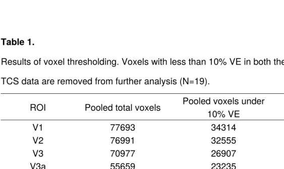
Table 1.
Results of voxel thresholding. Voxels with less than 10% VE in both the pRF and the TCS data are removed from further analysis (N=19).
ROI Pooled total voxels Pooled voxels under 10% VE
Proportion removed
V1 77693 34314 44.16%
V2 76991 32555 42.28%
V3 70977 26907 37.81%
V3a 55659 23235 41.75%
hV4 25388 25388 49.59%
For each participant, beta weights were plotted as a function of pRF eccentricity; foveal, parafoveal, or peripheral. For each ROI, foveal pRFs were defined as being between 0.2° - 3.0° eccentricity, parafoveal pRFs were defined as being between 3.0° - 6.0° eccentricity, and peripheral pRFs were defined as being
299
300
301
302
303
304
305
306
307
308
309
310
311
312
313
314
between 6.0° - 10.0° eccentricity. Visualisation of how these data are partitioned and their correspondence to visual space is illustrated in Figure 5.
Figure 5: Voxels are binned into 3 gradients of eccentricity – foveal (red), parafoveal (green), and peripheral (blue). In A) we present an eccentricity map on a right hemisphere mesh of the visual cortex with overlaid hand drawn ROIs, noting the location of V1. B) shows how these voxel bins would be represented on a schematic model of right hemisphere V1. In C) we present how the voxel bins in B) would be spatially tuned (ignoring polar angle) across the contralateral visual field.
pRF size and eccentricity are highly related measures: average pRF sizes increase with eccentricity (Dumoulin & Wandell, 2008). For completeness, we additionally analysed our data as a function of pRF size to complement the eccentricity-based analysis. Each participant’s beta weights were plotted as a function of pRF size; small or large. Receptive field sizes progressively increase as one moves up the visual hierarchy and what constitutes a ‘small’ or ‘large’ pRF will differ depending on ROI (Wandell, Dumoulin, & Brewer, 2007). To account for this,
316
317
318
319
320
321
322
323
324
325
326
327
328
329
330
331
332
within each ROI, ‘small pRFs’ were defined as having a size value between 0.25° (as a hard minimum) and the median pRF size, whilst ‘large pRFs’ were defined as a size value between the median and the maximum pRF size. These normalized pRF sizes are presented in Appendix Table A.1 and the pRF size analysis is presented in the Supplementary Materials.
Contrast response functions
For each participant’s ROIs, hyperbolic ratio functions were fitted at each of the four temporal frequencies for each eccentricity partition of data. We modelled contrast response using the following equation:
R(C)=R0+Rmax c n
c50n +cn
Where C is stimulus contrast, R0 is the baseline response, Rmax is the maximum
response rate, c50 is the semi saturation contrast, and the exponent, n, is the rate at which changes occur and was held at 2 (Albrecht & Hamilton, 1982; Boynton, Demb, Glover, & Heeger, 1999). This resulted in four contrast response functions (CRFs) per ROI at each eccentricity for each participant (i.e. each participant had four CRFs within V1 foveal, four CRFs within V1 parafoveal, and four CRFs within V1
334
335
336
337
338
339
340
341
342
343
344
345
346
347
348
349
350
351
From each CRF we extracted C50, the contrast semisaturation point. This is the amount of contrast required to elicit half the maximum response of the CRF. A decrease in C50 results in a leftward shift in the CRF, indicating that less contrast is required to hit this 50% response, thus, is representative of an increase in contrast sensitivity (Albrecht & Hamilton, 1982). Illustration of these shifts in C50 are presented in Figure 6.
Figure 6: C50 plotted on two contrast response functions. C50 decreases when the CRF is shifted left, thus less contrast is needed to hit 50% of the full response, reflecting an increase contrast sensitivity.
Analysis - Repeated Measures ANOVAs
For our psychophysical experiment, we carried out a 4 (temporal frequency) x 2 (eccentricity) repeated measures ANOVA with 75% contrast detection thresholds
354
355
356
357
358
359
360
361
362
363
364
365
366
367
as the dependent variable and looked at simple effects to compare between conditions. For our fMRI experiment we ran a 5 (ROI) x 4 (temporal frequency) x 3 (pRF eccentricity) repeated measures ANOVA with C50 as the dependent variable and looked at simple effects analyses to answer our targeted predictions.
Polynomial fits and bootstrapping
To find the temporal frequency at which contrast sensitivity peaks at each eccentricity and within each ROI (or for psychophysics, each visual field location) we used MATLAB function ‘bootstrp’ to bootstrap 2000 second order polynomial fits (generated using MATLAB function ‘polyfit’) to the means of random permutations of our contrast detection thresholds (psychophysics) and C50 data (fMRI). These data were permutated using random sampling (19 draws) with replacement. We then found the mean of the zero points of the first derivatives of each of the 2000 second order polynomial fits. This point reflects the average level of temporal frequency at which contrast sensitivity peaks.
Results
Our psychophysical data were broadly consistent with those from previous studies indicating little difference in temporal frequency tuning between fovea and
369
370
371
372
373
374
375
376
377
378
379
380
381
382
383
384
385
386
function with a minimum contrast threshold (peak sensitivity) around 8Hz. In our imaging data, we found profound changes in C50 as a function of both temporal frequency and pRF eccentricity. First, we found all visual areas studied had an overall (i.e. ignoring any effects of eccentricity) peak in contrast sensitivity at 10Hz. Next, in early visual areas we found that pRFs representing the peripheral visual field had increased contrast sensitivity at a high temporal frequency (20Hz) when compared to pRFs representing the fovea – consistent with effects predicted from retinal physiology. This difference disappeared in area hV4, where no consistent eccentricity-dependent difference in contrast sensitivity at any temporal frequency could be measured. We fed our 20Hz C50 measurements from all ROIs into a linear model and found that hV4 had the highest contribution to a fit of psychophysical contrast sensitivity. Overall, we find that contrast sensitivity in the periphery of V1, V2, V3, and V3a is increased at a high temporal frequency, but this sensitivity is lost in hV4 as cortical tuning becomes more similar that of the psychophysical observer. Here we present a summary of our results for our psychophysical and fMRI data. Supporting pRF size results are available in Supplementary Materials.
Psychophysical Results: Contrast sensitivity
A 2 x 4 repeated measures ANOVA was performed to assess whether there was a difference in psychophysical contrast detection thresholds between
389
390
391
392
393
394
395
396
397
398
399
400
401
402
403
404
405
406
407
eccentricity and temporal frequency. Mauchly’s test of Sphericity was violated for both the main effect of temporal frequency (χ2(5) = 42.321, p < .001) and the temporal frequency * eccentricity interaction effect (χ2(5) = 11.619, p = .041). Thus, a Greenhouse-Geisser correction was applied to the results of these effects.
The analysis found a significant main effect of temporal frequency (p < .001) and a significant eccentricity * temporal frequency interaction effect (p < .001). F-values and p-values are presented in Appendix Table A.2. As illustrated in Figure 7A, contrast detection thresholds were higher at 1Hz when presented at 2°
eccentricity (p < .000). Conversely, at 20Hz, contrast detection thresholds were higher at 10° eccentricity (p < .000). Thresholds significantly differed as a function of temporal frequency across both eccentricities, except for comparing between 5Hz and 10Hz. All p-values are presented in Appendix Tables A.3 and A.4.
Figure 7: Psychophysical contrast detection thresholds plotted as a function of
409
410
411
412
413
414
415
416
417
418
419
420
421
422
thresholds plotted at four measured temporal frequencies at 2° and 10°. In B) we present bootstrapped fits to contrast detection thresholds plotted as a function of temporal frequency at 2° and 10°. Overall, there is little difference in sensitivity at each temporal frequency between fovea and near periphery.
Psychophysical temporal frequency optima
To find the temporal frequency at which contrast sensitivity peaks, we looked at the mean zero point of the first derivatives of bootstrapped polynomial fits to our psychological threshold data. At 2° eccentricity contrast sensitivity peaked at 9Hz, while at 10° eccentricity contrast sensitivity peaked at 6.6Hz. Bootstrapped fits are presented in Figure 7B and mean zero points are presented in Appendix Table B.1.
fMRI Results
A 5 x 4 x 3 repeated measures ANOVA was performed to assess whether there was a difference in contrast sensitivity between ROIs, temporal frequency, and eccentricity. Mauchly’s test of Sphericity was violated for the main effect of ROI (χ2(5) = 22.062, p = .009) and the interaction effects for ROI * eccentricity (χ2(35) = 52.540, p =.036), ROI * temporal frequency (χ2(77) = 121.003, p = .003), and eccentricity * temporal frequency (χ2(20) = 42.136, p = .003). Thus, a Greenhouse-Geisser correction was applied to the results of these effects. The analysis found significant main effects for eccentricity (p = .004) and temporal frequency (p = .007).
425
426
427
428
429
430
431
432
433
434
435
436
437
438
439
440
441
442
443
444
F-values, p-values, and effect sizes for main and interaction effects are presented in Appendix Table A.5.
Contrast sensitivity peaks around 10Hz in all ROIs
First, we used a simple effects analysis to explore differences in contrast sensitivity between the four temporal frequencies, collapsed across pRF eccentricity, within each individual ROI. Sidak corrections were applied to all possible comparisons. As presented in Figure 8, V1, V2, V3, and V3a had significantly reduced C50 at 10Hz when compared to 1Hz and 20Hz (p < .05), reflecting increased contrast sensitivity at this temporal frequency. In hV4, C50 was significantly reduced 10Hz when compared to 20Hz (p = .004). P-values for these simple effects are presented in Appendix Table A.6.
446
447
448
449
450
451
452
453
454
455
456
457
Figure 8: Mean C50 values plotted as a function of temporal frequency for each ROI. C50 is consistently reduced at 10Hz in all ROIs, indicating contrast sensitivity peaks at 10Hz in all visual field maps tested.
fMRI temporal frequency optima
As we did with our psychophysical data, we looked at the mean zero point of the first derivatives of bootstrapped polynomial fits to our C50 values to find, for each ROI and eccentricity, the temporal frequency at which contrast sensitivity peaks. These zero points are presented in Appendix Table B.2 and examples of
bootstrapped fits are illustrated in Figure 9. In V1 and V2, the optimal temporal frequency gradually increased with eccentricity. However, in V3 and V3a the optimal temporal frequency increased from foveal to parafoveal. In hV4 the optimal temporal
459
460
461
462
463
464
465
466
467
468
469
470
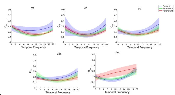
frequency is essentially identical between the foveal and parafovea. Fits to the data in the periphery of hV4 (see hV4 of Figure 9) were almost linear and no peak could be computed reliably. We attribute this to variability within the hV4 C50 estimates that were derived from the bootstrapping procedure. Thus, the peripheral hV4 fits
presented here appear to differ when compared to the corresponding mean hV4 C50 values as presented in Figure 10.
Figure 9: Examples of bootstrapped polynomial fits to C50 values plotted as a function of temporal frequency for each eccentricity in all ROIs. The solid line is a second-order bootstrapped polynomial fit to the data and the shaded outline is the standard deviation of 2000 permutations.
472
473
474
475
476
477
478
479
480
481
482
483
Figure 10: Mean C50 values plotted as a function pRF eccentricity at each temporal frequency, for each ROI. In V1-V3a, C50 is significantly reduced at 20Hz in peripheral pRFs, reflecting increased contrast sensitivity at 20Hz in the cortical periphery. This effect disappears in hV4, where C50 is flat across eccentricity at each temporal frequency.
Peripherally tuned pRFs have increased contrast sensitivity at 20Hz in V1, V2, V3,
and V3a
A simple effects analysis was undertaken to explore differences in contrast sensitivity within each ROI at each temporal frequency, comparing between foveal, parafoveal, and peripherally tuned pRFs. Sidak corrections were applied to all possible comparisons. Mean C50 values at all temporal frequencies and at 20Hz alone are presented in Figure 10. We found eccentricity-dependent differences in contrast sensitivity at 20Hz. Namely, we found that in V1, V2, V3, and V3a, C50 at
485
486
487
488
489
490
491
492
493
494
495
496
497
498
20Hz was consistently decreased in peripherally tuned pRFs when compared to foveally tuned pRFs (p < .05), reflecting increased contrast sensitivity at a high temporal frequency in the cortical periphery. There was no difference in contrast sensitivity as a function of eccentricity at 1, 5, or 10Hz, in any ROI. In Figure 11 we present a surface-based average (N=19) contrast sensitivity map at 20Hz, projected onto an inflated cortical mesh. Similar to previous psychophysical sensitivities, contrast sensitivity in hV4 was invariant across eccentricity at all temporal frequencies tested, including 20Hz. All p-values are presented in Appendix Table A.7.
Figure 11. Mean contrast sensitivity maps at 20Hz projected onto a cortical mesh (N=19). Early visual field maps V1-V3a show decreasing C50 (indicating increasing
500
501
502
503
504
505
506
507
508
509
510
511
contrast sensitivity) with increasing eccentricity, whilst contrast sensitivity in hV4 is invariant (and relatively low) across space.
Comparing psychophysical and fMRI contrast sensitivities
Unlike earlier visual areas, we found that contrast sensitivity at 20Hz in hV4 was relatively invariant across eccentricity. This finding is more similar to
psychophysical sensitivities from our own and other studies that report little difference in behavioural temporal contrast sensitivity across visual space (Koenderink et al., 1978; Virsu et al., 1982; Wright & Johnston, 1983). Next, we aimed to examine the relationship between psychophysical performance and fMRI signals driven by 20Hz stimuli. Here, we bootstrapped 1000 estimates of 20Hz fMRI C50 measurements from the fovea and periphery of each ROI, and fed this data into a linear model to assess how each ROI contributed to a fit of psychophysical contrast sensitivity at 20Hz. As illustrated in Figure 12, we found that C50 values from hV4 contributed proportionally more to our psychophysical measurements when
compared to early visual areas, indicating that fMRI responses from this area best predict our psychophysics. Bootstrapped beta weight statistics are available in Appendix Table B.3.
513
514
515
516
517
518
519
520
521
522
523
524
525
526
527
528
529
530
Figure 12. Median bootstrapped beta weights after predicting a fit of psychophysical contrast sensitivity using 20Hz C50 measurements from each ROI. hV4 has the highest beta weight, indicating that this region is the best predictor of psychophysical contrast sensitivity at 20Hz.
Discussion
We have measured differences in psychophysical and cortical contrast sensitivity that occur as a function of temporal frequency and visual field eccentricity. Overall, our findings indicate that both psychophysical and cortical contrast sensitivity follow a ‘U’ shape function and is maximal between 8-12Hz across visual space. Further, in early visual areas there is a relative increase in contrast sensitivity at 20Hz in peripherally tuned voxels. We discuss these findings in light of the physiological bias towards faster visual processing and increased contrast sensitivity
532
533
534
535
536
537
538
539
540
541
542
543
in the peripheral retina. As we moved up the visual pathway to hV4 we observed an equalisation of temporal contrast sensitivity across eccentricity that was closer to psychophysical measurements, suggesting that the bias in retinal temporal contrast sensitivity disappears in this cortical area.
Peak psychophysical and fMRI contrast sensitivity
Previous research has typically measured the primate visual system’s sensitivity to temporal frequency at a single level of contrast. These studies invariably identify a bandpass peak in temporal sensitivity occurring at approximately 8Hz (Hawken et al., 1996; Kastner et al., 2004; Kwong et al., 1992; Robson, 1966; Singh et al., 2000; Venkataraman et al., 2017). Our approach was similar to these studies, except that we fit a CRF to a range of contrasts presented at different temporal frequencies, then defined our measurement of contrast sensitivity as 50% of the full CRF response (C50). Our data showed a similar bandpass pattern. Peak psychophysical contrast sensitivity occurred at 9Hz and 6.6Hz at 2° and 10° eccentricity, respectively. Similarly, in our fMRI data we found contrast sensitivity generally peaked around 8Hz, with the critical frequency of this peak increasing between foveal and peripheral voxels. In this respect, the overall ‘U’ shape of our behavioural and cortical contrast sensitivity functions appears to be matched from a relatively early stage in the visual hierarchy.
545
546
547
548
549
550
551
552
553
554
555
556
557
558
559
560
561
562
563
Perhaps surprisingly, previous research has found little change in psychophysical temporal contrast sensitivity as a function of eccentricity (Koenderink et al., 1978; Rovamo & Raninen, 1984; Virsu et al., 1982). Although our own psychophysical data showed a slight decrease in temporal contrast sensitivity from the fovea to the near periphery, these differences were relatively small and may reflect difficulties in compensating precisely for cortical magnification effects in our own psychophysics or stimulus sizing (Granit & Harper, 1930; Hassan, Thompson, & Hammett, 2016).
Peripherally tuned pRFs have increased contrast sensitivity at 20Hz
Physiological biases in the response properties of retinal cells lead to increased temporal contrast sensitivity in more peripheral regions of the retina. Peripheral cones respond faster than foveal cones resulting in greater peripheral sensitivity to rapidly changing input (Sinha et al., 2017). There is also an eccentricity-dependent increase in the ratio of parasol to midget RGCs, and parasol cells are relatively more sensitive to high temporal frequencies and have increased contrast gain (Connolly & van Essen, 1984; Dacey, 1993, 1994; Dacey & Petersen, 1992; De Monasterio & Gouras, 1975; Schein & de Monasterio, 1987). At 10° eccentricity, measurements of temporal contrast sensitivity are thought to reflect more isolated functions of parasol RGCs (Croner & Kaplan, 1995; Gouras, 1968; Kaplan, Lee, &
565
566
567
568
569
570
571
572
573
574
575
576
577
578
579
580
581
582
583
Shapley, 1990; Kaplan & Shapley, 1986). Signals passed from RGCs pass through the LGN, where the density of afferent parasol and midget RGCs is maintained, before being sent to primary visual cortex (Connolly & van Essen, 1984; Schein & de Monasterio, 1987). Our data show that a sensitivity bias similar to that found in the retina is present in early visual cortex, with relatively increased contrast sensitivity at 20Hz in peripherally tuned voxels.
It is well known that neuronal spatial frequency sensitivity tends to be inversely related to temporal frequency sensitivity, thus, channels sensitive to low spatial frequencies are often sensitive to higher temporal frequencies (and vice versa). In addition, the sensitivity of these channels changes as a function of eccentricity (D’Souza, Auer, Frahm, Strasburger, & Lee, 2016; Henriksson, Nurminen, Hyvarinen, & Vanni, 2008; Kulikowski & Tolhurst, 1973; Shoham, Hübener, Schulze, Grinvald, & Bonhoeffer, 1997; Sun et al., 2007). Here, we report measurements made at a single spatial frequency (1 cpd). This frequency was chosen because it is well below the spatial resolution limit at the highest eccentricities measured, yet generates robust responses in the fovea (D’Souza et al., 2016; Henriksson et al., 2008; Welbourne, Morland, & Wade, 2018). It is possible that our results would change if a different spatial frequency was used: altering the base spatial frequency might, for example, alter the balance of parvo- to magnocellular cells contributing to the stimulus at each eccentricity, which would, in
585
586
587
588
589
590
591
592
593
594
595
596
597
598
599
600
601
602
603
turn, alter the average temporal response properties (Levitt, Schumer, Sherman, Spear, & Movshon, 2001).
hV4 is similar to the psychophysical observer
Unlike earlier visual areas, we found that temporal contrast sensitivity does not differ significantly as a function of eccentricity in hV4. Specifically, there appears to be little peripheral bias towards high temporal contrast. Instead, temporal contrast sensitivity in hV4 is more reflective of the behavioural observer. After bootstrapping a linear model to assess the contribution of our 20Hz C50 data to a fit of psychophysical measurements, we found that hV4 had a greater contribution to psychophysical sensitivities when compared to all other visual areas. It may be that higher order areas become increasingly invariant to eccentricity-dependent differences in low-level features, including contrast and temporal frequency, and instead represent more complex stimulus aspects relating to shape, identity, and colour (Avidan et al., 2002; Felleman & Van Essen, 1991; Milner & Goodale, 1995; Perry & Fallah, 2014). For example, hV4 has previously been found to have a much coarser representation of spatial frequency and an increased tolerance to temporal dynamics when compared to earlier visual areas, suggesting these areas are less concerned with these early visual properties (Henriksson et al., 2008; Zhou, Benson, Kay, & Winawer, 2017). In a similar vein, ventral regions local to hV4 that are concerned
605
606
607
608
609
610
611
612
613
614
615
616
617
618
619
620
621
622
623
with global form and object representations such as FFA, PPA, VO, and LOC, have at times found to be invariant to lower level visual features, and fMRI responses within such regions can become impaired when stimuli are presented at high temporal frequencies (D’Souza, Auer, Strasburger, Frahm, & Lee, 2011; Grill-Spector et al., 1999; Jiang, Zhou, & He, 2007; Kanwisher, 2010; Liu & Wandell, 2005; Mckeeff, Remus, & Tong, 2007; Vernon, Gouws, Lawrence, Wade, & Morland, 2016). Although this bias in retinal temporal contrast sensitivity is phased out by hV4, our data found that this area also responds optimally around 10Hz temporal frequency – perhaps inheriting this sensitivity bias from earlier regions.
Conclusion
Our experiments have found that in general, psychophysical and fMRI measurements of contrast sensitivity are relatively consistent and both peak around 8Hz. Voxels in early visual areas representing more peripheral regions of visual space show relatively increased contrast sensitivity to high temporal frequency when compared to those in the cortical representation of the fovea. This bias in peripheral cortical contrast sensitivity disappears by hV4, suggesting a relative independence of temporal contrast sensitivity across space in this area. This independence is broadly consistent with behavioural measurements and suggests that neurons in area hV4
625
626
627
628
629
630
631
632
633
634
635
636
637
638
639
640
641
642
(and possibly other ventral regions) are relatively invariant to the eccentricity-dependent biases that are present in the early visual stream.
Acknowledgements: M.M.H was supported by the European Union’s Horizon 2020 research and innovation programme under the Marie Skłodowska-Curie grant
agreement No 641805. A.R.W was supported by UK Biotechnology and Biological Science Research Council (BBSRC) grant number BB/M002543/1. We thank the anonymous reviewers for their constructive suggestions.
Author Contributions: M.M.H and A.R.W conceived and designed the experiments, M.M.H performed the experiments, M.M.H and A.R.W analysed the data, M.M.H wrote the paper, and M.M.H and A.R.W revised the paper.
Declaration of interest: The authors declare no competing financial interests.
References
Albrecht, D. G., & Hamilton, D. B. (1982). Striate cortex of monkey and cat: contrast response function. Journal of Neurophysiology, 48(1), 217–237.
https://doi.org/0022-3077/82/0000-0000$01.25
644
645
646
647
648
649
650
651
652
653
654
655
656
657
658
659
660
661
Smirnakis, S. M. (2002). Contrast Sensitivity in Human Visual Areas and Its Relationship to Object Recognition. Journal of Neurophysiology, 87(6), 3102– 3116. https://doi.org/10.1152/jn.2002.87.6.3102
Boynton, G. M., Demb, J. B., Glover, G. H., & Heeger, D. J. (1999). Neuronal basis of contrast discrimination. Vision Research, 39(2), 257–269.
https://doi.org/10.1016/S0042-6989(98)00113-8
Brainard, D. H. (1997). The Psychophysics Toolbox. Spatial Vision, 10(4), 433–436. https://doi.org/10.1163/156856897X00357
Connolly, M., & van Essen, D. (1984). The representation of the visualfield in parvocellular and magnocellular layers in the lateral geniculate nucleus in the macque monkey. The Journal of Comparative Neurology, 226(4), 544–564. https://doi.org/10.1002/cne.902260408
Croner, L. J., & Kaplan, E. (1995). Receptive fields of P and M ganglion cells across the primate retina. Vision Research, 35(1), 7–24. https://doi.org/10.1016/0042-6989(94)E0066-T
D’Souza, D., Auer, T., Frahm, J., Strasburger, H., & Lee, B. B. (2016). Dependence of chromatic responses in V1 on visual field eccentricity and spatial frequency: an fMRI study. Journal of the Optical Society of America. A, 33(3), 53–64. https://doi.org/10.1364/JOSAA.33.000A53
D’Souza, D., Auer, T., Strasburger, H., Frahm, J., & Lee, B. B. (2011). Temporal
664
665
666
667
668
669
670
671
672
673
674
675
676
677
678
679
680
681
682
frequency and chromatic processing in humans : An fMRI study of the cortical visual areas. Journal of Vision, 11(2011), 1–17. https://doi.org/10.1167/11.8.8 Dacey, D. M. (1993). The mosaic of midget ganglion cells in the human retina.
Journal of Neuroscience, 13(12), 5334–55.
https://doi.org/10.1523/JNEUROSCI.13-12-05334.1993
Dacey, D. M. (1994). Physiology, morphology and spatial densities of identified ganglion cell types in primate retina. In Higher-order processing in the visual system (pp. 12–34). London: Ciba Foundation.
Dacey, D. M., & Petersen, M. R. (1992). Dendritic field size and morphology of midget and parasol ganglion cells of the human retina. Proceedings of the National Academy of Sciences of the United States of America, 89(20), 9666– 9670. https://doi.org/10.1073/pnas.89.20.9666
De Monasterio, F. M., & Gouras, P. (1975). Functional properties of ganglion cells of the rhesus monkey retina. Journal of Physiology, 25(1), 167–195. https://doi.org/ 10.1113/jphysiol.1975.sp011086
Drasdo, N., & Fowler, C. W. (1974). Non-linear projection of the retinal image in a wide-angle schematic eye. British Journal of Ophthalmology, 58(8), 709–714. https://doi.org/10.1136/bjo.58.8.709
Dumoulin, S. O., & Wandell, B. A. (2008). Population receptive field estimates in human visual cortex. Neuroimage, 39(2), 647–660.
684
685
686
687
688
689
690
691
692
693
694
695
696
697
698
699
700
701
702
https://doi.org/10.1016/j.neuroimage.2007.09.034.
Engel, S. A., Glover, G. G., & Wandell, B. A. (1997). Retintopic organization in human visual cortex and the spatial precision of functional MRI. Cereb Cortex, 7(2), 181–192. https://doi.org/10.1093/cercor/7.2.181
Enroth-Cugell, C., & Shapley, R. M. (1973). Adaptation and dynamics of cat retinal ganglion cells. The Journal of Physiology, 233(2), 271–309.
https://doi.org/10.1113/jphysiol.1973.sp010308
Felleman, D. J., & Van Essen, D. C. (1991). Distributed hierachical processing in the primate cerebral cortex. Cerebral Cortex, 1(1), 1–47.
https://doi.org/10.1093/cercor/1.1.1
Friston, K. J., Fletcher, P., Josephs, O., Holmes, A., Rugg, M. D., & Turner, R. (1998). Event-Related fMRI: Characterizing Differential Responses. NeuroImage, 7(1), 30–40. https://doi.org/10.1006/nimg.1997.0306
Gouras, P. (1968). Identification of cone mechanisms in monkey ganglion cells. Journal of Physiology, 199(3), 533–547.
https://doi.org/10.1113/jphysiol.1968.sp008667
Granit, R., & Harper, P. (1930). Comparative studies on the peripheral and central retina. II. Synaptic reactions in the eye. American Journal of Physiology, 95(1), 211–228. https://doi.org/10.1152/ajplegacy.1930.95.1.211
Grill-Spector, K., Kushnir, T., Edelman, S., Avidan, G., Itzchak, Y., & Malach, R.
704
705
706
707
708
709
710
711
712
713
714
715
716
717
718
719
720
721
722
(1999). Differential processing of objects under various viewing conditions in the human lateral occipital complex. Neuron, 24(1), 187–203.
https://doi.org/10.1016/S0896-6273(00)80832-6
Hammett, S. T., Thompson, P. G., & Bedingham, S. (2000). The dynamics of velocity adaptation in human vision. Current Biology, 10(18), 1123–1126. https://doi.org/ 10.1016/S0960-9822(00)00698-9
Harris, M. G. (1980). Velocity specificity of the flicker to pattern sensitivity ratio in human vision. Vision Research, 20(8), 687–691. https://doi.org/10.1016/0042-6989(80)90093-0
Hartmann, E., Lachenmayr, B., & Brettel, H. (1979). The peripheral critical flicker frequency. Vision Research, 19(9), 1019–1023. https://doi.org/10.1016/0042-6989(79)90227-X
Hassan, O., Thompson, P., & Hammett, S. T. (2016). Perceived speed in peripheral vision can go up or down. Journal of Vision, 16(6), 1–7.
https://doi.org/10.1167/16.6.20.doi
Hawken, M. J., Shapley, R. M., & Grosof, D. H. (1996). Temporal-frequency selectivity in monkey visual cortex. Visual Neuroscience, 13(1996), 477–492. https://doi.org/10.1017/S0952523800008154
Henriksson, L., Nurminen, L., Hyvarinen, A., & Vanni, S. (2008). Spatial frequency tuning in human retinotopic visual areas. Journal of Vision, 8(10), 1–13.
724
725
726
727
728
729
730
731
732
733
734
735
736
737
738
739
740
741
742
https://doi.org/10.1167/8.10.5
Horiguchi, H., Nakadomari, S., Masaya, M., & Wandell, B. A. (2009). Two temporal channels in human V1 identified using fMRI. Neuroimage, 47(1), 273–280. https://doi.org/10.1016/j.neuroimage.2009.03.078
Jenkinson, M., Beckmann, C. F., Behrens, T. E. J., Woolrich, M. W., & Smith, S. M. (2012). Fsl. NeuroImage, 62(2), 782–790.
https://doi.org/10.1016/j.neuroimage.2011.09.015
Jiang, Y., Zhou, K., & He, S. (2007). Human visual cortex responds to invisible chromatic flicker. Nature Neuroscience, 10(5), 657–662. https://doi.org/10.1038/ nn1879
Kanwisher, N. (2010). Functional specificity in the human brain: A window into the functional architecture of the mind. Proceedings of the National Academy of Sciences, 107(25), 11163–11170. https://doi.org/10.1073/pnas.1005062107 Kaplan, E., Lee, B. L., & Shapley, R. M. (1990). New Views of Primate Retinal
Functions. In N. . Osborne & G. J. Chader (Eds.), Progress in retinal research (pp. 273–335). Elmsford, NY: Pergamon Press.
Kaplan, E., & Shapley, R. (1986). The primate retina contains two types of ganglion cells, with high and low contrast sensitivity. Proceedings of the National
Academy of Sciences of the United States of America, 83(8), 2755–2757. https://doi.org/https://doi.org/10.1073/pnas.83.8.2755
744
745
746
747
748
749
750
751
752
753
754
755
756
757
758
759
760
761
762
Kastner, S., O’Connor, D. H., Fukui, M. M., Fehd, H. M., Herwig, U., & Pinsk, M. A. (2004). Functional imaging of the human lateral geniculate nucleus and pulvinar. J Neurophysiol, 91(1), 438–448. https://doi.org/10.1152/jn.00553.2003
Koenderink, J. J., Bouman, M. A., Bueno, A. E., & Slappendel, S. (1978). Perimetry of contrast detection thresholds of moving spatial sine wave patterns. I. The near peripheral visual field (eccentricity 0°–8°). Journal of the Optical Society of America, 68(6), 845–849. https://doi.org/10.1364/JOSA.68.000845
Kontsevich, L. L., & Tyler, C. W. (1999). Bayesian adaptive estimation of
psychometric slope and threshold. Vision Research, 39(16), 2729–2737. https:// doi.org/10.1016/S0042-6989(98)00285-5
Kulikowski, J. J., & Tolhurst, D. J. (1973). Psychophysical evidence for sustained and transient detectors in human vision. The Journal of Physiology, 232(1), 149–162. https://doi.org/10.1113/jphysiol.1973.sp010261
Kwong, K. K., Belliveau, J. W., Chesler, D. A., Goldberg, I. E., Weisskoff, R. M., Poncelet, B. P., … Turner, R. (1992). Dynamic magnetic resonance imaging of human brain activity during primary sensory stimulation. Proceedings of the National Academy of Sciences of the United States of America, 89(12), 5675– 5679. https://doi.org/10.1073/pnas.89.12.5675
Levitt, J. B., Schumer, R. A., Sherman, S. M., Spear, P. D., & Movshon, J. A. (2001). Visual response properties of neurons in the LGN of normally reared and
764
765
766
767
768
769
770
771
772
773
774
775
776
777
778
779
780
781
782
visually deprived macaque monkeys. Journal of Neurophysiology, 85(5), 2111– 29. Retrieved from http://www.ncbi.nlm.nih.gov/pubmed/11353027
Liu, J., & Wandell, B. A. (2005). Specializations for Chromatic and Temporal Signals in Human Visual Cortex. Journal of Neuroscience, 25(13), 3459–3468.
https://doi.org/10.1523/JNEUROSCI.4206-04.2005
Mckeeff, T. J., Remus, D. A., & Tong, F. (2007). Temporal Limitations in Object Processing Across the Human Ventral Visual Pathway. Journal of
Neurophysiology, 98(1), 382–393. https://doi.org/10.1152/jn.00568.2006. Michelson, A. (1927). Studies in Optics. University of Chicago Press.
Milner, A. ., & Goodale, M. . (1995). The visual brain in action. Oxford, UK: Oxford University Press.
Nestares, O., & Heeger, D. J. (2000). Robust multiresolution alignment of MRI brain volumes. Magnetic Resonance in Medicine, 43(5), 705–715.
https://doi.org/10.1002/(SICI)1522-2594(200005)43:5<705::AID-MRM13>3.0.CO;2-R
Pelli, D. G. (1985). Uncertainty explains many aspects of visual contrast detection and discrimination. Journal of the Optical Society of America, A, Optics, Image & Science, 2(9), 1508–1532. https://doi.org/10.1364/JOSAA.2.001508
Perry, C. J., & Fallah, M. (2014). Feature integration and object representations along the dorsal stream visual hierarchy. Frontiers in Computational
784
785
786
787
788
789
790
791
792
793
794
795
796
797
798
799
800
801
802
Neuroscience, 8(84), 1–17. https://doi.org/10.3389/fncom.2014.00084
Robson, J. G. (1966). Spatial and Temporal Contrast-Sensitivity Functions of the Visual System. Journal of the Optical Society of America, 56(8), 1141–1142. https://doi.org/10.1364/JOSA.56.001141
Rovamo, J., & Raninen, A. (1984). Critical flicker frequency and M-scaling of stimulus size and retinal illuminance. Vision Research, 24(10), 1127–1131. https://doi.org/10.1016/0042-6989(84)90166-4
Rovamo, J., & Virsu, V. (1979). An estimation and application of the human cortical magnification factor. Experimental Brain Research, 37(3), 495–510.
https://doi.org/10.1007/BF00236819
Schein, S. J., & de Monasterio, F. M. (1987). Mapping of retinal and geniculate neurons onto striate cortex of macaque. Journal of Neuroscience, 7(4), 996– 1009. https://doi.org/10.1523/JNEUROSCI.07-04-00996.1987
Shoham, D., Hübener, M., Schulze, S., Grinvald, A., & Bonhoeffer, T. (1997). Spatio-temporal frequency domains and their relation to cytochrome oxidase staining in cat visual cortex. Nature. https://doi.org/10.1038/385529a0
Singh, K. D., Smith, A. T., & Greenlee, M. W. (2000). Spatiotemporal Frequency and Direction Sensitivities of Human Visual Areas Measured Using fMRI.
NeuroImage, 12(5), 550–564. https://doi.org/10.1006/nimg.2000.0642 Sinha, R., Hoon, M., Baudin, J., Okawa, H., Wong, R. O. L., & Rieke, F. (2017).
804
805
806
807
808
809
810
811
812
813
814
815
816
817
818
819
820
821
822
Cellular and Circuit Mechanisms Shaping the Perceptual Properties of the Primate Fovea. Cell, 168(3), 413–426.e12.
https://doi.org/10.1016/j.cell.2017.01.005
Soma, S., Shimegi, S., Suematsu, N., Tamura, H., & Sato, H. (2013). Modulation-Specific and Laminar-Dependent Effects of Acetylcholine on Visual Responses in the Rat Primary Visual Cortex. PLoS ONE, 8(7).
https://doi.org/10.1371/journal.pone.0068430
Sun, P., Ueno, K., Waggoner, R. A., Gardner, J. L., Tanaka, K., & Cheng, K. (2007). A temporal frequency-dependent functional architecture in human V1 revealed by high-resolution fMRI. Nature Neuroscience, 10(11), 1404–1406.
https://doi.org/10.1038/nn1983
Teo, P. C., Sapiro, G., & Wandell, B. A. (1997). Creating connected representations of cortical gray matter for functional MRI visualization. IEEE Transactions on Medical Imaging, 16(6), 852–863. https://doi.org/10.1109/42.650881
Venkataraman, A. P., Lewis, P., Unsbo, P., & Lundström, L. (2017). Peripheral resolution and contrast sensitivity: Effects of stimulus drift. Vision Research, 133, 145–149. https://doi.org/10.1016/j.visres.2017.02.002
Vernon, R. J. W., Gouws, A. D., Lawrence, S. J. D., Wade, A. R., & Morland, A. B. (2016). Multivariate Patterns in the Human Object-Processing Pathway Reveal a Shift from Retinotopic to Shape Curvature Representations in Lateral Occipital
824
825
826
827
828
829
830
831
832
833
834
835
836
837
838
839
840
841
842
Areas, LO-1 and LO-2. Journal of Neuroscience, 36(21), 5763–5774. https://doi.org/10.1523/JNEUROSCI.3603-15.2016
Virsu, V., Rovamo, J., Laurinen, P., & Näsänen, R. (1982). Temporal Contrast Sensitivity Magnification and Cortical Magnification. Nature, 22(9), 1211–1217. https://doi.org/10.1016/0042-6989(82)90087-6
Wandell, B. A., Dumoulin, S. O., & Brewer, A. A. (2007). Visual field maps in human cortex. Neuron, 56(2), 366–383. https://doi.org/10.1016/j.neuron.2007.10.012 Welbourne, L. E., Morland, A. B., & Wade, A. R. (2018). Population receptive field
(pRF) measurements of chromatic responses in human visual cortex using fMRI. NeuroImage, 167(May 2017), 84–94.
https://doi.org/10.1016/j.neuroimage.2017.11.022
Wright, M. J., & Johnston, A. (1983). Spatiotemporal contrast sensitivity and visual field locus. Vision Research, 23(10), 983–989. https://doi.org/10.1016/0042-6989(83)90008-1
Zhou, J., Benson, N. C., Kay, K., & Winawer, J. (2017). Compressive Temporal Summation in Human Visual Cortex. The Journal of Neuroscience, 1724–17. https://doi.org/10.1523/JNEUROSCI.1724-17.2017
Appendix A: Statistical output for pRF size normalisation statistics, ANOVA main effects, and simple effects analyses (*<.05, **<.01, ***<.001).
844
845
846
847
848
849
850
851
852
853
854
855
856
857
858
859
860
861
Normalized pRF sizes for each ROI (N=19). For each ROI, small pRFs fall between the minimum and median pRF size, and large pRFs fall between median and maximum pRF size.
Visual Area Min pRF size Median pRF size Max pRF size
V1 0.25° 1.72° 9.89°
V2 0.25° 2.06° 9.30°
V3 0.25° 2.89° 9.74°
V3a 0.25° 4.06° 10.0°
hV4 0.25° 4.7° 10.0°
Table A.2
Tests of within-subjects effects for psychophysical data. Temporal frequency and eccentricity as IVs, and contrast detection threshold as DV.
Source df F pη² p
Temporal Frequency (GG) 1.895 88.179 .830 .000***
Eccentricity 1 3.824 .175 .066
TF*Eccentricity (GG) 2.210 23.459 .566 .000***
Table A.3.
Simple effects comparisons for psychophysical data. Differences in contrast
detection thresholds, comparing between two factors of eccentricity at each temporal frequency (N=19).
Temporal Frequency 10 degrees
1Hz 2 degrees .000***
5Hz 2 degrees .946
10Hz 2 degrees .057
20Hz 2 degrees .000***
Table A.4
Simple effects comparisons for psychophysical data. Differences in contrast
detection thresholds, comparing between four factors of temporal frequency at each eccentricity (N=19).
Eccentricity 5Hz 10Hz 20Hz
2 degrees
1Hz .000*** .000*** .023*
5Hz - .324 .000
10Hz - - .000***
10 degrees
1Hz .000*** .019* .000***
5Hz - .277 .000***
10Hz - - .000**
Table A.5
Tests of within-subjects effects for fMRI data. ROI, eccentricity, and temporal frequency as IVs, and C50 as DV (N=19).
Source df F p power
ROI (GG) 2.749 .684 .554 .177
Eccentricity 2 6.403 .004** .875
TF 3 4.466 .007** .853
ROI*Eccentricity (GG) 4.334 2.158 .077 .838
ROI*TF (GG) 5.977 1.638 .145 .602
Eccentricity*TF (GG) 2.911 2.132 .110 .504
ROI*Eccentricity*TF 24 1.314 .148 .927
Table A.6
Simple effects for fMRI data. Differences in C50, comparing between four factors of temporal frequency within each ROI (N=19).
Visual Area 5Hz 10Hz 20Hz
V1
1Hz .281 .000*** .295
5Hz - .287 .999
10Hz - - .010*
V2
1Hz .682 .006** .960
5Hz - .279 .990
10Hz - - .004**
V3
1Hz .676 .007** 1.000
5Hz - .449 .909
10Hz - - .007*
V3a 1Hz .813 .045* 1.000
5Hz - .642 .919
10Hz - - .037*
hV4 1Hz .969 .124 .924
5Hz - .595 .549
10Hz - - .004**
Table A.7
Simple effects for fMRI data. Differences in C50, comparing between three factors of eccentricity at each temporal frequency within each ROI (N=19).
Parafoveal Peripheral
V1 1Hz Foveal .913 .900
883 884 885 886
887 888 889 890