Volume 2008, Article ID 739082,8pages doi:10.1155/2008/739082
Research Article
Analytical Plug-In Method for Kernel Density Estimator
Applied to Genetic Neutrality Study
Molka Troudi,1, 2Adel M. Alimi,1and Samir Saoudi2
1REGIM, Ecole Nationale des Ing´enieurs de Sfax, Route de Soukra, Km 1.5, 3002, Sfax, Tunisia
2D´epartement Signal et Communications, TELECOM Bretagne, Institut TELECOM, Technopˆole Brest-Iroise, CS 83818, 29283 Brest Cedex 3, France
Correspondence should be addressed to Samir Saoudi,[email protected]
Received 21 November 2007; Accepted 1 May 2008
Recommended by Jar-Ferr Yang
The plug-in method enables optimization of the bandwidth of the kernel density estimator in order to estimate probability density functions (pdfs). Here, a faster procedure than that of the common plug-in method is proposed. The mean integrated square error (MISE) depends directly uponJ(f) which is linked to the second-order derivative of the pdf. As we intend to introduce an analytical approximation ofJ(f), the pdf is estimated only once, at the end of iterations. These two kinds of algorithm are tested on different random variables having distributions known for their difficult estimation. Finally, they are applied to genetic data in order to provide a better characterisation in the mean of neutrality of Tunisian Berber populations.
Copyright © 2008 Molka Troudi et al. This is an open access article distributed under the Creative Commons Attribution License, which permits unrestricted use, distribution, and reproduction in any medium, provided the original work is properly cited.
1. INTRODUCTION
The problem of estimation of a probability density function
f(x) is interesting for many reasons, among which are the possible applications in the field of discriminant analysis or the estimation of functions of the density. The parametric approach to density estimation assumes a functional form for the density and then estimates the unknown parameters using techniques such as the maximum likelihood estimation or Pearson system based on the estimation of the skewness and the Kurtosis [1]. However, unless the form of density is known a priori, assuming a functional form for a density very often leads to erroneous inference. On the other hand, nonparametric methods do not make any assumptions as to the form of the underlying density. Today, a rich basket of nonparametric density estimators (Kernel, orthogonal series, histogram, etc.) exists [2–4].
This work focuses on kernel density estimators (KDE) as introduced by Rozenblatt [5] and Parzen [6]. These estimators are defined by
fn(x)= 1
nhn n
i=1 K
x−Xi hn
, (1)
where (Xi)1≤i≤n is the observed data with length equal to n; hnis called the bandwidth; andKis a probability density function called the Kernel.Kis assumed to be an even regular function with unit variance and zero mean. The KernelKis called regular if it is a square integrated density.
For a practical implementation of KDE, the choice of the bandwidth hn is very important. Small hn leads to an estimator with a small bias and large variance, whereas large
hnleads to a small variance at the expense of increase: the bandwidth has to be optimally chosen.
Several techniques have been proposed for optimal bandwidth selection. The best known of these include rules of thumb, oversmoothing, least squares cross-validation, direct plug-in methods, solve-the-equation plug-in method, and the smoothed bootstrap [7].
Here, a fast version of the plug-in method which gives a good approximation of the optimal bandwidth in the mean integrated square error (MISE) sense is considered. The plug-in method achieves approximation of the bandwidthhnby an iterative approximation of second derivative of the densityf, noted byJ(f). Thus, a sequence of positive numbersh(nk)is
The analytical approximation of J(f) enables us to estimate the pdf only once, whereas the numerical approx-imation ofJ(f) requires the estimation of the pdf for each iteration.
The present paper is organized as follows. We recall, in
Section 1, the principle of the convergence theorem of such an estimator in the mean integrated square error (MISE) sense. A description of the plug-in algorithm is proposed in Section 2. In Section 3, the fast plug-in algorithm is introduced. Therefore, an experimental comparison between the numerical and analytical plug-in KDE is presented. The last section is devoted to the study of the distribution of the statisticDobtained from simulated neutral populations which is described in the same section.
2. THEORETICAL STUDIES
2.1. Notations and recalls
To evaluate the performance of the KDE, it is necessary to choose a measure of distance between the true density
f and its estimate fn. Especially, common choices are the integrated square error (ISE) and its expected value, the mean integrated square error (MISE):
ISEf,fn=D2 fn,f
=
+∞
−∞
fn(x)−f(x) 2dx,
MISE=EISEf,fn=E
+∞
−∞
fn(x)−f(x) 2 dx
.
(2) The convergence offn depends on the choice of both the kernel function and the bandwidthhn. However, the choice ofhnis much more important for the behavior offn than the choice ofK.
The optimal kernelKo and the optimal bandwidth are those which minimize the mean integrated square error (MISE). However, the condition of convergence required by MISE is as follows:n(hn)2has to tend toward 0 whenntends toward the infinity.
2.2. Convergence in the MISE sense
The minimization of MISE with respect to the bandwidth, for a fixed sizenof the sample, implies the following asymp-totic study.
Let us consider the expression of mean square error (MSE):
MSE=E fn−f 2=var fn+f −E fn2. (3) The development of this expression gives the following formula (see the appendix):
E fn−f 2= 1
nhn
K2(u)fx−hnudu
+
K(u)f(x−uhn−fdu
2
−1
n
K(u)fx−hnudu
2 .
(4)
Firstly, let us consider the Taylor pdf expansion:
fx−hnu
= f(x)−hnu f(x) +u
2
2h
2
nf(x)− u3h3
n
6 f
(3)x−θhnu,
(5) where 0< θ <1.
By using the following notations:
M(K) = +∞
−∞K
2(u)du, (6)
J(f) = +∞
−∞
f(x)2dx, (7)
where fis the second derivative off.
Δ(hn), which is the Taylor expansion of the MISE (and consequently an approximation of MISE), is given by (more details are given in the appendix)
MISE≈Δhn=M(K)
nhn + J(f)h4
n
4 . (8) The minimum value of the functionΔ(hn) is obtained by annulling its derivativeΔ(hn)=0:
Δhn= −M(K)
nh2 n
+h3
nJ(f)=0. (9)
Therefore, the optimal value ofhnnoted byh∗nbecomes
h∗n =n−1/5·
J(f)−1/5·M(K)1/5. (10) This gives the minimum for the MISE formulated in this expression:
MISE=5
4n
−4/5M(K)4/5J(f)1/5. (11)
On the other hand, the optimal kernelKo, in MISE sense, has the following expression:
Ko(x)= ⎧ ⎪ ⎪ ⎨ ⎪ ⎪ ⎩
0 if|x|>√5, 3
4√5
1−x2
5
if|x| ≤√5.
(12)
2.3. Plug-in algorithm
Even if the asymptotic study gives the expression of the optimal bandwidth, it seems to be difficult to use it in practice as it depends on the unknown density f. Thus, several methods have been developed to estimate the optimal bandwidth from a given data set X1,. . .,Xn. In this paper,
we are interested in the plug-in method. Such a method is an iterative algorithm which converges to the optimal bandwidth.
Step 1. Determination ofM(K) which is computed using an analytical integration (6).
Step 2. Arbitrary initialization ofJ(0)(f) in order to
deter-mineh(0)n , the first value ofhn(10).
Step 3. Estimation of the pdf f(0)usingh(0)
n and (1). Step 4. At theKthiteration, deduction ofJ(k)(f) value from
the pdf f(k−1) by using (7). Therefore, h(k)
n is computed
by using (10), and f(k) is re-estimated by using (1). The
iterations will allow each time to re-estimate numerically
J(f), and thereforehnandf.
Step 5. Stop criterion:|h(nk−1)−h(nk)|< ε.
3. FAST ITERATIVE PLUG-IN ALGORITHM
3.1. The analytical approximation ofJ(f)in the case of optimal kernel
In this section, we intend to show how it is possible to compute analyticallyJ(f) in the case of the optimal kernel:
f(x)= 1
nh3 n
n
i=1 K
x−Xi hn
. (13)
We have
Ko(x)= ⎧ ⎪ ⎪ ⎨ ⎪ ⎪ ⎩
0 if|x|>√5, 3
4√5
1−x2
5
if|x| ≤√5.
(14)
Then,
K(x)= ⎧ ⎪ ⎪ ⎪ ⎪ ⎪ ⎨ ⎪ ⎪ ⎪ ⎪ ⎪ ⎩
0, if|x|>√5, indefinite, if|x| =√5,
−3 √
5
50 , if|x|<
√
5,
(15)
Considering the following function which is constant in intervals and which forms a partition of the real line:
β(x)= n
i K
x−Xi hn
2
=
i∈An(x)
K
x−Xi hn
2
, (16)
whereAn(x) is the following subset of natural integers:
An(x)=
0≤i≤n; x−Xi
hn ≤
√
5
. (17)
J(f) is composed of a finite sum of second derivatives of the optimal kernel. Therefore, the number of indefinite points for the functionβ(x) is also finite.
The contribution of such a set of points to the integral value (J(f)) is, therefore, relatively marginal. This implies that
J(f) ≈ +∞
−∞
1
nh2 n
n
i=1 K
x−Xi hn
2
dx, (18)
J(f) ≈ 1
n2h6 n
+∞
−∞β(x)dx. (19)
Nevertheless, as observed in the following simulations, the best power of the bandwidth hn which optimizes the MISE belongs to the interval [4, 5] of the real line. This result has been deduced experimentally: several simulated distributions have been tested versushnpowers.
Table 1visualizes the evolution of MISE for some values ofhnpower. The three distributions presented are selected from an important number of studied ones. Distribution 1 is a mixture from two uniform distributions; Distribution 2 is exponential, whereas Distribution 3 is a mixture between a uniform distribution and a Gaussian distribution. It is easy to observe that the power 4.5 seems to be that which allows the convergence.
From a theoretical point of view, this could be explained by the fact that the derivation proposed here could be seen as the well-known kernel approximation method. The variance parameter of the kernel approximation method corresponds to the bandwidth of the kernel estimator which needs to be adjusted. Consequently, the optimal expression of J(f) becomes
J(f)≈ 9
500 1
n2h4.5 n
+∞
−∞β(x)dx. (20)
3.2. The fast plug-in optimal KDE
In this section, we intend to describe the different steps of the proposed fast iterative optimal kernel estimator algorithm.
Step 1. Determination ofM(K) which is computed using an analytical integration (6).
Step 2. Arbitrary initialization ofJ(0)(f) in order to
deter-mineh(0)n , the first value ofhn(10).
Step 3. At the kth iteration, computation of J(k)(f) value
directly from the sample (Xi) using (20). Therefore, h(nk) is
computed from (10), andJ(f(k)) is recomputed from (20).
The iterations will allow each time to re-estimate analytically
J(f).
Step 4. Stop criterion:|h(nk−1)−h(nk)|< ε.
Table1: MISE versus power ofhnfor three selected distributions.
Power ofhn 6.0 5.5 5.0 4.5 4.0 3.5 3.0
Distribution 1∗10−4 58.0 11.0 5.5 4.3 4.4 5.9 5.9
Distribution 2∗10−4 66.0 35.0 34.0 17.0 27.0 34.0 53.0
Distribution 3∗10−4 64.0 5.8 3.1 1.1 4.8 6.0 9.8
−4 −3 −2 −1 0 1 2 3 4
0 0.2 0.4 0.6
0.8 Fast optimal plug-in KDE
Theoretical pdf Estimated pdf
(a)
−4 −3 −2 −1 0 1 2 3 4
0 0.2 0.4 0.6 0.8
Optimal plug-in KDE
Theoretical pdf Estimated pdf
(b)
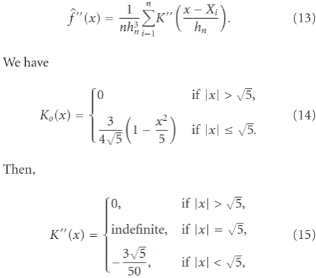
Figure1: Multimodal pdf estimated using optimal plug-in KDE and fast optimal plug-in KDE (power 6).
3.3. Estimation of simulated Gaussian mixture pdf
In this section, the following Gaussian distribution mixtures are considered.
3.3.1. Multimodal distribution
f(x)=π1fμ1,σ1(x) +π2fμ2,σ2(x) +π3fμ3,σ3(x) (21)
withμ1= −1, μ2=0, μ3=1, andσ1=0.5, σ2=0.3, σ3=
0.2, μi, andσ2
i are, respectively, the mean and the variance of
each distribution.
The a priori probabilitiesπ1, π2, andπ3are, respectively,
equal to 0.3, 0.35, and 0.35. The data size is 1000. Then, plug-in optimal KDE and fast plug-plug-in optimal KDE are applied. The two estimations are compared with the theoretical dis-tribution in the mean of MISE criterion which is computed for each case.
Figure 1 represents each of the KDE pdf estimations using both the fast plug-in algorithm (power 6 and power 4.5) and the classical plug-in algorithm for estimating the
Table2: MISE and variance of 100 simulations of the two studied KDE.
MISE∗10−4 Variance∗10−8
Plug-in optimal KDE 2.8 9.9
Fast plug-in optimal KDE 2.7 1.1
optimal bandwidth. It is clear that the convergence is not reached with the bandwidth selected by using the fast plug-in algorithm.
However, the power ofhnhas been adjusted experimen-tally.Figure 2clearly shows that the choice of 4.5 as a power value of hn in (20) instead of 6 enables the fast plug-in optimal KDE to give a pdf estimation as good as the classical plug-in optimal KDE. This result is corroborated by MISE values and their variance presented inTable 2.
Figure 3 plots the evolution of the MISE versus the sample size (100 iterations). The two curves are very close: the MISE, while having nearly the same values, are weaker, and tends toward 0 when the sample size is growing.
Table 3summarizes the MISE values and their variances: the difference between the estimations issued from the two plug-in KDE tends toward 0.
3.3.2. Bimodal distribution
The study of another example which includes a uniform distribution known for its estimation difficulties is proposed below:
f(x)=π1fμ,σ(x) +π2fa,b(x) (22)
with μ = 0.3 and σ = 0.2; μand σ are, respectively, the mean and the variance of the Gaussian distribution. The parameters of the uniform distribution are a = −0.3 and
b=0.2.
The a priori probabilities π1 and π2 are, respectively,
0.75 for the Gaussian distribution and 0.25 for the uniform distribution. The sample size is 4000.
The results are the same as those obtained for the multi-modal distribution. As observed inFigure 4, the convergence is obtained with (20), that is, a power value of 4.5 forhn. The two KDE give close estimations of the pdf. The MISE and their variances confirm these observations (Table 4).
3.4. Complexity and convergence
For the plug-in optimal KDE algorithm, f and J(f) are estimated k times, where k is the number of iterations. k
−5 −4 −3 −2 −1 0 1 2 3 4 0
0.2 0.4 0.6
0.8 Fast optimal plug-in KDE
Theoretical pdf Estimated pdf
(a)
−5 −4 −3 −2 −1 0 1 2 3 4
0 0.2 0.4 0.6
0.8 Optimal plug-in KDE
Theoretical pdf Estimated pdf
(b)
Figure2: Estimation of simulated pdf using optimal plug-in KDE and fast optimal plug-in KDE (power 4.5).
Table3: Convergence of MISE and variance values versus sample size computed from 1000 simulations of the theoretical distribution using the two studied KDE.
Sample size 500 1000 1500 2000 2500 3000 3500 4000
Fast plug-in KDE 10
−4∗MISE 8.3 6.3 5.5 5.3 4.7 4.4 4.4 4.3
10−8∗variance 27.5 13.6 9.6 8.3 6.2 5.2 3.4 3.0
Plug-in KDE 10
−4∗MISE 8.5 6.4 5.6 5.3 4.7 4.5 4.4 4.3
10−8∗variance 26.7 13.0 7.8 7.4 4.3 4.3 3.2 3.0
500 1000 1500 2000 2500 3000 3500 4000 Sample size
3 4 5 6 7 8 9
×10−4
MISE
Plug-in KDE Fast plug-in KDE
Figure3: MISE estimated by plug-in optimal KDE and fast plug-in optimal KDE (power 4.5) versus the sample size.
Table4: MISE and variance of 100 simulations of the theoretical distribution using the two studied KDE.
MISE∗10−3 Variance∗10−6
Plug-in optimal
KDE 21.8 26.1
Fast plug-in optimal
KDE (power 4.5) 21.8 26.4
−01.5 −1 −0.5 0 0.5 1 1.5 2
1 2
3 Fast optimal plug-in KDE (power 6)
Theoretical pdf Estimated pdf
(a)
−01.5 −1 −0.5 0 0.5 1 1.5 2
1
2 Fast optimal plug-in KDE (power 4.5)
Theoretical pdf Estimated pdf
(b)
−01.5 −1 −0.5 0 0.5 1 1.5 2
1
2 Optimal plug-in KDE
Theoretical pdf Estimated pdf
(c)
Table5: Characteristics of the studied populations.
Population n π Dp
Sened 55 7.60471 −1.717
Testour 40 6.33846 −1.755
−4 −3 −2 −1 0 1 2 3 4
0 0.2 0.4
Estimation ofD-pdf with plug-in optimal KDE
(a)
−4 −3 −2 −1 0 1 2 3 4
0 0.2 0.4
Estimation ofD-pdf with fast plug-in optimal KDE
(b)
Figure5: Estimation of theD-pdf of Sened by optimal plug-in KDE and fast plug-in KDE.
resolution. The estimation off isO(2np), and the estimation ofJ(f) isO(2p). The complexity of this iterative algorithm is consequently O(2knp). In the fast plug-in optimal KDE algorithm,f is estimated only once. Thus, the computational cost of this algorithm is O(2p(k+n)). The value of k is small in comparison to the value ofn : kis around 5 and
ngenerally exceeds 500. It can, therefore, be neglected and the computational cost becomesO(2np).
4. ESTIMATION OF PDF OF TUNISIAN GENETIC PARAMETER
In this section, we are interested in the genetics of pop-ulations and more specifically in Tajima’s estimation of the pdf of the statistic D of Tajima. This is estimated in order to evaluate the neutrality of studied populations. The data are obtained by generating neutral populations, using parametersθandn[8]. Such parameters are computed from the sample data. The parameter θ is defined as equal to 4Nμ, Nbeing the effective population size,μthe mutations number per generation, andnis the sample size.
Several methods have been proposed to estimateθ. We can cite here the number of segregation sites S [9] and the average number of (pairwise) nucleotides differences between the DNA sequences, calledπ[10].
πgives a direct estimation ofθ, that is,E(π)=θ. On the other hand, we have θ = S/a1, where a1 =
n−1 i=1(1/i).
−4 −3 −2 −1 0 1 2 3 4
0 0.2 0.4
Estimation ofD-pdf with plug-in optimal KDE
(a)
−4 −3 −2 −1 0 1 2 3 4
0 0.2 0.4
Estimation ofD-pdf with fast plug-in optimal KDE
(b)
Figure6: Estimation of theD-pdf of Testour by optimal plug-in KDE and fast plug-in KDE.
The difference betweenSandπis the effect of selection.
Deleterious mutants are maintained in a population with low frequency. If some of the mutants observed have a low frequency,πmay not be the same asS/a1.
Tajima has proposed the following statistic:
D= d
V(d)
=π−S/a1
V(d)
. (23)
The mean and the variance of the statistic D are approximately 0 and 1, respectively. If the distribution ofD
is known, it is possible to use it in testing neutral mutation hypothesis. For this purpose, a computer simulation was conducted [8] using S and π parameters computed from the actual data. The value of Dobtained from the studied population sample using (23) is calledDp. P[D < Dp] must be higher than 0.02 for declaring the population as neutral with a first-kind riskαequals to 5%.
The characteristics of the considered populations are introduced inTable 5.
Pdf of theoretical neutral distributions ofDare estimated by using the two plug-in optimal KDE studied in this paper: the plug-in optimal KDE and the fast plug-in optimal KDE. It is noticed that there are no differences between the two estimations (Figures5and6).
For a better estimation of the neutrality of the studied populations, we propose to compute a mean value of
P[D < Dp] deducted from 100 simulations of theoretical neutral populations. The obtained results are presented in
Table 6.
Table6: Mean values ofP[D < Dp] obtained from the two optimal plug-in KDE studied.
P[D < Dp] (Mean value)
Population Plug-in optimal KDE Fast plug-in optimal KDE
Sened 21.3∗10−3 21.4∗10−3
Testour 18.3∗10−3 18.4∗10−3
fast optimal KDE relatively to the optimal KDE concerns particularly the computational cost.
5. CONCLUSIONS
In this paper, we have presented a fast version of the plug-in algorithm which estimates the optimal KDE bandwidth as well as the classical plug-in algorithm. Such a method is based on the optimal kernel which is directly derived without taking the indefinite points into account. The convergence in the MISE sense is obtained with less complexity.
The entity noticed byJ(f) which represents the integral of the second-order derivative of the pdf is approximated analytically at each iteration in order to tend to the optimal bandwidth. However, the mathematical expression computed analytically (19) gives an incorrect estimation of the tested pdf. The value of the power ofhnwas, therefore, experimentally adjusted to 4.5. The efficiency of this fast algorithm was tested on several simulations of multimodal densities which are known for being difficult cases in the mean of estimation problem, and the proposed algorithm allows estimation comparable to the plug-in optimal KDE in the MISE sense with an improvement of the computational cost.
In the field of genetic population, this fast algorithm allows a better estimation of the neutrality of studied populations in the computational cost sense, especially if this neutrality is not robust (P[D < Dp] ≈ 0.02). The computation of a mean value of this probability needs a large computational time. The use of the fast plug-in optimal KDE provides an improvement of the computational cost without any loss of quality of results studied.
In fact, several applications could be concerned by the proposed fast algorithm. The estimation of the probability error for the CDMA communication systems should be mentioned as it will be considered in future work. The generalization to the multivariate case will also be dealt with, in addition to the consideration of densities confined to a bounded support [3,11,12] in order to study the same idea for the diffeomorphism KDE.
APPENDIX
MSE=E fn−f 2=E f2 n
+f2−2f E fn,
E fn−f 2=E f2 n
−E fn2+E fn2+f2−2f E fn,
E fn−f 2=var fn+f −E fn2.
(A.1)
Let us compute the variance of fn for a kernel density estimator assuming that the kernel K is an even regular function with unit variance and zero mean:
var fn=var
1
nhn n
i=1 K
x−Xi hn
,
var fn= 1
n2h2 n
var
n
i=1 K
x−Xi hn
,
var fn= n
n2h2 n
var
K
x−X1 hn = 1 nh2 n var K
x−X1 hn
,
var fn= 1
nh2 n E K2
x−X1 hn − E K
x−X1 hn
2
,
var fn= 1
nh2 n
K2
x−y
hn
f(y)d y
−
K
x−y hn
f(y)d y
2 .
(A.2)
Let us consider the following change of variable:u= ((x−
y)/hn),
var fn= 1
nh2 n
K2(u)fx−hnuhndu
−
K(u)fx−hnuhndu
2
,
var fn= 1
nhn
K2(u)fx−hnudu
−1
n
K(u)fx−hnudu
2 .
(A.3)
Secondly, we are interested in the development of (f −
E[fn] )2,
E fn=E
1
nhn n
i=1 K
x−Xi hn
,
E fn= 1
nhnE
n
i=1 K
x−Xi hn
,
E fn= n
nhnE
K
x−X1 hn
,
E fn= 1
hn
K
x−y
hn
f(y)d y.
Let us consider the following change of variableu=((x−
y)/hn),
E fn= 1
hn
K(u)fx−uhnhndu
=
K(u)fx−uhndu,
f −E fn2=E fn−f2
=
K(u)fx−uhndu−
K(u)f(x)du
2
,
E fn−f2=
K(u)fx−uhn−f(x)du
2 .
(A.5) Using (A.3) and (A.5), we have
E fn−f 2= 1
nhn
K2(u)fx−hnudu
+
K(u)fx−uhn−f(x)du
2
−1
n
K(u)fx−hnudu
2
=An(x) +Bn(x)−Cn(x)
(A.6) with
An(x)= 1
nhn
K2(u)fx−hnudu,
Bn(x)=
K(u)fx−uhn−f(x)du
2
,
Cn(x)=1
n
K(u)fx−hnudu
2 .
(A.7)
By introducing the following Taylor expansion,
fx−hnu
= f(x)−hnu f(x) +u
2
2h
2
nf(x)− u3h3
n
6 f
(3)x−θhnu,
(A.8) where 0< θ <1, An(x) andBn(x) can be approximated by
An(x)≈ f(x)
nhn
+∞
−∞K
2(u)du,
Bn(x)≈
−f(x)h4n
+∞
−∞uK(u)du
+ f
(x)
2 h
2 n
+∞
−∞u
2K(u)du
2
,
Cn(x)≈ f2(x)
n .
(A.9)
By considering only even kernels with unit variance and zero mean,
Bn(x)≈ f
2
4 h
4 n,
MISE= +∞
−∞
An(x) +Bn(x)−Cn(x)dx.
(A.10)
By using the following notations:
M(K)= +∞
−∞K
2(u)du, J(f)=
+∞
−∞
f(x)2dx, (A.11) where f is the second derivative of f; MISE can be approximated byΔ(hn); the Taylor expansion. Then,
MISE≈Δhn=M(K)
nhn + J(f)h4
n
4 . (A.12)
REFERENCES
[1] H. Oja, “On location, scale, skewness and kurtosis of univari-ate distribution,”Scandinavian Journal of Statistics, vol. 8, no. 2, pp. 164–168, 1981.
[2] A. W. Bowman and A. Azzalini,Applied Smoothing Techniques for Data Analysis, Oxford University Press, Oxford, UK, 1997. [3] P. Hall, “Comparison of two orthogonal series methods of estimating a density and its derivatives on interval,”Journal of Multivariate Analysis, vol. 12, no. 3, pp. 432–449, 1982. [4] B. W. Silverman, Density Estimation for Statistics and Data
Analysis, Chapman & Hall, London, UK, 1986.
[5] M. Rozenblatt, “Remarks on some non-parametric estimates of a density function,”Annals of Mathematical Statistics, vol. 27, no. 3, pp. 832–837, 1956.
[6] E. Parzen, “On estimation of a probability density function and mode,”Annals of mathematical statistics, vol. 33, no. 3, pp. 1065–1076, 1962.
[7] M. C. Jones, J. S. Marron, and S. J. Sheather, “A brief survey of bandwidth selection for density estimation,”Journal of the American Statistical Association, vol. 91, no. 433, pp. 401–407, 1996.
[8] F. Tajima, “Statistical method for testing the neutral mutation hypothesis by DNA polymorphism,”Genetics, vol. 123, no. 3, pp. 585–595, 1989.
[9] G. A. Watterson, “On the number of segregating sites in genet-ical models without recombination,” Theoretical Population Biology, vol. 7, no. 2, pp. 256–276, 1975.
[10] F. Tajima, “Evolutionary relationship of DNA sequences in finite populations,” Genetics, vol. 105, no. 2, pp. 437–460, 1983.
[11] S. Saoudi, A. Hillion, and F. Ghorbel, “Non-parametric probability density function estimation on a bounded sup-port: applications to shape classification and speech coding,”
Applied Stochastic Models and Data Analysis, vol. 10, no. 3, pp. 215–231, 1994.