Spatially Resolved Star Formation in Cosmological Zoom-in Simulations: Understanding the Role of Feedback in Scaling Relations

(1)

Spatially Resolved Star Formation in Cosmological

Zoom-in Simulations: Understanding the Role of

Feedback in Scaling Relations

Thesis by

Matthew Edward Orr

In Partial Fulfillment of the Requirements for the

Degree of

Doctor of Philosophy

CALIFORNIA INSTITUTE OF TECHNOLOGY

Pasadena, California

2019

(2)

Matthew Edward Orr ORCID: 0000-0003-1053-3081

(3)

ACKNOWLEDGEMENTS

I have no doubts that I will look back fondly on graduate school as a formative

period in becoming a scientist, mentor, some degree of leader, and, in steps, a better

person. I think that it would be laughable to consider any of that happening on its

own without the host of family, friends, mentors, and advisors I have had supporting

me over the past five years in graduate school, and for the twenty-two years before

that.

First, I want to thank my late father, Steven Robert Orr, for all his encouragement

and council over the years. When I was torn over whether to pursue astrophysics

or “something more practical”, his wisdom was my guide. When I think about the

man I have become, and the man that I want to be, I will always think of my Dad. I

have missed him in my time at Caltech. And yet, I am sure I could not have finished

a doctorate without him.

I could not saythank youenough to my advisor, Phil Hopkins. Between his patience,

guidance, in matters both scientific and not, and, of course, funding, I could not

have become the astrophysicist I am today. I am indebted to him for shepherding me

through my graduate years. In a similar vein, I am not sure any of my work would

be half as good without Chris Hayward. Through both being a great mentor and his

help in keeping my manuscripts from being unreadable messes, Chris kept me from

becoming a mess an uncountable number of times during my doctorate.

Needless to say that my time at Caltech would have been very different without

the early guidance of Jorge Pineda & Paul Goldsmith. They both showed me how

fascinating and fun astrophysics is, and helped me find my way back to astrophysics

in a time of doubt and uncertainty. I am forever grateful for all their help and

guidance over the years, and am glad to call them friends.

I am grateful for my friends, and all that time spent not in my office in Cahill, who

kept me sane over the years. In particular, the great sports dynasties ofthe Fightin’ Pinecones and the Coors Party Train Disaster, the perfectly adequate athleticism

of which were always an inspiration. My once-roommate and always-great travel

companion, Vatsal Jhalani, and the men of Glen Arbor and Layton St., John Rodli,

Phil Montoya, Kyle Mickelson, Connor McCann, and Kirk Nilsson, all are owed

particular thanks, for putting up with my odd schedule and hobbies, and for being

(4)

Special thanks to my friends from Cahill, Ivanna A. Escala, Denise Schmitz, Gina

Duggan, Dr. Allison Strom, and Dr. Alicia Lanz, who all taught me more than

anyone about how to navigate graduate school, be an astrophysicist, and how to

run a Graduate Student Council. I look forward to visiting with them at many

workshops, conferences, and symposia in the years to come.

Though not in Cahill, my dear friends Elise Post, Joe Bowkett, Brenden Roberts, Phil

Jahelka, Thom Bohdanowicz, Mali Zhang, Leah Sabbeth, Soichi Hirokawa, Julia

Levy, Jeremy Moskovitz, Emma Young, and many more all deserve many many

thanks, for the adventures, the variousPineconesvictories, and their fellowship in

my time at the California Institute of Technology.

Of course, thank you to my family, who put up with me all these years. I would

not have gotten where I am today without my mother, Cheryl Orr, or my brother,

William Orr. They have been both voices of reason, and great sources of inspiration

over the years. My grandparents too, Thelma and the Rev. Prof. Dr. John Berk Orr,

have been both the best grandparents anyone could ask for, and great sages on the

academic path. I also owe Belle Berk Orr, ever the loyal companion, many treats

and walks. Lastly, I must thank Emma Reinhart for being a positive, caring partner

through these stressful times. Without her, graduate school would have been a far

(5)

ABSTRACT

To understand the night sky is to understand how galaxies form their stars.

Cos-mological zoom-in simulations, which self-consistently evolve a small number of

galaxies at very high resolution by embedding them within a fully cosmological

box, have evolved over the last 25 years to a level of realism where they can begin

to tackle questions of spatially resolved star formation within galaxies. Whereas a

decade ago simulations faced difficulty in matching even global properties of

ob-served galaxies (e.g., the ratio of stellar mass to total halo mass), the state of the

art is now able to meaningfully recover resolved quantities in galaxies that were not

put into the simulations by hand (e.g., the Kennicutt-Schmidt star formation scaling

relation).

The research presented in this thesis seeks to understand how the physics of star

formation and stellar feedback from massive stars shape and regulate the interstellar

medium (ISM)withingalaxies. Particularly, the focus lies on the scale of the largest

coherent structures in galaxies–the disk scale height. To explore these physics,

the cosmological zoom-in simulations of the Feedback in Realistic Environments

(FIRE) project (Hopkins, Kereš, et al., 2014; Hopkins, Wetzel, et al., 2018) are

used.

The chapters of this thesis explore various topics in spatially resolved star formation,

including: the Kennicutt-Schmidt relation (Schmidt, 1959; Kennicutt, 1998), an

empirical relation between gas surface density and star formation rates, in the

FIRE-1 simulations (Orr, Hayward, Hopkins, et al., 20FIRE-18), including an examination what

set the extent of the star-forming disks in the simulations (i.e., what causes star

formation tofireup in the outskirts); an examination of the observational method of

analyzing stacks of galaxy observations, finding that temporal variations in spatially

resolved star formation rateswithinindividual galaxies were more than enough to

bias stacking analysis of star formation rate profiles; a semi-analytic model of

non-equilibrium star formation rates, relating to the competition between the feedback

timescale associated with star formation and local dynamical times (Orr, Hayward,

and Hopkins, 2019), which explores this as a source of scatter in the

Kennicutt-Schmidt relation; and finally, investigating how gas velocity dispersions and star

formation rates relate in FIRE-2 Milky Way-mass disk galaxies, exploring whether

or not feedback is primarily driving the velocity dispersions in galaxies, and how

(6)

PUBLISHED CONTENT AND CONTRIBUTIONS

Orr, M. E., Hayward, C. C., & Hopkins, P. F. (2019) Monthly Notices of the Royal Astronomical Society 486, 4724

DOI:10.1093/mnras/sty1241

MEO conceived the project, conducted the science analysis and wrote the manuscript.

Orr, M. E., Hayward, C. C., Hopkins, P. F., et al. (2018) Monthly Notices of the Royal Astronomical Society 478, 3653

DOI:10.1093/mnras/sty1241

PFH and MEO conceived the project. MEO conducted the science analysis and wrote the manuscript.

Orr, M. E., Hayward, C. C., Nelson, E. J., et al. (2017) Astrophysical Journal 849, L2

DOI:10.3847/2041-8213/aa8f93

MEO and CCH conceived the project, coordinating with EJN. MEO conducted the science analysis, and wrote the manuscript.

Orr, M. E., Pineda, J. L., & Goldsmith, P. F. (2014) Astrophysical Journal 795, 26

DOI:10.1088/0004-637X/795/1/26

(7)

LIST OF ILLUSTRATIONS

Number Page

1.1 Galaxies in the (simulated) cosmic web . . . 6

1.2 Observed Kennicutt-Schmidt Relation circa 2012 . . . 11

1.3 Defining velocity dispersions in observations and theory . . . 12

2.1 Example of a spatially resolved galaxy map from FIRE . . . 21

2.2 Spatially resolved Kennicutt-Schmidt relation in FIRE for various gas and star formation tracers . . . 27

2.3 Spatially resolved Elmegreen-Silk relation in FIRE for various gas and star formation tracers . . . 35

2.4 Spatially resolved Kennicutt-Schmidt relation in FIRE with a 100 Myr-averaged SFR tracer . . . 36

2.5 Pixel size dependence of FIRE molecular Kennicutt-Schmidt relation 38 2.6 Redshift dependence of spatially resolved Elmegreen-Silk relation in FIRE . . . 39

2.7 Redshift and metallicity dependences of spatially resolved Kennicutt-Schmidt relation in FIRE . . . 40

2.8 Metallicity dependence of star formation rate in FIRE . . . 41

2.9 Dynamical time dependence of star formation rate in FIRE . . . 42

2.10 Gravitational instabilities vs. self-shielding thresholds for Star for-mation in FIRE . . . 48

2.11 Physics tests in simulation restarts for star formation thresholds . . . 49

2.12 Star formation prescription parameter study for self-regulation in FIRE galaxies . . . 58

2.13 Evolution of gas density CDF with different star formation prescrip-tions in FIRE . . . 59

2.14 Comparison in Kennicutt-Schmidt of several proxies for tracing molec-ular gas in FIRE . . . 61

2.15 Spatially resolved cold & dense gas fraction in FIRE compared to theory . . . 62

(9)

3.1 Comparison between individual SFR profiles and stacked SFR

pro-files at z ≈1.4 in FIRE galaxies . . . 76 3.2 Evolution of star formation main sequence for several FIRE galaxies

between z =1.5−0.7 . . . 77 3.3 Stacked SFR and gas profiles in FIRE galaxies above and below the

main sequence . . . 78

3.4 SFR profiles form12vabove and below the main sequence . . . 79

4.1 Evolution of model SFR and velocity dispersion in a fiducial ISM patch100

4.2 Kennicutt-Schmidt, sSFR– ˜Qgas, and velocity dispersion relations of

fiducial model across Σgas . . . 101

4.3 Effects on model normalization and scatter of variations in strength,

delay until, and duration of feedback . . . 104

4.4 Effects on model normalization and scatter of variations in star

for-mation prescription . . . 105

4.5 Mock galaxies produced by the model on various star formation

scaling relations . . . 110

4.6 Effect of varying the SFR averaging period on model predictions . . . 119

5.1 Spatially resolved maps of star formation and gas quantities in the

FIRE-2 galaxies (m12b-m12i) . . . 133

5.2 Spatially resolved maps of star formation and gas quantities in the

FIRE-2 galaxies (m12m-m12w) . . . 134

5.3 Gas velocity dispersion–SFR relation in individual FIRE-2 galaxies . 135

5.4 Spatially resolved FIRE-2 spiral galaxy gas velocity dispersion–SFR

relation for various ISM components and SFR tracers . . . 137

5.5 Gas velocity dispersions as a function of gaseous and stellar surface

densities in FIRE-2 galaxies . . . 139

5.6 Gas properties across velocity dispersion–SFR relation in FIRE-2

galaxies . . . 141

5.7 Instantaneous and 100 Myr SFRs across velocity dispersion–SFR

relation (10 Myr avg.) in FIRE-2 galaxies . . . 144

5.8 Outflow ability on different timescales bounds for velocity dispersion–

SFR relation in simulations . . . 146

5.9 Depletion times across velocity dispersion–SFR relation in FIRE-2

galaxies . . . 148

5.10 Spatially resolved depletion times and sSFRs in FIRE-2 galaxies as

(10)

5.11 Gas fractions, outflow-prone fractions, and star formation burst

fac-tors in FIRE-2 galaxies as a function of current and required (for ISM

stability) gas velocity dispersions . . . 151

5.12 Imprint of bursty star formation in depletion time–Toomre-Q relation

in FIRE-2 galaxies . . . 152

5.13 Velocity dispersion predictions from ISM/SF models compared to

FIRE-2 galaxies . . . 156

6.1 Spatially resolved Kennicutt-Schmidt relation in a FIRE-2 Milky

Way-mass spiral galaxy . . . 170

(11)

LIST OF TABLES

Number Page

3.1 Simulation Properties at z= 1 . . . 80

4.1 Summary of variables used in this chapter . . . 92

4.2 Fiducial Model Parameters and Disk Conditions . . . 98

4.3 Properties of Mock Galaxies for Figure 4.5 . . . 109

(12)

FORWARD

At the end of graduate school, I have found that it was a rather circuitous route to get

here. It was not a given that I would become a theoretical astrophysicist in the least.

Had I been asked what I was going to be in the Fall of 2010, my response would

be been, without hesitation, a “Rocket Scientist”. Over the ensuing decade, I kept

the scientist part, but moved in half-steps from the practical, albeit highly esoteric,

work of astronautical engineering towards astrophysics. This thesis represents the

culmination of that journey from engineer to scientist. I think, however, that the

reader would enjoy knowing the fall from grace, required to make a theorist, that

took place.

Arriving at the University of Southern California (USC) for college, a whole

twenty-five-minute drive away from home in leafy La Cañada Flintridge, California, I was

excited to study astronautical engineering. There was not a tremendous amount of

thought that had gone into the decision. I feel now that I had inexorably fell into

it- after all, I had grown up with countless friends whose parents had calculated

launch windows for Mars probes or designed high-gain antennas for deep space

missions, visited Caltech’s NASA Jet Propulsions Laboratory (JPL) on what were

effectively annual school-sponsored scientific pilgrimages, and somehow had gotten

to building air-pressurized water rockets from parts cobbled together from soda

bottles and OSH/Harbor Freight tools. Rockets were cool, space was captivating,

and of course I was going to major in astronautics.

I was not a great student in high school. But I did enjoy my science and math

classes. My chemistry and physics classes were the most interesting. I had taken

well to learning that the world had rules, and by following them you could build

neat things. Reflecting back on it, I am surprised that I did not fall in with the kids

in the robotics club, jumpstarting my whole arc through engineering. I was more

interested in hanging out with my friends, playing videogames, hosting frequent

LAN parties, and generally just being a teenager. It was probably better for me.

In college, however, I was a great student, at least by my standards. I just loved

my first couple of courses, especially ASTE101 with Dr. Anthony Pancotti. I

was calculating orbits for imaginary missions to Ganymede, learning about rocket

staging and the different kinds of rocket motors. That class lit a fire under me that

(13)

Air Force Research Labs’ Collaborative High Altitude Flow Facility (CHAFF) on

campus in the Rapp Research Building (RRB). It would be my first experience with

research, and arguably the most important. I spent three years there, with (the future

Dr.) Matthew Gilpin, trying to melt Boron with the Sun and develop far-out in-space

propulsion concepts. I do not think any other person, or experience, went so far to

convince me that research was what I wanted to do in life.

During this time, I fell into the USC Rocket Propulsion Lab (RPL)1also housed in

RRB. Though CHAFF may have shaped me into a researcher, “rocket lab” gave me

a family at college in people like Julia Levy and Turner Topping, and taught me that

I could build anything I wanted, provided that there was some scrap material lying

around, and the lathe and mill were powered. Under Bill Murray (III) and Alec

Leverette, the first two years of USC were a whirlwind of trips to the deserts near

and far, late nights getting things unstuck or laid-up, and seeing some incredible

flight vehicles go up2. Though I would leave rocket lab in my junior year, the friends

I made and the things I learned would stick with me for the rest of college, and my

life.

Sophomore and junior years, I had decided that my technical electives for

astro-nautical engineering would be astronomy courses. I had taken the honors series of

freshman physics courses with Dr. Gene Bickers, who had really opened my eyes

to how enjoyable and varied the topics of physics could be. So, going through a

course on the solar system, and one on astrophysics, I was hooked. I got mixed up

doing helioseismology work with Dr. Ed Rhodes at the Mt. Wilson Observatory

(the 60’ solar tower), and that was really the first astronomy work that I did. I spent

the summer between my sophomore and junior years variously in CHAFF and up

Mt. Wilson. On the mountain, I was learning Bash, running the dome and its

instruments, and taking long naps.

Around this time, I had begun to lose faith in the idea that I wanted a job in aerospace.

My friends from rocket lab were graduating, and the jobs they got terrified me. My

friends had to know their stuff day in and day out, and not fly by the seat of their

pants from one project to the next like I had been doing in CHAFF and at Mt.

Wilson. But I was not quite ready to abandon engineering altogether. I had it in my

mind that I needed a “practical degree”. And so, instead of going for astronomy, I

took the half-step to physics (with an astronomy minor).

1_{This name was indeed a joke on NASA’s JPL, since the founding students had thought that the} “Jet” part was a bit disingenuous.

(14)

Late in my junior year at USC, I realized that it was rather hard to get a degree in

both engineering and physics at the same time in four years. After much agonizing,

but with my father’s encouragement, I dropped my astronautics degree3: I was committed. I wanted to go to graduate school in physics, or maybe astronomy.

The next summer, I got an internship at JPL, with Drs. Paul Goldsmith and Jorge

Pineda studying the Taurus molecular cloud. I learned more physics of the

inter-stellar medium that summer than I ever have since. It also required me to actually

learn how to code, and write a scientific paper4. I got to walk the lab in thought, and

watch second-string rovers practice on dusty mounds of rock in the Arroyo Seco. It

was just great for someone dipping their toes into theory research.

Returning to campus in my last year of undergrad, I somehow convinced myself

that though I loved physics, especially astrophysics, I needed to do something

“practical”. So I threw myself at nanophotonics. Sure that this was what I was

going to do in graduate school, I took an EE course on the subject, wrote up an

NSF graduate fellowship proposal on it, and applied to every graduate school as an

applied physicist. I had never set foot in a nanophotonics lab, much less an optics

lab. Much to my surprise, I got into Caltech’s Applied Physics graduate program

amongst other schools.

All the prospective graduate school visits during my senior spring term excited me

to no end. Though I look back increasingly fondly on my time at USC now, in the

moment I was very happy to be ‘called up to the majors’ in terms of the schools I

was considering for my Ph.D. After much debate with my partner at the time, we

settled on going to Caltech together for our Ph.Ds.

Graduating USC that May, with an NSF Graduate Research Fellowship in hand (for

a proposed nanophotonics project), and headed up the 110 to Pasadena in the fall,

I was on top of the world. After graduation, we headed off on a family trip, which

would then become a trip with friends, across Northern and Central Europe. Two

weeks into the adventure, I said farewell to my family in Copenhagen. I also said

goodbye to my father for the last time, but I did not know it then. As we landed in

Boston for the last leg of the trip, a weeklong visit in Rhode Island, I learned that

my father had unexpectedly passed away during the night while I was in the air.

3

With all my newfound time, I took a table tennis course, and a ballroom dance class with my college girlfriend.

4

(15)

The fallout would cover much of the first two years of graduate school. Arriving at

Caltech that fall, I found myself in misery. The light that I had from undergrad was

snuffed out, and I struggled through courses. My relationship fell apart. On top of

all this, I realized that I truly hated cleanrooms. They are cold, inhospitably dry,

without Wi-Fi or cell service several floors underground, and have the most awful

spectrum of yellow lights. This meant, amongst other things, that nanophotonics

was not for me. I was adrift in the sea of graduate school.

With some encouragement, I reached out to my old mentors at JPL, inquiring if they

knew anyone down on campus that was doing astronomy. It just so happened that

Dr. Pineda was co-leading a Keck Institute for Space Sciences (KISS) workshop

on “Bridging the Gap: Observations and Theory of Star Formation Meet on Large

and Small Scales” the next month. Jorge invited me to come to the whiskey hour at

the workshop, and meet the people attending. There, I first met my Ph.D. advisor,

Dr. Philip F. Hopkins, whom I later reached out to so as to arrange a chat about his

research; and of course, whether or not I could do a small project with him.

In the coming weeks and months, that small project became my study of the spatially

resolved Kennicutt-Schmidt relation in the FIRE (Feedback in Realistic

Environ-ments) simulations, which would take up a large fraction of the early years of

graduate school (Orr, Hayward, et al., 2018). Slowly, I dragged my way back to

a healthy mindset. In fits and starts5, I learned more about the simulations, how

to work with them, and how to run them. I even switched from applied physics to

physics, mostly symbolically, but with the (false) hope that it would save me taking

a few courses. I embraced being a theorist, with only small fits of rebellion: I got

certified in the machine shop, which I maintain makes me the first theorist in physics

in a very long time to do so, and took up fine woodworking.

The rest of this thesis tells the story from there of the burgeoning theorist, who was

once an engineer and still a bit of one at heart.

Matthew Orr

May 2019

Caltech, Pasadena, CA

(16)

C h a p t e r 1

INTRODUCTION

The Big Picture: Galaxies and Their Cosmological Context

Across the vast majority of the history of the Universe, gravity has been the

dom-inant force. That hegemony began during the Dark Age of the Universe, between

decoupling approximately 400,000 years after the Big Bang, which gave us the

Cos-mic Microwave Background, and the time of the first stars, around 400 Myr into the

history of the Universe (Abel et al., 1998; Bromm et al., 1999). Recent observations

suggest that we may indeed be living through interesting times (Riess, Filippenko,

et al., 1998): the presumed largest energy component of the Universe, the source of

which remains a theoretical mystery, Dark Energy, is now taking the mantle from

gravity, causing the expansion of the Universe to accelerate, rather than continue to

slow. Gravity held the crown for about 13.3 Gyr.

In this time, gravity worked towards a singular purpose: collapsing structures on

scales large and small, amplifying the initial density perturbations of the Universe

handed down shortly after the Big Bang. This is a hierarchical process, where

the largest structures begin to collapse first, with structures within them beginning

to condense thereafter in a nested fashion. And so, a knotted web of (dark and

baryonic1) matter begins to collapse initially (Abel et al., 1998). From those

cos-mological scales, gas and dark matter is drawn into the densest regions. These are

the seeds of galaxies, that grow through cosmic time as gas and dark matter fall

into them, and gas is processed into stars (Silk, 1983; Bromm et al., 1999; Schaye

et al., 2015). Figure 1.1 shows a slice of a large-box simulation, in which galaxies

have formed and evolved in the filamentary matter overdensities in line with this

framework of hierarchical structure formation. Through the 1970s, much of our

understanding of galaxy evolution and populations stopped with the formation of

structure in the Universe, with a failure to understand why the galaxy mass function

today failed to match the self-similar solution of hierarchical collapse (Press et al.,

1974).

The fields of galaxy formation and evolution have experienced a renaissance in

(17)

(18)

the last two decades, as cosmologists pinned down the geometry and relative

com-position of the Universe following the careful work of the Wilkinson Microwave Anisotropy ProbeandPlancksatellite missions, combined with work on the

distance-redshift relation from Type Ia SNe, abundances and clustering of galaxies (e.g.,

baryon acoustic oscillations), and constraints on the present expansion rate of the

Universe (Hubble parameter H0) (Hinshaw et al., 2013; Planck Collaboration et al.,

2016; Riess, Macri, et al., 2016). The remaining uncertainties in the fundamental

cosmological parameters, for the purposes of understanding galaxy formation and

evolution, are largely inconsequential.

Baryons Don’t Just Sit There: Physics in Galaxies

Considering the whole volume of the Universe, gravity has ruled supreme

on-average. There are and have always been, however, pockets of resistance. Baryonic

matter fought back, and as in the cases of supernovae, sometimes quite vigorously.

So, in order to understand the process of galaxy evolution on smaller scales than the

cosmological web, we need to follow the hierarchical collapse of dark matter and

baryons down to scales within galaxies. Here, gravity is not the only force involved,

and baryonic processes can greatly affect the dynamics of matter. Within galaxies,

physical mechanisms like photoionizing radiation, winds, and supernovae (together

broadly known as feedback), the majority of which are associated with recently

formed, massive stars, fight gravitational collapse on length-scales of kiloparsecs,

e.g., spiral arm scales, down to less than a parsec, e.g., clumps within molecular

cloud complexes (Silk, 1997; Matzner, 2002; Shetty and Ostriker, 2008;

Faucher-Giguère et al., 2013; Stinson et al., 2013; Hopkins, Kereš, et al., 2014). This

involves a tremendous bridging of scales, from the largest coherent structures inside

of galaxies down to the photospheres massive stars providing the feedback, and

poses challenges to even the most imaginative theorist or competent numericist in

addressing with theory or simulations (Somerville et al., 2015).

Fundamentally, understanding how galaxies evolve in our Universe, beyond the

hierarchical collapse out of the cosmic web, reduces to the questions: How does

star formation proceed in galaxies, and what are the effects of star formation on

galaxies?

Sweating the Small Stuff: Grid-Scale Baryonic Physics in Simulations

Large-volume cosmological galaxy simulations, like Illustris or EAGLE

(19)

is to match population statistics of galaxies and cosmological structure on 100 Mpc

scales, necessarily treat the complex baryonic physics of galaxies at the grid scale,

in their cases, a few kiloparsecs. For dwarf galaxies, and galaxies at high redshift,

in which all of the star formation essentially occurs in a single star-forming region,

treating star formation as a single kpc-scale black/closed box is fairly successful at

predicting star formation histories and chemical abundances (Romano et al., 2013,

Escala et al. in prep.). All simulations ultimately require there to be rules applied at

the resolution scale, that account for the physics being simulated. These rules either

parameterize our ignorance through fudge factors, or use fits to the results of

simu-lations conducted on yet smaller scales. In these simusimu-lations, they tune their galaxy

physics to match galaxy-scale observations of things like Kennicutt-Schmidt or the

stellar mass–halo mass relations. The fudge factors in the large-box simulations

treat galaxies as black boxes that take in cosmological gas inflows, and

appropri-ately process it into a mass of stars and outflows. They can say very little about the

internal structure of galaxies themselves below a few kiloparsecs, or anything about

the process of star formation in molecular clouds.

Cosmological zoom-in simulations are situated between the large-box simulations

that attempt to model a non-negligible fraction of a Hubble volume, and

ultra-high-resolution simulations of individual star-forming clouds or single stars. In a real

sense, they were a missing link between the scales at which much of the consequential

physics in the interstellar medium (ISM) occurs and cosmological scales.

Zoom-in simulations take a mid-sized cosmological volume (a few dozen Mpc) that is

run with only dark matter (so called DMO, Dark Matter Only, simulations), in

which a desired dark matter halo forms, e.g., a 1012 M-massed halo in which a

Milky Way-like galaxy is likely to form. Once such a halo is found, the simulation

is then reset to an early time in the Universe (say, z ≈ 30), and populated with

baryonic matter at high resolution in the region (with a little breathing room) that

will collapse into that galaxy byz= 0. And so, these simulations are able to implant

highly resolved galaxies in their cosmological contexts to produce realistic artificial

galaxies (Hopkins, Kereš, et al., 2014; Wetzel et al., 2016; Hopkins, Wetzel, et al.,

2018). Zoom-in simulations are thus able to take the results of yet-more-highly

resolved simulations as rules at the resolution scale. For the FIRE-2 Milky Way

mass simulations, this scale is adaptive with the local gas density, but the minimum

force softening is now sub-parsec (Hopkins, Wetzel, et al., 2018). And their results

(20)

Questions That Keep You (Me) Up at Night About Star Formation

My research, during the course of my graduate studies, has focused on aspects of

star formation processes and their effectswithingalaxies, on kiloparsec (kpc) scales.

Several questions have arisen repeatedly in each of my published, and in progress,

works. In one form or another, they have been:

1. How does the local rate of star formation scale with the local properties of the

ISM within galaxies?

2. To what extent is star formation an active process versus a passive one, i.e.,

does star formation drive or regulate itself, and the ISM writ large, or is it

primarily subject to the whims of galaxy structure and ISM dynamics.

3. On what length- and timescales is it appropriate to ask these questions? On

kiloparsec-scales the ISM has turbulent momentum and an average density

which may inform, be affected by, or drive star formation on the timescale of

galactic dynamical times, but down at the parsec scale things are different.

Stellar evolution and the properties of the ISM matter only in the direct vicinity

of individual (or a few) stars. Scaling relations like Kennicutt-Schmidt are

simply not well defined on that spatial scale, or over timescales much shorter

than a galactic dynamical time.

These questions rake at the mystery of star formation in galaxies from several

directions: the empirical question of simply, what does star formation scale with;

questions of causality, what can or ought to be considered driving the evolution of

galaxies; and semantic arguments relating to what meaning star formation scaling

relations can be held to have under which circumstances (e.g., what is theefficiency

of star formation?).

This last question is particularly vexing, as observers rarely, perhaps only in the

star-forming regions in the nearest dwarf companions to the Milky Way, count up

young stellar objects to get star formation rates (SFRs). They measure fluxes in

different wavelength bands. These fluxes are then connected, through a chain of

reasoning with a sturdy physical basis, to the properties of the unresolved stellar

populations within spatially resolved regions of galaxies. And from this, an estimate

for the mass of young stars present (which, owing to their short lifetimes, must have

(21)

formation rates. But again, the issue often at hand is the fact that observers measure

something that is correlatedwith star formation, but not star formation itself; and

so, the door is open to ask when do those fluxes not mean what an astronomer thinks

they mean.

The issue of connecting what is observable, fluxes from the far reaches of the

Universe, with the “ground truths” of the conditions within galaxies, is not reserved

solely to star formation rates. The issues calibrating star formation rate tracers are

nearly one and the same with those calibrating tracers of dense2 gas in galaxies.

A theorist, however, has a perfect model universe. Galaxies are well defined. Star

formation rates are the rate at which stars form. And dense gas masses are the amount

of gas of at least some density in a galaxy. We have no Humean3uncertainty in our

knowledge of our models or simulations. Moreover, simultaneous ‘observations’ of

both the gaseous and stellar components of galaxies are easy4.

The Kennicutt-Schmidt (or is it Schmidt-Kennicutt?) Relation

At least since the work of Schmidt (1959), but definitely since that of Kennicutt

(1989), astronomers and astrophysicists have framed much of the star formation

process in galaxies, i.e., on scales > 100 pc, as having something to do with the Kennicutt-Schmidt (KS, or Schmidt-Kennicutt, SK) relation (Bigiel et al., 2008;

Leroy, Walter, Brinks, et al., 2008; Dib, 2011; Ostriker et al., 2011;

Faucher-Giguère et al., 2013; Leroy, Walter, Sandstrom, et al., 2013; Shetty, Kelly, et al.,

2014; Orr, Hayward, Hopkins, et al., 2018, among others). The Kennicutt-Schmidt

relation is just the relationship between the surface density in dust and gas in a

galaxy, and the surface density of star formation. Canonically, it was found by

Kennicutt (1998) to have a scaling of ˙Σ? ∝ Σ1.4

gas (see Figure 1.2). The exponent

of this power law, and any other dependencies on galaxy quantities like metallicity,

gas fraction, etc., depend to varying extents on the tracers compared between the

gas surface densities, e.g., only molecular vs. atomic hydrogen, and star formation

rates, e.g., Hα vs. UV fluxes, each having different averaging timescales (Bigiel et al., 2008; Leroy, Walter, Sandstrom, et al., 2013; Dib, Hony, et al., 2017; Orr,

Hayward, Hopkins, et al., 2018).

2

Dense, here, is quite diffuse in human terms. Throughout this thesis, dense gas is taken often to encompass any gas denser thannH=1 cm

−₃

(atoms of Hydrogen per cubic centimeter). 3

David Hume (1711–1776), Scottish philosopher, economist, and historian.A Treatise of Human

Nature (1739–1740).

4

(22)

(23)

Figure 1.3: Observers and theorists often refer to different things when discussing velocity dispersions. Observers (left panel) talk of linewidths in gas emission or absorption lines, then connected to conditions in the gas, whereas theorists (right panel) think of Gaussian velocity dispersions and gas scale heights in galaxies or clouds directly. Left panel figure taken from Orr, Pineda, et al. (2014). Reproduced with permission.

As a scaffold for understanding, and defining, star formation processes in galaxies,

the Kennicutt-Schmidt relation has helped astronomers address many aspects of star

formation in galaxies and continues to be an intense area of research, though these

days primarily beyond the first order, comparing the subdominant dependences

of, e.g., metallicity, gas fraction, etc., on the star formation rate (Leroy, Walter,

Sandstrom, et al., 2013; Orr, Hayward, Hopkins, et al., 2018; Gallagher et al.,

2018). Understandably, all of the proceeding chapters of this thesis relate to the

Kennicutt-Schmidt relation in some way or another.

Linewidths, Velocity Dispersions, and Turbulence, Oh My!

Observers and theorists often run in different circles. Unsurprisingly, their

vocabu-laries can be slightly different. When discussing velocity dispersions, observers are

often speaking in terms of linewidths of gas emission or absorption lines like, e.g.,

the CO J = 1 →0 or the CII2P3/2 →2 P1/2transitions (e.g., Combes et al., 1997;

Bolatto, Leroy, et al., 2008; Goldsmith et al., 2008; Pineda et al., 2010; Wilson et al.,

2011). In this case, line broadening effects, beyond intrinsic linewidths, arise from

thermal or dynamical properties of the gas along the line of sight that is emitting or

absorbing light from that atomic or molecular transition. From this, observers infer

(24)

are only on solid ground when talking about the thermal or dynamical state ofthat particular component of the ISM, which corresponds to that emission/absorption

line. Theorists, on the other hand, often think directly of the dynamical structure

of the gas, i.e., the true velocity dispersions of particles in a 1-D or 3-D sense

(e.g., Toomre, 1964; Dib, Bell, et al., 2006; Krumholz et al., 2016; Orr, Hayward,

and Hopkins, 2019). And often, careful modeling of which components would be

emitting or absorbing at particular transitions is not done.

This is leaving out entirely the difficulties of translating integrated intensities to total

gas masses, etc. For example, as of the time of writing this thesis, there continues

to exist a lively debate in the fields studying galaxy formation and evolution, star

formation, and the ISM about how to convert integrated line intensities of CO to

molecular gas masses in galaxies (see Bolatto, Wolfire, et al., 2013, for a recent

review).

So, there is a gulf between observations and theory, which one must be careful

to navigate when interpreting either observations, or forecasting observables from

simulations and models. Throughout this thesis, unless otherwise noted, I take the

velocity dispersions (σ) to mean true dispersions in velocity of gas in the pixels discussed, and not as linewidths, as I have not published any linewidth predictions

from the FIRE simulations. Conveniently, this means that those velocity dispersions

can, in the context of galaxy disks and supersonic turbulence, to be directly related

to the gas disk scale heights (though H ≈ σ/Ω, where Ωis the orbital dynamical time) and the local Mach number (M = σ/cs, wherecs is the local sound speed).

1.1 Thesis Outline

The chapters in this thesis assault the questions posed, from how does star formation

scale with environment to what its roles in galaxies are. All of these investigations,

using both the FIRE simulations and semi-analytic models, ask to what extent, and

on what scales, can we consider the scalings of star formation meaningful in some

sense. The thesis is organized as follows:

• Chapter 2: Adapted from Orr, Hayward, Hopkins, et al. (2018), this chapter

explores the Kennicutt-Schmidt relation in the original FIRE simulations

(Hopkins, Kereš, et al., 2014). At the time, these simulations were among

the most highly resolved (both spatially and by particle mass) cosmological

zoom-in simulations. This allowed us to investigate in great detail how

(25)

with observations. The chapter explores how well various scalings predict

the star formation in the simulations, and touches lightly on the question of

star formation’s role in galaxies more broadly. The work of this chapter,

particularly in understanding whatfires up star formation in the simulations,

resulted in a collaboration with the MaNGA survey, studying star formation

thresholds in galaxies using their spatially resolved data (Stark et al., 2018).

• Chapter 3: This chapter is taken from Orr, Hayward, Nelson, et al. (2017), and

is primarily a fairly specific critique of an oft-used observational technique,

stacking many similar images of different galaxies at high redshift, in order

to push down on signal-to-noise limits and be able to say something about

galaxy properties or outskirts at z & 1. It investigates stacked star formation

rate profiles in the FIRE galaxies at z ∼ 1, and follows the observational

techniques of Nelson et al. (2016). Specifically, this letter addresses the

resulting physical interpretations for galaxies at high redshift, and how one

must be careful to not bias their interpretations when taking cuts of galaxy

populations from scaling relations like the star formation main sequence.

• Chapter 4: Unlike the other chapters of this thesis, this entry is not a direct

application of the FIRE simulations, but rather a semi-analytic toy model of

time-dependent star formation in galaxy disks, borrowing from Orr, Hayward,

and Hopkins (2019). It, being an excursion from simulations into

semi-analytic models, investigates thedynamicalevolution of a feedback-regulation

model, closely related to the frameworks of both Ostriker et al. (2011) and

Faucher-Giguère et al. (2013). This chapter takes a more substantive stab

at the second question posed: what is the role of star formation in galaxy

disks? In an evasive answer, star formation is both a passive respondent

to the ambient conditions, and an active driver of the state of the gas in

galaxies. It responds to the local state of the ISM (set by, e.g., past star

formation, cosmological inflows, or galactic structure), and then moves to

bend its surroundings to its will through processes of stellar feedback. Like

the phoenix, star-forming regions rise from the ashes of their predecessors,

and die in a combustion of their own making (feedback, both as supernovae

and radiation pressure/winds), existing in galaxies in a continual cycle of

death and renewal. In a related fashion, this chapter addresses the question

of on what timescales does it make sense to consider something like the

(26)

• Chapter 5: This chapter consists of as-of-yet unpublished work using the

FIRE-2 simulations. These simulations are the successor to the FIRE

simu-lations, improving upon the numerics, mass resolution, and feedback physics

implemented in the original suite. Here, we explore the relationship between

the gas velocity dispersions, in both the neutral and cold and dense gas, and

the star formation rates on ∼kpc-scales within the FIRE Milky Way mass

spiral galaxies at late timesz .0.1. This work stabs at the first two questions posed: scalings for and the role of star formation with respect to the structure

of the ISM within galaxy disks. Only briefly does it become philosophical

about timescales of meaningfulness for star formation scalings. Particularly

interesting for observers, perhaps, is that the erstwhile flat distribution of

velocity dispersions in gas, for a ∼ 3 dex range in star formation rates,

be-lies a consistent structure of gas properties scaling with star formation rates.

Self-regulation appears to rule galaxy disks, their gas component demanding

marginal stability against gravitational fragmentation and collapse. Though

the gaseous disks of these disk galaxies remembers past star formation and

feedback, that memory becomes quite hazy when searching more than a single

galactic dynamical time back.

Together, this opus of work constitutes both the culmination of a little more than four

years of work with Phil Hopkins and the broader FIRE collaboration, and a coherent

effort in understanding star formation processes within galaxies on kiloparsec-scales,

from the perspective of cosmological zoom-in simulations and semi-analytic models.

References

Abel, T., Anninos, P., Norman, M. L., & Zhang, Y. (1998) ApJ 508, 518

Bigiel, F., Leroy, A., Walter, F., Brinks, E., de Blok, W. J. G., Madore, B., & Thornley, M. D. (2008) AJ 136, 2846

Bolatto, A. D., Leroy, A. K., Rosolowsky, E., Walter, F., & Blitz, L. (2008) ApJ 686, 948

Bolatto, A. D., Wolfire, M., & Leroy, A. K. (2013) ARA&A 51, 207

Bromm, V., Coppi, P. S., & Larson, R. B. (1999) ApJ 527, L5

Combes, F. & Becquaert, J.-F. (1997) A&A 326, 554

Dib, S. (2011) ApJ 737, L20, L20

(27)

Dib, S., Hony, S., & Blanc, G. (2017) MNRAS 469, 1521

Faucher-Giguère, C.-A., Quataert, E., & Hopkins, P. F. (2013) MNRAS 433, 1970

Gallagher, M. J. et al. (2018) ApJ 858, 90, 90

Goldsmith, P. F., Heyer, M., Narayanan, G., Snell, R., Li, D., & Brunt, C. (2008) ApJ 680, 428

Hinshaw, G. et al. (2013) ApJS 208, 19, 19

Hopkins, P. F., Kereš, D., Oñorbe, J., Faucher-Giguère, C.-A., Quataert, E., Murray, N., & Bullock, J. S. (2014) MNRAS 445, 581

Hopkins, P. F., Wetzel, A., et al. (2018) MNRAS 480, 800

Kennicutt Jr., R. C. (1989) ApJ 344, 685

– (1998) ApJ 498, 541

Kennicutt, R. C. & Evans, N. J. (2012) ARA&A 50, 531

Krumholz, M. R. & Burkhart, B. (2016) MNRAS 458, 1671

Leroy, A. K., Walter, F., Brinks, E., Bigiel, F., de Blok, W. J. G., Madore, B., & Thornley, M. D. (2008) AJ 136, 2782

Leroy, A. K., Walter, F., Sandstrom, K., et al. (2013) AJ 146, 19, 19

Matzner, C. D. (2002) ApJ 566, 302

Nelson, E. J. et al. (2016) ApJ 828, 27, 27

Orr, M. E., Hayward, C. C., & Hopkins, P. F. (2019) MNRAS 486, 4724

Orr, M. E., Hayward, C. C., Hopkins, P. F., et al. (2018) MNRAS 478, 3653

Orr, M. E., Hayward, C. C., Nelson, E. J., et al. (2017) ApJ 849, L2

Orr, M. E., Pineda, J. L., & Goldsmith, P. F. (2014) ApJ 795, 26

Ostriker, E. C. & Shetty, R. (2011) ApJ 731, 41, 41

Pillepich, A. et al. (2018) MNRAS 473, 4077

Pineda, J. L., Goldsmith, P. F., Chapman, N., Snell, R. L., Li, D., Cambrésy, L., & Brunt, C. (2010) ApJ 721, 686

Planck Collaboration et al. (2016) A&A 594, A13, A13

Press, W. H. & Schechter, P. (1974) ApJ 187, 425

Riess, A. G., Filippenko, A. V., et al. (1998) AJ 116, 1009

Riess, A. G., Macri, L. M., et al. (2016) ApJ 826, 56, 56

Romano, D. & Starkenburg, E. (2013) MNRAS 434, 471

(28)

Schmidt, M. (1959) ApJ 129, 243

Shetty, R., Kelly, B. C., et al. (2014) MNRAS 437, L61

Shetty, R. & Ostriker, E. C. (2008) ApJ 684, 978

Silk, J. (1983) MNRAS 205, 705

– (1997) ApJ 481, 703

Somerville, R. S. & Davé, R. (2015) ARA&A 53, 51

Stark, D. V. et al. (2018) MNRAS 474, 2323

Stinson, G. S., Brook, C., Macciò, A. V., Wadsley, J., Quinn, T. R., & Couchman, H. M. P. (2013) MNRAS 428, 129

Toomre, A. (1964) ApJ 139, 1217

Vogelsberger, M. et al. (2014) MNRAS 444, 1518

Wetzel, A. R., Hopkins, P. F., Kim, J.-h., Faucher-Giguère, C.-A., Kereš, D., & Quataert, E. (2016) ApJ 827, L23, L23

(29)

C h a p t e r 2

WHAT

FIRES

UP STAR FORMATION: THE EMERGENCE OF

THE KENNICUTT-SCHMIDT LAW FROM FEEDBACK

Orr, M. E. et al. (2018) MNRAS 478, 3653

ABSTRACT

We present an analysis of the global and spatially resolved Kennicutt-Schmidt (KS)

star formation relation in the FIRE (Feedback In Realistic Environments) suite of

cosmological simulations, including halos with z = 0 masses ranging from 1010–

1013 M. We show that the KS relation emerges and is robustly maintained due to

the effects of feedback on local scales regulating star-forming gas, independent of

the particular small-scale star formation prescriptions employed. We demonstrate

that the time-averaged KS relation is relatively independent of redshift and spatial

averaging scale, and that the star formation rate surface density is weakly dependent

on metallicity and inversely dependent on orbital dynamical time. At constant

star formation rate surface density, the ‘Cold & Dense’ gas surface density (gas

withT < 300 K and n > 10 cm−3, used as a proxy for the molecular gas surface density) of the simulated galaxies is ∼0.5 dex less than observed at ∼kpc-scales.

This discrepancy may arise from underestimates of the local column density at the

particle scale for the purposes of shielding in the simulations. Finally, we show

that on scales larger than individual giant molecular clouds, the primary condition

that determines whether star formation occurs is whether a patch of the galactic

disk is thermally Toomre-unstable (not whether it is self-shielding): once a patch

can no longer be thermally stabilized against fragmentation, it collapses, becomes

(30)

2.1 Introduction

Understanding star formation and its effects on galactic scales has been integral

to assembling the story of the growth and subsequent evolution of the baryonic

components of galaxies. Observationally, the rate at which gas is converted into

stars is characterized by the Kennicutt-Schmidt (KS) relation, which is a power law

correlation between the star formation and gas surface densities in galaxies that holds

over several orders of magnitude (Schmidt 1959; Kennicutt 1998; see Kennicutt and

Evans 2012 for a recent review).

Numerous studies of the KS relation have shown that star formation is inefficient on

galactic scales, with only a few per cent of a galaxy’s gas mass being converted to

stars per galactic free-fall time (Kennicutt, 1998; Kennicutt, Calzetti, et al., 2007;

Daddi et al., 2010; Genzel et al., 2010). Understanding what regulates the efficiency

of star formation and results in the observed KS relation is therefore key to

under-standing the formation and dynamics of galaxies. Some authors (e.g., Thompson

et al., 2005; Murray et al., 2010; Murray, 2011; Ostriker and Shetty, 2011;

Faucher-Giguère et al., 2013; Semenov et al., 2016; Hayward and Hopkins, 2017; Grudić

et al., 2018) argue that star formation is locally efficient, in the sense that tens of

per cent of the mass of a gravitationally bound gas clump within a giant molecular

cloud (GMC) can be converted into stars on the local free-fall time, and that local

stellar feedback processes–including supernovae (SNe), radiation pressure,

photo-heating, and stellar winds–must stabilize gas discs against catastrophic gravitational

collapse, thereby resulting in the low global star formation efficiencies that are

ob-served. However, others claim on both theoretical and observational grounds that

star formation is locally inefficient, with only of order a few per cent of the mass

of clumps being converted into stars on a free-fall time independent of their density

(Padoan, 1995; Krumholz and Tan, 2007; Lee et al., 2016).

In either scenario, the KS law is considered to be an emergent relation that holds

on galactic scales and results from a complex interplay of the physical processes

that trigger star formation and those that regulate it. It has also been argued and

observed that the KS relation breaks down below some length- and timescales

(Onodera et al., 2010; Schruba et al., 2010; Feldmann and Gnedin, 2011; Calzetti

et al., 2012; Kruijssen et al., 2014). Calzetti et al. (2012) found that the KS relation

breaks down due to incomplete sampling of star-forming molecular clouds’ mass

function on length-scales of less than∼ 1 kpc. Feldmann et al. (2012) claim that this

(31)

itself. Furthermore, Kruijssen et al. (2014) argue that the various tracers of gas

column density and star formation rate surface density require averaging over some

spatial and temporal scales; consequently, when sufficiently small length-scales are

probed, a tight correlation between the star formation rate surface density and the

gas column density should not be observed. Understanding the scales where the KS

law holds therefore informs our theories of star formation as well.

On the length-scales where the KS relation does hold, the canonical power law of

the total gas relation isΣSFR ∝ Σ1

.₄

gas withΣSFR being the star formation rate surface

density and Σgas being the total gas surface density (Kennicutt, 1998). However,

there has been much debate regarding the power-law index of the relation and its

physical origin; the previous literature has found KS relations ranging from highly

sublinear to quadratic (Bigiel, Leroy, Walter, Brinks, et al., 2008; Daddi et al.,

2010; Genzel et al., 2010; Feldmann et al., 2011; Feldmann et al., 2012; Narayanan

et al., 2012; Shetty, Kelly, and Bigiel, 2013; Shetty, Kelly, Rahman, et al., 2014;

Shetty, Clark, et al., 2014; Becerra et al., 2014). Some of the disagreement owes

to the particular formulation of the KS relation considered, such as whetherΣHI+H2 (total atomic + molecular hydrogen column) or ΣH2 (molecular column alone) is

employed (e.g., Rownd et al., 1999; Wong et al., 2002; Krumholz and Thompson,

2007), with the ΣH2 relation typically having slope ∼ 1. The relation may in

principle also depend on the star formation tracer used (e.g. Hα, far infrared, or ultraviolet). Furthermore, there are questions as to whether the index depends on

spatial resolution–even on scales larger than the length scale below which the relation

fails altogether–or if there are multiple tracks to the KS relation, each with different

slopes across several decades in gas surface density (Ostriker, McKee, et al., 2010;

Liu et al., 2011; Ostriker and Shetty, 2011; Feldmann et al., 2011; Feldmann et al.,

2012; Faucher-Giguère et al., 2013).

It has also been suggested that the KS relation may evolve with redshift or have a

metallicity dependence (Schaye, 2004; Bouché et al., 2007; Papadopoulos et al.,

2010; Dib, 2011; Gnedin and Kravtsov, 2011; Scoville et al., 2016). These are not

entirely independent quantities, as metallicity generally increases as galaxies process

their gas through generations of stars over cosmic timescales. Because the presence

of metals results in more efficient gas cooling, and can thus aid in the transition from

diffuse ionized and atomic species to dense molecular gas (Hollenbach et al., 1999),

Schaye (2004) and Krumholz et al. (2009b) have argued that there is a

(32)

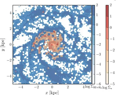
Figure 2.1: Example of one of our maps, made from a Milky Way-mass simulated galaxy atz ≈0 (galaxym12ifrom Hopkins, Kereš, Oñorbe, et al., 2014), with 100 pc pixels. Neutral hydrogen surface density,ΣHI+H2[Mpc

−₂

] and instantaneous gas star formation rate ˙Σ?[M yr−1 kpc−2] are colored in blues and reds, respectively. Spiral arms and increasing density towards the galactic core are clearly visible, and the instantaneous star formation rate is seen to closely trace the densest gas structures.

Krumholz et al. (2009b) attribute the dependence to the gas column needed to

self-shield molecular gas for a given metallicity. As well gas metallicity has been argued

to weakly modulate the specific strength of stellar feedback, as SNe couple slightly

less momentum into their immediate stellar surroundings since more of their energy

is able to radiate away quickly (Cioffi et al., 1988; Martizzi, Faucher-Giguère, et

al., 2015; Richings et al., 2016). Scoville et al. (2016) found evidence of shorter

depletion timescales for molecular gas at higher redshifts for galaxies both on and

above the star formation main sequence, perhaps due to the rapid accretion required

to replenish the gas reservoirs.

Large-volume cosmological simulations often use the KS law as a sub-grid

(33)

of including all of the physics relevant on the scales of star-forming regions, and

their inability to resolve even the most massive giant molecular clouds∼ 106 M

(e.g., Mihos et al., 1994; Springel et al., 2003). Even idealized disk simulations that

have resolution on the order of 100 pc, but are unable to resolve a multiphase ISM,

employ star formation prescriptions that assume low star formation efficiencies a

priorior implement KS laws indirectly (Li et al., 2006; Wada et al., 2007; Schaye

and Dalla Vecchia, 2008; Richings et al., 2016). It has been shown that assuming

a power-law star formation relation on the resolution scale can imprint a power-law

relation of identical slope on the galactic scale (Gnedin, Tasker, et al., 2014),

demon-strating the importance of employing physically motivated sub-grid star formation

prescriptions that produce kpc-scale relations with the ‘correct’ slope if the relevant

physical processes cannot be treated directly. With advances in computing power,

and the ability to execute increasingly complex simulations with more physics at

higher mass resolution, cosmological simulations have only recently been able to

predict the KS relation generically as a result of the physics incorporated in the

simulations at the scales of molecular clouds (e.g., Hopkins et al., 2011; Hopkins,

Cox, et al., 2013; Hopkins, Kereš, Oñorbe, et al., 2014; Agertz and Kravtsov, 2015).

Including realistic feedback physics in simulations that resolve GMC scales is critical

to understanding the KS relation due to the multitude of competing physical effects

spanning a wide range of scales. While some simulations have argued that the KS

relation can be obtained without explicit feedback (e.g., Li et al., 2005; Li et al.,

2006; Wada et al., 2007), these generally depend on either (a) transient and

short-lived initial conditions (e.g. simulations starting from strong initial turbulence

or a smooth disk, where once turbulence decays and fragmentation runs away,

some additional source of “driving” or “GMC disruption” must be invoked), or (b)

suppressing runaway fragmentation numerically (e.g., “by hand” setting very slow

star formation efficiencies at the grid scale, or inserting explicit sub-grid models for

star formation calibrated to the KS relation on GMC or galaxy scales, or adopting

artificial/numerical pressure or temperature floors or fixed gravitational softening in

the gas that prevent densities from increasing arbitrarily). Many of these authors do

acknowledge that feedback is likely necessary to provide either the initial conditions

or grid-scale terms in their simulations, even if not explicitly included (similarly, see

e.g., Robertson et al. 2008; Colin et al. 2010; Kuhlen et al. 2012; Kraljic et al. 2014).

Indeed, a large number of subsequent, higher-resolution numerical experiments (on

scales ranging from kpc-scale “boxes” to cosmological simulations) which run for

(34)

consistently shown that absent feedback, the galaxy-scale KS law has a factor∼100

higher normalization than observed (see e.g., Hopkins et al., 2011; Kim, Kim, et al.,

2011; Ostriker and Shetty, 2011; Shetty and Ostriker, 2012; Kim, Ostriker, and

Kim, 2013; Kim and Ostriker, 2015; Dobbs, 2015; Benincasa et al., 2016; Forbes

et al., 2016; Hu et al., 2017; Iffrig et al., 2017).

In this chapter, we explore the properties and emergence of the KS relation in the

FIRE1(Feedback In Realistic Environments) simulations (Hopkins, Kereš, Oñorbe,

et al., 2014). Specifically, by producing mock observational maps of the spatially

resolved KS law, we investigate the form of the relation when considering several

different tracers of the star formation rate and gas surface densities, and we

charac-terize its dependence on redshift, metallicity, and pixel size. The FIRE simulations

are well suited for understanding the physical drivers of the KS relation as they

sample a variety of galactic environments and a large dynamic range in physical

quantities (chiefly, gas and star formation rate surface densities), and they directly

(albeit approximately) incorporate stellar feedback processes that may be crucial for

the emergence, and maintenance of the KS relation over cosmological timescales.

In the past, they have been used to investigate the effects of various microphysics

prescriptions on galaxy evolution, the formation of giant gas clumps at high redshift,

and the formation of galaxy discs, among other topics (Oklopčić et al., 2017; Ma

et al., 2017; Su et al., 2017).

2.2 Simulations & Analysis Methods

In the present analysis, we investigate the star formation properties of the FIRE

galaxy simulations originally presented in Hopkins, Kereš, Oñorbe, et al. (2014),

Chan et al. (2015), and Feldmann, Hopkins, et al. (2016), which used the Lagrangian

gravity + hydrodynamics solver gizmo (Hopkins, 2013) in its pressure-energy

smoothed particle hydrodynamics (P-SPH) mode (Hopkins, 2013). All of the

simu-lations employ a standard flatΛCDM cosmology withh ≈0.7,ΩM= 1−ΩΛ ≈ 0.27,

andΩb ≈ 0.046. The galaxies in the simulations analyzed in this chapter range in z≈ _{0 halo masses from 9}.₅×₁₀9

to 1.4×1013M, and minimum baryonic particles masses mb of 2.6× 102 to 3.7× 105 M. For all of the simulations, the mass resolution is scaled with the total mass such that the characteristic turbulent Jeans

mass is resolved. As well, the force softening is fully adaptive, scaling with the

1

(35)

particle density and mass as

δh≈₁._{6 pc}

n

cm−3

−1/3 m

103M !1/3

, (2.1)

wherenis the number density of the particles, and mis the particle mass.

Conse-quently, the simulations are able to resolve a multiphase ISM, allowing for

meaning-ful ISM feedback physics. This is crucial because the vast majority of star formation

occurs in the most massive GMCs due to the shape of the GMC mass function

(Williams et al., 1997).

The stellar feedback physics implemented in these simulations include approximate

treatments of multiple channels of stellar feedback: radiation pressure on dust grains,

supernovae (SNe), stellar winds, and photoheating; a detailed description of the

stellar feedback model can be found in Hopkins, Kereš, Oñorbe, et al. (2014). Star

particles in the simulations each represent individual stellar populations, with known

ages, metallicities, and masses. Their spectral energy distributions, supernovae

rates, stellar wind mechanical luminosities, metal yields, etc., are calculated directly

as a function of time using the starburst99 (Leitherer et al., 1999) stellar population

synthesis models, assuming a Kroupa (2002) initial mass function (IMF).

In these simulations, the galaxy- and kpc-scale star formation efficiencies arenotset

‘by hand’. Star formation is restricted to dense, molecular, self-gravitating regions

according to several criteria:

• The gas density must be above a critical threshold, ncrit ∼ 50 cm

−₃

in most

runs (and 5 cm−3in those from Feldmann, Hopkins, et al., 2016).

• The molecular fraction fH2 is calculated as a function of the local column

density and metallicity using the prescription of Krumholz and Gnedin (2011),

and the molecular gas density is used to calculate the instantaneous SFR (see

below).

• Finally, we identify self-gravitating regions using a sink particle criterion

at the resolution scale, specifically requiring α ≡ δv2δh/Gmgas(< δr) < 1

on the smallest resolved scale around each gas particle (δh being the force softening or smoothing length).

Regions that satisfy all of the above criteria are assumed to have an instantaneous

star formation rate of

˙

(36)

i.e. 100 percent efficiency per free-fall time. As a large fraction of the dense

(n > ncrit), molecular (fH2 ∼ 1) gas is not gravitationally bound (α > 1) at any given time, theglobal star formation efficiency is less than 100 percent ( < 1) despite the assumedlocal, instantaneousstar formation efficiency per free-fall time

being 100 percent. We will show below that the KS relation, with its much lower

global, time-averaged star formation efficiency ( . 0.1), emerges as a result of

stellar feedback preventing dense gas from quickly becoming self-bound, forming

stars, and disrupting gravitationally bound star-forming clumps on a timescale less

than the local free-fall time. We stress here that the emergent KS relation is nota

consequence of the star formation prescription employed in the simulations.

In Appendix 2.5 we demonstrate this explicitly. We ran several tests restarting

one of the standard FIRE simulations with varying physics and star formation

prescriptions. For any reasonable set of physics, only variation in the strength of the

feedback affected the galactic star formation rates, because the simulated galaxies

self-regulate their star formation rates via feedback. A number of independent

studies have also shown that once feedback is treated explicitly, the predicted KS

law becomes independent of the resolution-scale star formation criterion (Saitoh

et al., 2008; Federrath et al., 2012; Hopkins et al., 2012a; Hopkins, Kereš, Murray,

et al., 2013; Hopkins, Cox, et al., 2013; Hopkins, Narayanan, et al., 2013; Hopkins,

Torrey, et al., 2016; Agertz, Kravtsov, et al., 2013).

To quantify the spatially resolved KS relation in the simulations, we analyze data

from snapshots spanning redshifts z = 0−6. The standard FIRE snapshots from

Hopkins, Kereš, Oñorbe, et al. 2014 and the dwarf runs in Chan et al. (2015) are

roughly equipartitioned among redshift bins z ∼ 3−6, 2.5−1.5, 1.5−0.5, and

< 0.5, whereas the snapshots of halos from Feldmann, Hopkins, et al. (2016) have

redshifts evenly spaced between 2 < z < 6 (these were run to only z ∼ 2). To compare the snapshots with observational constraints of the KS relation, we made

star formation rate and gas surface density maps of each snapshot’s central galaxy.

We summed the angular momentum vectors of the star particles in the main halo

of each snapshot to determine the galaxy rotation axis and projected along this axis

to generate face-on galaxy maps. The projected maps were then binned into square

pixels of varying size, ranging from 100 pc to 5 kpc on a side. Only particles within

20 kpc above or below the galaxy along the line of sight were included in the maps

(this captures all of the star-forming gas, but excludes distant galaxies projected by

(37)

resulting maps can be found in Figure 2.1, which shows maps of the neutral gas

surface density and the instantaneous star formation rate surface density in them12i

simulation from Hopkins, Kereš, Oñorbe, et al. (2014), at redshift z ≈ 0 with 100

pc pixels.

Using the star particle ages, we calculated star formation rates averaged over the

previous 10 and 100 Myr, correcting for mass loss from stellar winds and other

evolutionary effects as predicted by starburst99 (Leitherer et al., 1999). We

also considered the instantaneous star formation rate of the gas particles (defined

above). A time-averaging interval of 10 Myr was chosen because this approximately

corresponds to the timescale traced by recombination lines such as Hα, whereas UV and FIR emission traces star formation over roughly the past 100 Myr (e.g.,

Kennicutt and Evans, 2012).2 The instantaneous star formation rate of the gas

particles covers a larger range of star formation rates because it is not constrained

at the low end directly by the mass resolution of our simulations; it is a continuous

quantity intrinsic to the gas particles themselves, which is sampled at each time-step

to determine if the gas particles form stars. This quantity best demonstrates the direct

consequences of feedback on the gas in situ by locally tracing the star formation

rate, whereas the other two SFR tracers are more analogous to observables.

The gas surface density tracers were also chosen on the basis of observable

ana-logues, including all gas, neutral hydrogen gas (total HI + H2column, accounting

for metallicity and He corrected), and “Cold & Dense” gas which we specifically

define here and throughout this chapter as gas withT < 300 K and nH > 10 cm

−₃

.

These roughly correspond to the total gas (including the ionized component), atomic

+ molecular gas (HI+H2), and cold molecular gas reservoirs observed in

galax-ies. We have opted to use the aforementioned approximation for the molecular gas

component rather than reconstruct the fH2 predicted by the Krumholz and Gnedin

(2011) model (which is not output in the snapshots) as the fH2 model assumes a

simplified geometry at the resolution scale, that can get the local optical depth quite

wrong3. We explore the differences between the Cold & Dense gas tracer and the

2

Directly computing SFR indicators from the simulations (e.g., Hayward, Lanz, et al., 2014; Sparre et al., 2015) rather than computing the SFR averaged over the past 10 or 100 Myr would pro