Enhanced "vector-cross-product" direction-finding using a constrained sparse triangular-array

R E S E A R C H

Open Access

Enhanced

“

vector-cross-product

”

direction-finding

using a constrained sparse triangular-array

Feng Luo

and Xin Yuan

Abstract

A new configuration of sparse array is proposed in this article to estimate the direction-of-arrivals (DOAs) and polarizations of multiple sources. This constrained sparse array is composed of a dipole-triad, a loop-triad, and a single antenna, which can be a dipole, a loop, or a scalar-sensor. These three units comprise a triangular geometry in the space. This geometry creatively synergizes the conventional interferometry method based on the spatial phase-delay across displaced antennas, and the“vector-cross-product”based on Poynting-vector estimator to enhance the DOA estimation accuracy. The investigated algorithm based on this configuration adopts the“ vector-cross-product” DOA estimator to provide thecoarseestimate and then derives thefineestimate by extracting the inter-sensor phase factors in the sparse array. Following this, the disambiguation approach is adapted to derive the unambiguous estimate, and this estimate is also fine in estimation resolution. The proposed configuration can extend the array aperture and also reduce the mutual coupling. The significant performance of the proposed sparse array composition is demonstrated by Monte Carlo simulations when the inter-sensor spacing far exceeds a half-wavelength.

Keywords:antenna array mutual coupling, antenna arrays, aperture antennas, array signal processing, direction of arrival estimation, polarization.

1. Introduction

The basic principle of the“vector-cross-product” direc-tion-finding is to extract the relations between the

elec-tric-field e and the magnetic-field h of an

electromagnetic wave. The vector-cross-product betweeneand h, the Poynting-vectoru, will provide the direction-cosines of the incident source. It follows that the direction-of-arrival (DOA) of the source can be estimated.

This “vector-cross-product” direction-finding algo-rithm was proposed by Nehorai and Paldi based on the component electromagnetic vector-sensor. A six-component electromagnetic vector-sensor consists of three orthogonal dipoles and three orthogonal loops. These dipoles and loops are collocated at a point geo-metry in space, in order to measure the electric-field and magnetic-field of the incident signal, respectively. In a multiple source scenario withKincident sources, the

responses of thekth sourceakcan be represented by the 3 × 1 electric-field vector ek and the 3 × 1 magnetic-field vectorhk[1,2]:

akdef

ek

hk

def

⎡ ⎢ ⎢ ⎢ ⎢ ⎢ ⎢ ⎣

ex,k ey,k ez,k hx,k hy,k hz,k

⎤ ⎥ ⎥ ⎥ ⎥ ⎥ ⎥ ⎦

def

⎡ ⎢ ⎢ ⎢ ⎢ ⎢ ⎢ ⎣

cosθ1,ksinθ2,ksinθ3,kejθ4,k−_sinθ

1,kcosθ3,k

sinθ1,ksinθ2,ksinθ3,kejθ4,k_{+ cos}θ

1,kcosθ3,k

−cosθ2,ksinθ3,kejθ4,k

−sinθ1,ksinθ3,kejθ4,k−_cosθ

1,ksinθ2,kcosθ3,k

cosθ1,ksinθ3,kejθ4,k−_sinθ

1,ksinθ2,kcosθ3,k

cosθ2,kcosθ3,k

⎤ ⎥ ⎥ ⎥ ⎥ ⎥ ⎥ ⎦

, (1)

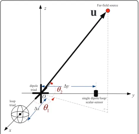
where {θ1,kÎ [0, 2π),θ2, kÎ [-π/2,π/2]} are the azi-muth-angle and elevation-angle of the source (please refer to Figure 1), respectively, and {θ3,kÎ[0, π/2],θ4,k

Î [-π, π)} denote the auxiliary polarization angle and polarization phase difference of the incident signal, respectively (equating to {g,h} in [3]). The unique array-manifold in (1) has been exploited extensively by various eigenstructure-based direction-finding frameworks [2-43].

Based on (1), the Poynting-vectoruk of the kth inci-dent source can be obtained by [1]:

* Correspondence: [email protected]

2

Department of Electrical and Computer Engineering, Duke University, Durham, NC 27708, USA

Full list of author information is available at the end of the article

uk=

ek×h∗k ——ek×h∗k||

=

⎡

⎣coscosθθ2,2,kkcossinθθ1,1,kk sinθ2,k

⎤ ⎦def

⎡ ⎣uuxy,,kk

uz,k

⎤ ⎦,(2)

where * denotes complex conjugation, × symbolizes the vector cross-product operator, || · || represents the Frobenius norm of the element inside || ||, and {ux, k, uy, k, uz, k} are the direction-cosines of thekth source align tox-axis, y-axis,z-axis, respectively. From thisuk, the DOA (θ1,k,θ2, k) of thekth source can be derived uniquely in the three-dimensional space. Equation (2) also indicates that the azimuth-angle and elevation-angle of each source can be automatically paired with-out post-processing [2].

Wong et al. advanced the “vector-cross-product”

direction-finding algorithm by investigating some novel capabilities of the electromagnetic vector-sensor (array), for example, sparse array with six-component electro-magnetic vector-sensor [10], DOA estimation without the priori known sensors’ locations [9],“self-initiating

MUSIC” [12] and blind geolocation, beamforming for

frequency-hopping sources of unknown and arbitrary hop-sequences [13].

One remarkable innovation to adapt the“ vector-cross-product” direction-finding algorithm is the “Displaced Dipole-Triad-Plus-Loop-Triad Pair” proposed in [44]. The“vector-cross-product”direction-finding algorithm is found still applicable when the dipole-triad and loop-triad are spatially spread in the space. Reference [44] adopted the “vector-cross-product”to do the direction-finding with this “Displaced Dipole-Triad-Plus-Loop-Triad Pair”, and also compared the Cramér-Rao bounds

(CRBs) of this configuration with that of the collocated electromagnetic vector-sensor to show that the displaced pair can offer a lower CRBs. The advantages of the“

Dis-placed Dipole-Triad-Plus-Loop-Triad Pair” compared

with the collocated electromagnetic vector-sensor are significant:

(1) The collocated antennas are reduced from six to three, and thus the mutual coupling across the com-posed antennas are reduced greatly.

(2) Since the dipole-triad and the loop-triad are spa-tially spread and there is no constraint of their relative locations, the spatially array aperture is extended and so the estimation accuracy for DOA can be improved distinctly.

Wong [44] proposed this configuration and presented an example with CRBs to show that this configuration can improve the direction finding accuracy. However, the algorithm used in [44] was only the“ vector-cross-product”result, which is the same as thecollocated elec-tromagnetic vector-sensor. Therefore, the approach uti-lized in [44] can not investigate the advantage (2) described above. Based on this, the present article will propose a new configuration based on the “Displaced Dipole-Triad-Plus-Loop-Triad Pair” in [44], and will investigate an enhanced algorithm to extract the aper-ture extension property of the new configuration. This enhanced algorithm will then improve the direction-finding estimation accuracy by extracting the inter-sen-sor phase factors across the seninter-sen-sors, which were ignored in [44].

For the 2D elevation-azimuth angle estimation, two phase-factors are necessary. Therefore, a constrained sparse triangular-array is proposed in this article. The triangular-array consists of a dipole-triad, a loop-triad, and a single dipole/loop/scalar-sensor. It is worth noting that an additional antenna is employed in this triangu-lar-array, which is used to increase the array-aperture. In the derived DOA estimation algorithm, it will provide another inter-sensor phase factor, which is used to derive the fine estimate of one direction-cosine. The enhanced direction-cosines’estimates will improve the direction finding estimation accuracy. In addition, this antenna can be a dipole, a loop, or a scalar-sensor with-out polarization information. The single dipole or loop can be oriented along any one of the three Cartesian coordinate axes. The proposed array geometry is a sparse array with inter-sensor spacings far larger than a half-wavelength. Similar sparse vector-sensor arrays have been investigated in [10,11,36,45].

Another remarkable innovation to adapt the “ vector-cross-product” direction-finding algorithm is the“ non-collocating electromagnetic vector-sensor”proposed in [45]. The six antennas composed of the electromagnetic vector-sensor are spatially spread in the space with 2

[

\ ]

GLSROH WULDG

VLQJOHGLSROHORRS VFDODUVHQVRU ORRS

WULDG

[

Δ

\

Δ

)DUILHOGVRXUFH

X

θ

θ

some constrains. Then the “vector-cross-product” direc-tion-finding algorithm can still be used. Furthermore, the mutual coupling is reduced and the angular resolu-tion is enhanced. In addiresolu-tion, it is also shown in [45] that the“uni-vector-sensor ESPRIT” algorithm proposed in [2] can still be utilized in the non-collocating electro-magnetic vector for direction finding. This“ uni-vector-sensor ESPRIT”algorithm will thus be used in the pre-sent article in the following derivation and also in the simulation. However, the algorithm investigated in [45] can only offer one fine estimate of the direction-cosine, and this is not sufficient for the 2D direction finding. Based on this reason, the present article proposes a new configuration with seven sensors to form a triangular array, in order to increase the array aperture and then to improve the two dimensional DOA estimation accu-racy. It is worth noting that the dipole-triad and loop-triad can be non-collocating but need to satisfy the con-ditions proposed in [45]. In order to simplify the exposi-tion, the following derivation will be based on the collocated case.

The dipole-triad and loop-triad have also been exten-sively investigated in other literature. The anti-jamming performance of the dipole-triad (a.k.a. tripole) has been investigated by Comption Jr. [46,47]. The dipole-triad (array) was used for direction finding in [48-52]. The performance of a dipole-triad array for 1D direction finding and polarization estimation has been evaluated in [48] through the CRBs derivation, and it showed that the quality of the DOA estimate depends strongly on the polarization state. Zhang [49] investigated an ESPRIT based algorithm for direction finding and polar-ization estimation for uniform circular dipole-triad array, and Zainud-Deen et al. [50] adopted the radial basis function neural network to the uniform circular dipole-triad array (and also cross-dipole array) for direc-tion finding and polarizadirec-tion estimadirec-tion. Daldorff et al. [53] combined unitary matrix pencil method and a least squares solver to do the direction finding with a single dipole-triad. The linear dependence and uniqueness of dipole-triad (dipole-triad array) was developed in [54-57]. AnH∞ approach was proposed in [58] to track polarized cochannel sources with dipole-triad array, and a new quasi-cross-product algorithm was proposed in [59] for tracking the direction of a moving and nonli-nearly polarized electromagnetic source using a dipole-triad. Zhang and Xu [60] explored blind beam-forming of the dipole-triad array and the parallel factor model was adopted. Ravinder and Pandharipande [61,62] showed that a dipole-triad could minimize bit error rate better through polarization diversity when the desired user and other interfering users arrived from the same direction or were very close to the desired user direction but with different polarization states. Theoretical

performance bounds for direction finding using the dipole/loop triad were derived in [63].

The remainder of this article is organized as follows. The geometry of the sparse triangular-array is provided

in Section 2. The enhanced “vector-cross-product”

direction-finding algorithm based on the proposed con-figuration is derived in Section 3. Section 4 presents the simulation results of the enhanced algorithm, and Sec-tion 5 concludes the whole article.

2. Spatial geometry of the sparse array used in this work

Wong [44] investigated the “vector-cross product” for direction finding with spatially spaced dipole and loop triad but ignored the effect of spatial phase-factor, which can improve the accuracy of direction finding. In order to get thefinerestimate for the DOA, at least two finer direction-cosines’ estimates should be obtained.

The dipole-loop triad pair can present three coarse

direction-cosines’ estimates from the“vector-cross pro-duct” result and one finer direction-cosine’s estimate from the inter-triad spacing phase. Thus, another antenna is employed to provide the other finer direc-tion-cosine’s estimates from the inter-sensor spacing phase factor and at the same time to increase the array aperture. Figure 1 depicts the array geometry used in this work.

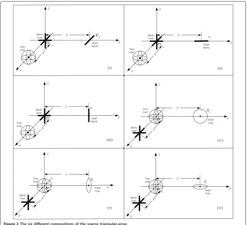
Figure 2 illustrates the six different sparse array com-positions, and each composition is made up of seven dipoles/loops. The seven dipoles/loops are categorized into three different units: (1) one collocated dipole-triad, (2) one collocated loop-triad, and (3) one single dipole/ loop of various orientations.

The array-manifold of the compositions in Figure 2 can be classified into two groups:

(A) Cases (i)-(iii), the dipole-triad is located at the ori-gin of the Cartesian coordinate system, the loop-triad is located at (Δx, 0, 0) on thex-axis, and the single dipole is located on they-axis at (0,Δy, 0). The array-manifold can be shown as:

a=

⎡ ⎣q1eh

q2b

⎤ ⎦=

⎡ ⎢ ⎢ ⎣

e

e−j2π xλuxh e−j2π

yuy

λ b

⎤ ⎥ ⎥

⎦ (3)

where

q1defe −j2πxux

λ ,q2defe −j2πyuy

λ , and b is one of

{ex, ey, ez} corresponding to the different cases.

a=

⎡ ⎣qh1e

q2b

⎤

⎦ (4)

wherebis one of {hx, hy, hz} corresponding to the dif-ferent cases.

Remarks:

• The single dipole/loop can be replaced by one

dipole/loop triad and thus the compositions will have three dipole/loop triads: (a) one dipole-triad and two loop-triads, (b) one loop-triad and two dipole-triads. Under those configurations, the“vector-cross-product” can be obtained three times and hence the average value can be used. Also the two fine estimates of

direction-cosines are both obtained from the inter-triad phase fac-tors of the“vector-cross-product”results.

• The single dipole/loop in Figure 2 can be located at an arbitrary position (x2, y2), but not collinear with the

dipole-triad and loop-triad.

• The relative locations of dipole-triad, loop-triad and the single dipole/loop can be changed, Figure 2 just pre-sents six examples.

•The single dipole/loop in Figure 2 can be replaced by a scalar-sensor, and this scalar-sensor will not include the polarization information of the incident source. In this case, thebin (3)-(4) will be replaced by 1.

• The proposed sparse-array is different from the

sparse-array in [10,11], where the array is composed of \

[

[

[

[ 2

[

\ ]

GLSROH WULDG

VLQJOH GLSROH ORRS

WULDG

[

H

2

[

\ ]

GLSROH WULDG

VLQJOH GLSROH ORRS

WULDG

\

H

2

[

\ ]

GLSROH WULDG

VLQJOH GLSROH ORRS

WULDG

]

H

2

[

\ ]

GLSROH WULDG

VLQJOH ORRS ORRS

WULDG K[

2

[

\ ]

GLSROH WULDG

VLQJOH ORRS ORRS

WULDG K\

2

[

\ ]

GLSROH WULDG

VLQJOH ORRS ORRS

WULDG K]

L LL

LLL LY

Y YL

[

[

\ \

\ \

\

six-component electromagnetic vector-sensors. The pro-posed array pioneers the geometry with three different sensors and it has two advantages compared with the sparse array in [10,11]: (a) The triad only has three col-located antennas, thus the new array configuration can reduce the mutual coupling; (b) The new array config-uration can diminish the hardware cost as only the triad and single dipole/loop is used. Furthermore, the single dipole/loop can be replaced by the simple scalar-sensor.

As the following analysis is similar for all the six cases, case (i) will be taken as an example to derive the enhanced “vector-cross product” algorithm for direc-tion-finding. Please note that the classical far field and narrow-band assumption is made throughout the article.

3. The enhanced“vector-cross product” algorithm for direction finding

From various eigenstructure-based parameter estimation algorithms cited in Section 1, the steering vector of the kth incident source can be obtained, within an unknown complex numberc[44,45]. That is:

ˆ

ak

def

≈ cak. (5)

All the following derivation for the enhanced “ vector-cross product”algorithm will be based on (5). The deri-vation steps are similar to the algorithm proposed in [45]. First, the course but unambiguous estimates of direction-cosines are derived from the“ vector-cross-pro-duct” result. Then, the fine but cyclically ambiguous estimates of direction-cosines are obtained from the inter-sensor phase factors. Finally, the coarse estimates of direction-cosines are used to disambiguate the fine but cyclically ambiguous estimates to derive both fine and unambiguous estimates of direction-cosines.

3.1. Get the coarse but unambiguous estimates of direction-cosines from the“vector-cross-product”result From (5), for case (i) in Figure 2, in the multiple source scenario withKincident sources,

ˆ

ak=c

⎡ ⎣q1,ekkhk

q2,kex,k

⎤

⎦, (6)

and from the vector-cross product [44],

˜

uk=

(ceˆk)×(cq1,khˆk)

∗

||(ceˆk)×(cq1,khˆk)

∗ || =q

∗ 1,k

⎡ ⎣uuxy,,kk

uz,k

⎤

⎦. (7)

Note that ũkis different from the Poyting vector uk (see Figure 1), but it can be seen as an estimate of uk,

˜

uk=q∗1,kuk. It follows that uk can be estimated from thisũk. Separately consider the following two cases:

(1) Ifθ2,kÎ[0,π/2], which meansuz, k≥0, then:

ˆ

uk=u˜ke−j [uˆk]3=

⎡ ⎣uˆ

coarse

x,k

ˆ ucoarse_y,k

ˆ uz,k

⎤

⎦, (8)

where [·]iis theith element of the vector in [ ], and∠ denotes the complex angle of the following complex number.

(2) Ifθ2,kÎ[-π/2, 0), which isuz, k≤0, then:

ˆ

uk=− ˜uke−j [u˜k]3 =

⎡ ⎣uˆ

coarse

x,k

ˆ ucoarse

y,k

ˆ uz,k

⎤

⎦. (9)

It follows that:

ˆ ucoarse

x,k = [uˆk]1, (10)

ˆ

ucoarse_y,k = [uˆk]2. (11)

3.2. Obtain the fine but cyclically ambiguous estimates of direction-cosines

The inter-sensor phase-factors {q1,q2} can offer the fine

estimates for the direction-cosines. However, they will suffer the cyclically ambiguous because of the periodicity of the phase. From the vector-cross product result in (7),

(1) ifθ2,kÎ[0,π/2],

ˆ

ufine_x,k = λk

2π

1

x

[u˜k]3; (12)

(2) ifθ2,kÎ[-π/2, 0],

ˆ

ufine_x,k = λk

2π

1

x

( [u˜k]3+π). (13)

From (6), uˆfine_y,k can be obtained by:

ˆ

ufine_y,k = λk

2π

1

y

[aˆk]1

[aˆk]7

. (14)

Remarks:

• The cases (1) and (2) in (8)-(9) and (12)-(13) are based on the condition whetheruz, kis positive or nega-tive, which leads to that the validity region of direction-finding is the upper hemisphere or lower hemisphere in the polar coordinate system. Therefore, the ∠[ũk]3 is

used in (12) and (13).

If the condition changes to be based on the positive or negative of ux, k, the validity region of direction-finding will be the front hemisphere or back hemisphere in the polar coordinate system. In this case, the ∠[ũk]1 will be

If the condition changes to be based on the positive or negative ofuy, k, the validity region of direction-finding will be the left hemisphere or right hemisphere in the polar coordinate system. In this case, the ∠[ũk]2 will be

used in Section 2.

• uˆcoarse

x,k , uˆ

coarse

y,k , uˆfinex,k are the same for all the six cases

in Figure 2, but the uˆfine_y,k varies for different cases based on the array-manifold. For cases (i)-(vi) in Figure 2, uˆfine

y,k

can be estimated from uˆfine_y,k = ₂λ_π1

y

[aˆk]i [aˆk]7

, ∀i = 1, 2,

..., 6, corresponding to each case.

• If the scalar-sensor is used to replace the single dipole/loop, since the response of hzis a positive real

number, uˆfine_y,k can be estimated from

ˆ ufine_y,k = λk

2π1y

[aˆk]6

[aˆk]7

.

•The single dipole/loop/scalar-sensor in Figure 1 can be located at an arbitrary position (x2,y2), but not

colli-near with the dipole-triad and loop-triad. Then the

array-manifold will be

ak=

⎡ ⎢

⎣ek,q1,khk,e

−j2π

λk

(x2ux,k+y2uy,k) bk

⎤ ⎥ ⎦

T

. In this case, after

the ûx, k is derived, uˆfiney,k can be obtained through

λk 2πy12

[aˆk]i [aˆk]7

− x2

y2uˆx,k

, where i = 1, 2, ..., 6

corre-sponds to the number of element in the array-manifold. The disadvantage of this arbitrary location configuration is that it will increase the computation workload of the estimation algorithm.

3.3. Disambiguate the fine estimates by coarse estimates of direction-cosines

In order to get the fine and unambiguous estimates of the direction-cosines, the coarse estimates obtained in Section 1 will be used as the reference to disambiguate the fine estimates derived in Section 2. This disambigua-tion approach has been derived by Zoltowski and Wong [10], and has also been used in the other literature, i.e. [11,45]. The main essence is summarized as follows [45]. Using {ûx, k, ûy, k} to denote the fine and unambiguous estimates of the direction-cosines, there exist two inte-gers {mo_x,k, mo_y,k} leading to [45]:

ˆ

ux,k=uˆxfine,k +mox,k

λk

x

, (15)

ˆ

uy,k=uˆfiney,k +m

o

y,k

λk

y

. (16)

{mo

x,k, moy,k} can be derived by:

mo_x,k = arg minmx,k

uˆcoarse_x,k − ˆufine_x,k −mxλk

x

,

mo_y,k =arg minmy,k

uˆcoarse_y,k − ˆufine_y,k −myλk

y

,

for

mx,k ∈

x λk

−1− ˆucoarse_x,k ,

x λk

1− ˆucoarse_x,k ,

my,k ∈

y λk

−1− ˆucoarsey,k

, y λk

1− ˆucoarsey,k

,

where⌈a⌉denotes the smallest integer not less than a, and ⌊a⌋refers to the largest integer not exceedinga.

However, in case that Δx ≤ lk, Δy ≤ lk, the spatial aperture is not much extended. We can set uˆx,k=uˆcoarse_x,k ,

ˆ

uy,k=uˆcoarsey,k , directly.a

Lastly, after the unique {ûx, k,ûy, k} has been obtained, the DOA ofkth incident source {θ1,k,θ2,k} can be esti-mated by [2,45]:

ˆ

θ1,k= arctan

_ˆ uy,k

ˆ ux,k

, (17)

ˆ

θ2,k= arcsin

ˆ u2_y,k+uˆ2_x,k

. (18)

The polarization parameters can be estimated byâk:

ˆ

θ3,k= arctan

[aˆk]3

[aˆk]6

, (19)

ˆ

θ4,k=

⎧ ⎨ ⎩

[aˆk]3

ˆ

q∗1,k[ˆak]6

−π, for case (i)–(iii) in Figure 2;

ˆq∗1,k[ˆak]3 [aˆk]6

−π, for case (iv)–(vi) in Figure 2. (20)

where ˆ q1,k=e

−j2π

λk

xuˆx,k.

4. Monte Carlo simulation for the algorithm obtained in Section 3

The proposed algorithm’s direction-finding efficacy and extended-aperture capability are demonstrated by Monte Carlo simulations and the accuracy is compared with the conventional “vector-cross product” (CVC) algorithm in [44]. In the plotted figures, the curves with the proposed algorithm are labeled with EVC and the curves with conventional “vector-cross product”

algo-rithm are labeled with CVC. The “uni-vector-sensor

steering vectors of the incident sources (to derive Equa-tion (5)) in the following simulaEqua-tions and thus the sources are modeled as uncorrelated pure tones with different frequencies. The estimates use 400 temporal snapshots and 500 independent runs. The root mean square error (RMSE) is utilized as the performance

mea-sure. The RMSE for the direction-cosine of the kth

source is defined as

RMSE =

1

500

500

i=1

ˆ ui

x,k−ux,k

2

+uˆi y,k−uy,k

2

,

where {ˆui_x,k,uˆi_y,k} are the estimate of direction-cosines atith run.

4.1. Compare the proposed algorithm (EVC) with the conventional“vector-cross product”algorithm (CVC) and CRBs

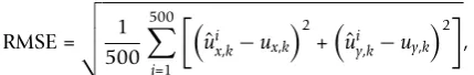
Figure 3a shows a two-source scenario results, whereas Figure 3b shows a three-source scenario results. Both the estimation bias and RMSE of the direction-cosine are plotted in Figure 3. Figure 3 clearly demonstrates that the performance of proposed algorithm (EVC) is better than that of the conventional “vector-cross

pro-duct” algorithm (CVC), especially when SNR ≥ 5 dB.

The RMSE for direction-cosine with the proposed algo-rithm is ten times lower than the RMSE with the CVC, and they are very close to the CRBs.bFigure 4 plots the standard deviations of estimates for the DOA (θ1,k,θ2,

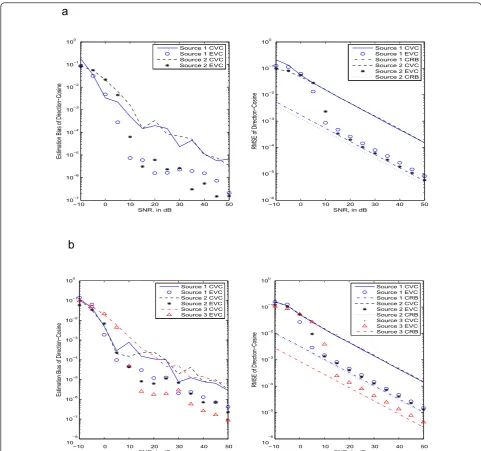
k) versus SNR for each source in a two-source scenario as in Figure 3a. It can be seen that when SNR≥ 5 dB, the standard deviations of the (θ1,k, θ2,k) with the pro-posed algorithm are about 30 times lower than their counterparts with the CVC, and they are very close to the CRBs. Figures 3 and 4 clearly verify the performance of the proposed array-geometry and also verify the effi-cacy of the proposed algorithm.

4.2. The aperture extension of the proposed configuration

It is well known that the larger is the array’s spatial aperture, the finer would be the resolution of the arrival angle estimates, so it is of interest to investigate the per-formance of the proposed sparse array when the spatial aperture becomes larger.

Figure 5a shows a two-source scenario, whereas Figure 5b shows a three-source scenario with the same setting as in Figure 3 at SNR = 30 dB, by plotting the RMSE of the direction-cosines estimates versus inter-sensor spa-cing _λ, wherelis the minimum wavelength of the inci-dent sources. Figure 5 clearly shows that the RMSE of the direction-cosines estimates with the proposed

algorithm decrease with the increase of the spatial aper-ture and they are very close to the CRBs. This proposed configuration and the enhanced algorithm lead to orders-of-magnitude improvement in estimation accu-racy. However, the RMSE of the direction-cosines esti-mates with the conventional “vector-cross product” algorithm remain the same with the increase of the spa-tial aperture. It can also be observed that when_{λ ≤}2, the performance of the two algorithm is nearly the same and it is better to use the conventional “vector-cross product”algorithm since it needs less manipulation. It is worth noting that a breakdown phenomenon initiates in Figure 5 at an inter-sensor spacing of about Δ= 100l (200 half wavelengths). This is because the coarse mates of direction-cosines begin to misidentify the esti-mation grid. For further investigation of this breakdown phenomenon, please refer to [10].

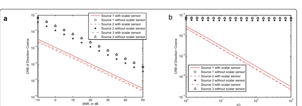
In order to investigate the increased aperture induced by the additional scalar sensor, Figure 6 plots the CRBs of the direction-cosines in a three sources scenario. Both the CRBs with and without the scalar sensor are plotted.“With the scalar sensor” means that the array geometry in Figure 1 is used with the additional antenna as a scalar sensor. “Without the scalar sensor” means that only the dipole-triad and the loop-triad are Figure 1 is used. It can be found from Figure 6a that at each point of SNR, the CRBs with the scalar sensor is about 20 times smaller than the CRBs without the scalar sen-sor. Thus, the additional scalar sensor increases the array-aperture significantly and following this, the DOA estimation accuracy is improved. When SNR = 30 dB, Figure 6b plots the CRBs versus the inter-sensor spacing Δ/l. It can also be found that when the inter-sensor spacings increase, the falling-rate of CRBs for the pro-posed array geometry with the scalar sensor is much faster than its counterpart for the array without the sca-lar sensor. Again, the additional scasca-lar sensor increases the array aperture and so enhances the angular resolution.

5. Conclusion

by only one dipole-triad, one loop-triad and one single dipole/loop/scalar-sensor. Therefore, the mutual cou-pling across the sensors is reduced and additionally the hardware cost is decreased.

Endnotes

a

The proposed array-geometry has an improved iden-tifiability compared with the electromagnetic

vector-sensors in [2,44,45] since an additional antenna is employed. The basic principle of the subspace-based parameter estimation algorithms, such as ESPRIT, is to separate the signal and the noise, into the different sub-spaces (i.e. the signal subspace and the noise subspace), which are derived from the data covariance matrix [64]. It follows that the number of incident sources should be less than the maximal rank of the data covariance

a

b

−10 0 10 20 30 40 50 10−7

10−6

10−5

10−4

10−3

10−2

10−1 100

SNR, in dB

Estimation Bias of Direction

−

Cosine

Source 1 CVC Source 1 EVC Source 2 CVC Source 2 EVC

−10 0 10 20 30 40 50 10−6

10−5 10−4

10−3

10−2

10−1

100

SNR, in dB

RMSE of Direction

−

Cosine

Source 1 CVC Source 1 EVC Source 1 CRB Source 2 CVC Source 2 EVC Source 2 CRB

−10 0 10 20 30 40 50 10

−8

10−7

10−6

10−5

10−4 10−3

10−2

10−1 100

SNR, in dB

Estimation Bias of Direction

−

Cosine

Source 1 CVC Source 1 EVC Source 2 CVC Source 2 EVC Source 3 CVC Source 3 EVC

−10 0 10 20 30 40 50 10

−6

10−5 10−4

10−3 10−2

10−1

100

SNR, in dB

RMSE of Direction

−

Cosine

Source 1 CVC Source 1 EVC Source 1 CRB Source 2 CVC Source 2 EVC Source 2 CRB Source 3 CVC Source 3 EVC Source 3 CRB

Figure 3The estimation bias and RMSE of the direction-cosines estimates versus signal-to-noise ratio (SNR).(a)fortwoincident sources,

at digital frequencies f₁= 0.2565 andf₂= 0.3665, respectively with (θ1,1,θ2,1,θ3,1,θ4,1) = (30°, 60°, 45°, 54°) and (θ1,2,θ2,2,θ3,2,θ4,2) = (20°,

80°, 63°, -90°) CVC denotes the conventional vector-cross productalgorithm while EVC symbolizes the proposed algorithm. The case (i) in Figure

2 is used. The inter-sensor spacingΔx=Δy= 10l,l= min{l1,l2};(b)forthreeincident sources, at digital frequencies f₁ = 0.1055,

f₃ = 0.4315, f₃ = 0.4315, respectively with (θ1,1,θ2,1,θ3,1,θ4,1) = (40°, 20°, 45°, 90°), (θ1,2,θ2,2,θ3,2,θ4,2) = (30°, 60°, 63°, 54°) and (θ1,3,θ2,3,

b

a

−10 0 10 20 30 40 50 10−4

10−3 10−2

10−1

100 101

102

SNR, in dB

Standard Deviation of

θ 1

(degrees)

Source 1 CVC Source 1 EVC Source 1 CRB Source 2 CVC Source 2 EVC Source 2 CRB

−10 0 10 20 30 40 50 10−4

10−3 10−2

10−1

100 101

102

SNR, in dB

Standard Deviation of

θ 2

(degrees)

Source 1 CVC Source 1 EVC Source 1 CRB Source 2 CVC Source 2 EVC Source 2 CRB

Figure 4The standard deviations of the estimates for (θ1,k,θ2,k) versus SNR, in a two-source scenario with the same setting as in

Figure 3a.

b

a

100 101 102 103

10−7

10−6

10−5

10−4

10−3

10−2

Δ/λ

RMSE of Direction

−

Cosine

Source 1 CVC Source 1 EVC Source 1 CRB Source 2 CVC Source 2 EVC Source 2 CRB

100 ₁₀1 ₁₀2 ₁₀3

10−7

10−6 10−5

10−4 10−3

10−2

Δ/λ

RMSE of Direction

−

Cosine

Source 1 CVC Source 1 EVC Source 1 CRB Source 2 CVC Source 2 EVC Source 2 CRB Source 3 CVC Source 3 EVC Source 3 CRB

Figure 5The RMSE of the direction-cosines estimates versus inter-sensor spacingΔ/l.(a)fortwoincident sources; same setting as in

Figure 3a at SNR = 30dB.l= min{l1,l2},Δ=Δx=Δy;(b)forthreeincident sources; same setting as in Figure 3b at SNR = 30dB.l= min{l1,

l2,l3},Δ=Δx=Δy.

b

a

−10 0 10 20 30 40 50 10−6

10−5 10−4 10−3

10−2

10−1

SNR, in dB

CRB of Direction

−

Cosine

Source 1 with scalar sensor Source 1 without scalar sensor Source 2 with scalar sensor Source 2 without scalar sensor Source 3 with scalar sensor Source 3 without scalar sensor

100 101 102 103

10−7 10−6 10−5

10−4

10−3

Δ/λ

CRB of Direction

−

Cosine

Source 1 with scalar sensor Source 1 without scalar sensor Source 2 with scalar sensor Source 2 without scalar sensor Source 3 with scalar sensor Source 3 without scalar sensor

Figure 6Aperture extension effect of the proposed array configuration.(a)The CRBs of the direction-cosines versus SNR, forthreeincident

sources; same setting as in Figure 3b. Both the CRBs with and without the scalar sensor are plotted.(b)The CRBs of the direction-cosines versus

matrix. When the “uni-vector-sensor” algorithm [2] is used in the present array-geometry, the maximal rank of the data covariance matrix equals 7. On the other hand, For the collocated electromagnetic vector-sensor [2], non-collocating electromagnetic vector-sensor [45], or the “Displaced Dipole-Triad-Plus-Loop-Triad Pair”[44], it equals 6. Therefore, when the “uni-vector-sensor” algorithm [2] is used with distinguishable DOAs and polarizations, the resolvable monochromatic sources number should be less than seven, which is one more that the electromagnetic vector-sensors in [2,44,45]. Thus, the additional antenna improves the identifiability compared with the electromagnetic vector-sensor. For more investigations of this identifiability issue with the electromagnetic vector-sensor, please refer to [65-67].

b

The CRBs plotted in the figures in this section is com-puted by the same method as in [45], with the same sig-nal model and noise model. Since the closed-form results are too long to be listed here, we just plot the corresponding curves in the graphs.

Author details

1_{National Lab of Radar Signal Processing, Xidian University, Xi’an, Shaanxi,}

China2Department of Electrical and Computer Engineering, Duke University,

Durham, NC 27708, USA

Competing interests

The authors declare that they have no competing interests.

Received: 24 December 2011 Accepted: 24 May 2012 Published: 24 May 2012

References

1. A Nehorai, E Paldi, Vector-sensor array processing for electromagnetic

source localization. IEEE Trans Signal Process.42(2), 376–398 (1994).

doi:10.1109/78.275610

2. KT Wong, MD Zoltowski, Uni-vector-sensor esprit for multi-source azimuth,

elevation, and polarization estimation. IEEE Trans Antennas Propag.45(10),

1467–1474 (1997). doi:10.1109/8.633852

3. J Li, Direction and polarization estimation using arrays with small loops and

short dipoles. IEEE Trans Antennas Propag.41(3), 379–387 (1993).

doi:10.1109/8.233120

4. B Hochwald, A Nehorai, Polarimetric modeling and parameter estimation

with applications to remote sensing. IEEE Trans Signal Process.43(8),

1923–1935 (1995). doi:10.1109/78.403351

5. K-C Ho, K-C Tan, BTG Tan, Efficient method for estimating

directions-of-arrival of partially polarized signals with electromagnetic vector sensors.

IEEE Trans Signal Process.45(10), 2485–2498 (1997). doi:10.1109/78.640714

6. Q Cheng, Y Hua, Comment on direction and polarization estimation using

arrays with small loops and short dipoles. IEEE Trans Antennas Propag.

46(3), 461 (1998)

7. P-H Chua, C-MS See, A Nehorai, Vector-sensor array processing for

estimating angles and times of arrival of multipath communication signals.

IEEE Int Conf Acoust Speech Signal Process.6, 3325–3328 (1998)

8. K-C Ho, K-C Tan, A Nehorai, Estimating directions of arrival of completely

and incompletely polarized signals with electromagnetic vector sensors.

IEEE Trans Signal Process.47(10), 2845–2852 (1999). doi:10.1109/78.790664

9. KT Wong, MD Zoltowski, Closed-form direction-finding with arbitrarily

spaced electromagnetic vector-sensors at unknown locations. IEEE Trans

Antennas Propag.48(5), 671_–681 (2000). doi:10.1109/8.855485

10. MD Zoltowski, KT Wong, ESPRIT-based 2D direction finding with a sparse

array of electromagnetic vector-sensors. IEEE Trans Signal Process.48(8),

2195–2204 (2000). doi:10.1109/78.852000

11. MD Zoltowski, KT Wong, Closed-form eigenstructure-based direction finding

using arbitrary but identical subarrays on a sparse uniform rectangular array

grid. IEEE Trans Signal Process.48(8), 2205–2210 (2000). doi:10.1109/

78.852001

12. KT Wong, MD Zoltowski, Self-initiating MUSIC direction finding &

polarization estimation in spatio-polarizational beamspace. IEEE Trans

Antennas Propag.48(8), 1235–1245 (2000). doi:10.1109/8.884492

13. KT Wong, Geolocation/beamforming for multiple wideband-FFH with

unknown hop-sequences. IEEE Trans Aerospace Electron Syst.37(1), 65–76

(2001). doi:10.1109/7.913668

14. CC Ko, J Zhang, A Nehorai, Separation and tracking of multiple broadband

sources with one electromagnetic vector sensor. IEEE Trans Aerospace

Electron Syst.38(3), 1109–1116 (2002). doi:10.1109/TAES.2002.1039429

15. X You-gen, L Zhi-wen, Simultaneous estimation of 2-D DOA and

polarization of multiple coherent sources using an electromagnetic vector

sensor array. J China Inst Commun.25(5), 28–38 (2004)

16. N Le Bihan, J Mars, Singular value decomposition of quaternion matrices: a

new tool for vector-sensor signal processing. Signal Process.84, 1177–1199

(2004). doi:10.1016/j.sigpro.2004.04.001

17. D Rahamim, J Tabrikian, R Shavit, Source localization using vector sensor

array in a multipath environment. IEEE Trans Signal Process.52(11),

3096_–3103 (2006)

18. KT Wong, LLi, Root-MUSIC-based direction-finding & polarization-estimation

using diversely-polarized possibly-collocated antennas. IEEE Antennas Wirel

Propag Lett.3(8), 129–132 (2004)

19. L Wang, G Liao, H Wang, A new method for estimation of gain and phase

uncertainty of an electromagnetic vector sensor, inIEEE International

Symposium on Microwave, Antenna, Propagation and EMC Technologies for Wireless Communications, 712–715 (2005)

20. X You-gen, L Zhi-wen, Y Guang-xiang, Uni-vector-sensor SOS/HOS-CSS for

wide-band non-gaussian source direction finding, inIEEE International

Symposium on Microwave, Antenna, Propagation and EMC Technologies for Wireless Communications, 855_–858 (2005)

21. S Miron, N Le Bihan, JI Mars, Quaternion-MUSIC for vector-sensor array

processing. IEEE Trans Signal Process.54(4), 1218_–1229 (2006)

22. F Ji, S Kwong, Frequency and 2D angle estimation based on a sparse

uniform array of electromagnetic vector sensors. EURASIP J Appl Signal

Process.2006, 41 (2006)

23. Y Xu, Z Liu, On single-vector-sensor direction finding for linearly polarized

sources having non-circular constellations. inInternational Conference on

Signal ProcessingBeijing, China 1–4 (2006)

24. L Zhou, W Li, Partial discharge sources detection and location with an

electromagnetic vector sensor. inIEEE Conference on Industrial Electronics

and Applications, Singapore 1_–5 (2006)

25. Q Zhang, L Wang, Y Wang, JC Huang, Cyclostationarity-based DOA and

polarization estimation for multipath signals with a uniform linear array of

electromagnetic vector sensors. inInternational Conference on Machine

Learning and Cybernetics, Dalian, China 2047–2052 (2006)

26. Y Xu, Z Liu, Polarimetric angular smoothing algorithm for an

electromagnetic vector-sensor array. IET Radar Sonar Navig.1(3), 230–240

(2007). doi:10.1049/iet-rsn:20050108

27. N Le Bihan, S Miron, J Mars, MUSIC algorithm for vector-sensors array using

biquaternions. IEEE Trans Signal Process.55(9), 4523_–4533 (2007)

28. H Kwak, E Yang, J Chun, Vector sensor arrays in DOA estimation for the low

angle tracking. inInternational Waveform Diversity and Design Conference,

Pisa, Italy 183–187 (2007)

29. S Hongyan, H Hong, S Yaowu, Novel solution of direction finding and

polarization estimation of multipath cyclostationary signals. inInternational

Conference on Innovative Computing, Information and Control, Kumamoto,

Japan 564–00 (2007)

30. X Gong, Z-W Liu, Y-G Xu, Quad-quaternion MUSIC for DOA estimation

using electromagnetic vector-sensors. EURASIP J Adv Signal Process.2008,

14 (2008). doi:36 10.1155/2008/213293

31. X Shi, Y Wang, Parameter estimation of distributed sources with

electromagnetic vector sensors. inInternational Conference on Signal

Processing,Beijing, China 203_–206 (2008)

32. Z Xin, S Yaowu, Y Wenhong, 2-D DOA and polarization estimation of lfm

signals with one electromagnetic vector sensor. inInternational Conference

33. Z Xin, S Yaowu, G Hongzhi, L Jun, Parameter estimation of wideband

cyclostationary sources based on uni-vector-sensor. inChinese Control

Conference, Kunming, China 298–302 (2008)

34. F Ji, CC Fung, S Kwong, C-W Kok, Joint frequency and 2-D angle estimation

based on vector sensor array with sub-nyquist temporal sampling. in European Signal Processing Conference, Lausanne, Switzerland (2008)

35. J He, S Jiang, J Wang, Z Liu, Polarization difference smoothing for direction

finding of coherent signals. IEEE Trans Aerospace Electron Syst.46(1),

469–480 (2010)

36. T Li, J Tabrikian, A Nehorai, A Barankin-type bound on direction estimation

using acoustic sensor arrays. IEEE Trans Signal Process.59(1), 431–435

(2011)

37. X Gong, Z-W Liu, Y-G Xu, Direction finding via biquaternion matrix

diagonalization with vector-sensors. Signal Process.91(4), 821–831 (2011).

doi:10.1016/j.sigpro.2010.08.015

38. X Gong, Z-W Liu, Y-G Xu, Regularised parallel factor analysis for the

estimation of direction-of-arrival and polarisation with a single

electromagnetic vector-sensor. IET Signal Process.5(4), 390–396 (2011).

doi:10.1049/iet-spr.2009.0221

39. X Guo, S Miron, D Brie, S Zhu, X Liao, A CANDECOMP/PARAFAC perspective

on uniqueness of doa estimation using a vector sensor array. IEEE Trans

Signal Process.59(7), 3475_–3481 (2011)

40. XF Gong, ZW Liu, YG Xu, Coherent source localization: bicomplex

polarimetric smoothing with electromagnetic vector-sensors. IEEE Trans

Aerospace Electron Syst.47(3), 2268–2285 (2011)

41. Z Liu, J He, Z Liu, Computationally efficient DOA and polarization

estimation of coherent sources with linear electromagnetic vector-sensor

array. EURASIP J Adv Signal Process.2011, 1_–10 (2011). Article ID 490289

42. X Yuan, Cramer-Rao bound of the direction-of-arrival estimation using a

spatially spread electromagnetic vector-sensor. inIEEE Statistical Signal

Processing Workshop, Nice, France1–4 (2011)

43. X Yuan, Estimating the DOA and the polarization of a polynomial-phase

signal using a single polarized vector-sensor. IEEE Trans Signal Process.

60(3), 1270–1282 (2012)

44. KT Wong, Direction Finding/polarization estimation_–dipole and/or loop

triad(s). IEEE Trans Aerospace Electron Syst.37(2), 679–684 (2001).

doi:10.1109/7.937478

45. KT Wong, X Yuan,’Vector cross-product direction-finding’with an

electromagnetic vector-sensor of six orthogonally oriented but spatially

non-collocating dipoles/loops. IEEE Trans Signal Process.59(1), 160–171

(2011)

46. RT Comption Jr, The tripole antenna: an adaptive array with full polarization

flexibility. IEEE Trans Antennas Propag.29(6), 944–952 (1981). doi:10.1109/

TAP.1981.1142690

47. RT Comption Jr, The performance of a tripole adaptive array against

cross-polarized jamming. IEEE Trans Antennas Propag.31(4), 682_–685 (1983).

doi:10.1109/TAP.1983.1143119

48. J Lundback, S Nordebo, Analysis of a tripole array for polarization and

direction of arrival estimation. inIEEE Sensor Array and Multichannel Signal

Processing Workshop, Catalonia, Spain284–288 (2004)

49. X Zhang, Y Shi, D Xu, Novel blind joint direction of arrival and polarization

estimation for polarization-sensitive uniform circular array. Progr

Electromagnet Res.86, 19_–37 (2008)

50. SH Zainud-Deen, HA Malhat, KH Awadalla, ES El-Hadad, Direction of arrival

and state of polarization estimation using radial basis function neural

network (RBFNN). inNational Radio Science Conference, Tanta, Egypt

B10-1_–B10-8 (2008)

51. J He, Z Liu, Computationally efficient 2D direction finding and polarization

estimation with arbitrarily spaced electromagnetic vector sensors at

unknown locations using the propagator method. Dig Signal Process.19(3),

491–503 (2009). doi:10.1016/j.dsp.2008.01.002

52. X Yuan, KT Wong, Z Xu, K Agrawal, Various compositions to form a triad of

collocated dipoles/loops, for direction finding & polarization estimation. IEEE

Sens J.12(6), 1763_–1771 (2012)

53. LKS Daldorff, DS Turaga, O Verscheure, A Biem, Direction of arrival

estimation using single tripole radio antenna. inIEEE International

Conference on Acoustics, Speech and Signal Processing2149–2152 (2009)

54. K-C Ho, K-C Tan, BTG Tan, Linear dependence of steering vectors associated

with tripole arrays. IEEE Trans Antennas Propag.46(11), 1705–1711 (1998).

doi:10.1109/8.736626

55. J Lundback, S Nordebo, On polarization estimation using tripole arrays. IEEE

Antenna Propag Soc Int Symp.1, 65–68 (2003)

56. D Li, Z Feng, J She, Y Cheng, Unique steering vector design of cross-dipole

array with two pairs. Electron Lett.43(15), 796_–797 (2007). doi:10.1049/

el:20071068

57. D Li, ZH Feng, JZ She, Linear dependent steering vectors distribution area

in tripole arrays. inInternational Conference on Microwave and Millimeter

Wave Technology, Guilin, China 1_–4 (2007)

58. T Ratnarajah, AnH∞approach to multi-source tracking. IEEE Int Conf Acoust

Speech Signal Process.4, 2205–2208 (1998)

59. Y Xu, Z Liu, Adaptive quasi-cross-product algorithm for uni-tripole tracking

of moving source. inInternational Conference on Communication

Technology, Guilin, China 1_–4 (2006)

60. X Zhang, D Xu, Deterministic blind beamforming for electromagnetic

vector sensor array. Progr Electromagnet Res.84, 363_–377 (2008)

61. Y Ravinder, VM Pandharipande, Polarization diversity tripole adaptive array

with minimum bit error rate approach. inInternational Workshop on Satellite

and Space Communications, Madrid, Spain 130–134 (2006)

62. Y Ravinder, VM Pandharipande, Real valued minimum mean square error

approach for polarization diversity adaptive arrays. inAsia-Pacific Conference

on Applied Electromagnetics, Melaka, Malaysia 1–5 (2007)

63. CK Au Yeung, KT Wong, CRB: Sinusoid-Sources_’estimation using collocated

dipoles/loops. IEEE Trans Aerospace Electron Syst.45(1), 94–109 (2009)

64. P Tichavsk_ỷ, KT Wong, MD Zoltowski, Near-field/far-field azimuth and

elevation angle‘estimation using a single vector hydrophone. IEEE Trans

Signal Process.49(11), 2498_–2510 (2001). doi:10.1109/78.960397

65. K-C Ho, K-C Tan, W Ser, An investigation on number of signals whose

directions-of-arrival are uniquely determinable with an electromagnetic

vector sensor. Signal Process.47(1), 41–54 (1995). doi:10.1016/0165-1684(95)

00098-4

66. B Hochwald, A Nehorai, Identifiability in array processing models with

vector-sensor applications. IEEE Trans Signal Process.44, 83–95 (1996).

doi:10.1109/78.482014

67. K-C Tan, KC Ho, A Nehorai, Linear independence of steering vectors of an

electromagnetic vector sensor. IEEE Trans Signal Process.44, 3099_–3107

(1996). doi:10.1109/78.553483

doi:10.1186/1687-6180-2012-115

Cite this article as:Luo and Yuan:Enhanced“vector-cross-product”

direction-finding using a constrained sparse triangular-array.EURASIP

Journal on Advances in Signal Processing20122012:115.

Submit your manuscript to a

journal and benefi t from:

7Convenient online submission

7Rigorous peer review

7Immediate publication on acceptance

7Open access: articles freely available online

7High visibility within the fi eld

7Retaining the copyright to your article