Higher-Order Permanent Scatterers Analysis

(1)

Higher-Order Permanent Scatterers Analysis

Alessandro Ferretti

Tele-Rilevamento Europa S.r.l. (TRE), via Vittoria Colonna 7, 20149 Milano, Italy

Dipartimento di Elettronica e Informazione, Politecnico di Milano, Piazza Leonardo da Vinci 32, 20133 Milano, Italy Email:[email protected]

Marco Bianchi

Tele-Rilevamento Europa S.r.l. (TRE), via Vittoria Colonna 7, 20149 Milano, Italy Email:[email protected]

Claudio Prati

Fabio Rocca

Received 25 September 2004; Revised 27 December 2004

The permanent scatterers (PS) technique is a multi-interferogram algorithm for DInSAR analyses developed in the late nineties to overcome the diﬃculties related to the conventional approach, namely, phase decorrelation and atmospheric eﬀects. The successful application of this technology to many geophysical studies is now pushing toward further improvements and optimizations. A possible strategy to increase the number of radar targets that can be exploited for surface deformation monitoring is the adoption of parametric super-resolution algorithms that can cope with multiple scattering centres within the same resolution cell. In fact, since a PS is usually modelled as a single pointwise scatterer dominating the background clutter, radar targets having cross-range dimension exceeding a few meters can be lost (at least in C-band datasets), due to geometrical decorrelation phenomena induced in the high normal baseline interferograms of the dataset. In this paper, the mathematical framework related to higher-order SAR interferometry is presented as well as preliminary results obtained on simulated and real data. It is shown how the PS density can be increased at the price of a higher computational load.

Keywords and phrases:RADAR remote sensing, synthetic aperture RADAR, interferometric applications, permanent scatterer analysis.

1. INTRODUCTION

Differential SAR interferometry (DInSAR) is a remote sens-ing technology capable of measursens-ing possible displacements of radar targets along the line of sight (LOS) by computing the difference of the phase values of two SAR scenes gathered at different times over the same area of interest [1,2,3,4,5]. As well known, interferometric data can be used to recover high-resolution topographic profiles (acquiring data pairs from slightly different looking angles) [6] or to highlight possible surface deformation phenomena (compensating the

This is an open access article distributed under the Creative Commons Attribution License, which permits unrestricted use, distribution, and reproduction in any medium, provided the original work is properly cited.

phase data for the local topography and the two acquisi-tion geometries) [1]. Since SAR systems operate in the mi-crowave domain (typically the operating frequency is within the 1–10 GHz band), even subcentimetre range variations generate phase shifts that can be detected by the sensor, thus providing—at least theoretically—a powerful tool for precise geodetic surveys over large areas.

(2)

were welcome by geophysicists, volcanologists, and seismol-ogists as a big step toward the development of new early-warning tools based on remote-sensed data. However, later studies highlighted also the limits of DInSAR technology, and dampened somewhat the initial enthusiasm of both the geo-physical and remote-sensing communities [2,5]. Problems related to temporal and geometrical decorrelation (i.e., re-flectivity changes as a function of time and incidence angle of the acquisition [11]) as well as atmospheric artefacts (due to the diﬀerent tropospheric and ionospheric conditions at the time of the SAR acquisitions [5]) were encountered in almost all real-life applications, pushing toward the development of more sophisticated techniques aimed at getting precise and reliable displacement information at least on a subset of im-age pixels [12,13,14,15,16,17,18].

Whenever enough images are available, DInSAR limita-tions can be overcome by adopting a multi-interferogram framework. The permanent scatterers (PS) technique [12,13, 14], developed in the late nineties at Politecnico di Milano, takes advantage of long temporal series of SAR data, acquired over the area of interest along the same (nominal) satellite or-bit, to filter out atmospheric artefacts and to identify a subset of image pixels where high-precision measurements can be carried out. These pixels, almost unaﬀected by temporal and geometrical decorrelation (usually but not necessarily corre-sponding to man-made objects), are called permanent scat-terers (PS) [12,13]. The technique has been applied success-fully to a number of applications from subsidence [13] and volcano monitoring [19] to slow-landslide detection [12,20] and is currently used for both research and commercial ac-tivities.

The PS analysis can be divided into two processing steps. First the so-called atmospheric phase screen (APS) is es-timated and removed from every interferogram; this task can be performed by exploiting the diﬀerent statistical be-haviours of the atmospheric and motion phase components [12, 13, 14]. Then a pixel-by-pixel analysis is carried out, searching for all PS available in the area of interest and jointly estimating their elevation (with respect to the local ellipsoid) and the time series of their LOS displacements.

Although the algorithms adopted for the first processing phase (i.e., APS removal) are rather complex, the mathemat-ical framework used for the estimation of the unknown pa-rameters (i.e., PS elevation and motion components) is sim-ple. All interferograms are generated, after data resampling, using a common master scene selected within the dataset available. Each interferogram is characterized by a tempo-ral and geometrical baseline. The PS is modelled as a domi-nant pointwise scatterer within its resolution cell, unaﬀected by temporal and geometrical decorrelation. Interferometric phase values can then be easily related to PS elevation (via the normal baseline of the interferogram) and target displace-ment (via the temporal baseline) [12].

Due to the adoption of a first-order scattering-centre model, amplitude data relative to the same image pixel are not used in the analysis, since they are supposed to be independent of time and aspect angle of the acquisition. This simplifies the mathematical framework, since it involves

(wrapped) phase data only and reduces the computational load. Of course diﬀerent models, usually polynomial, can be applied to the displacement time series (phase data), depend-ing on the application at hand and the number of available images. A PS is said to be detected whenever the dispersion of the phase residues with respect to the phase model is below a certain threshold.

A possible limitation of this strategy is related to the model adopted for the detection of coherent targets (i.e., tar-gets unaﬀected by phase decorrelation). Since baseline dis-persion of satellite datasets available today is usually greater than 400 m [14], coherent radar targets having cross-range dimension greater than a few meters, for C-band sensors [12], can be lost (i.e., not labelled as PS), even though their radar signature does not actually change with time, that is, no temporal decorrelation phenomena aﬀect the target. Re-flectivity changes as a function of the variations of the look-ing angle of the SAR acquisition (proportional to the normal baseline) can then limit the number of measurement points identified by the conventional PS analysis, especially in unfa-vorable datasets characterised by high dispersion of the nor-mal baseline values.

In this paper, a possible generalization of the framework adopted by the PS approach, and more generally to multi-interferogram DInSAR analysis, is presented, allowing the extraction of more information relative to the area of interest. Instead of considering a single scattering centre, higher-order models involving two or more scattering centres within the resolution cell are adopted (super-resolution framework), thus relaxing the geometrical constraints imposed to the radar target to behave as a PS. For the sake of simplicity, this paper will focus on the second-order model (two scattering centres), although the same mathematical framework, with minor changes, can be extended to higher-order models.

This approach is somewhat complimentary to the tomo-graphic formulation presented in [21] using airborne SAR data. The multibaseline tomographic SAR processing dis-cussed in [21] is an algorithm to recover a three-dimensional (3D) image from a set of 2D acquisitions gathered over the same area from slightly diﬀerent looking angles, based on the projection slice theorem and a Fourier analysis. The follow-ing sections present a procedure aimfollow-ing at the same goal, but adopting a parametric model where no data interpolation is carried out before the estimation of the unknown parame-ters. It should be noted that the scattering-centre representa-tion is often used by the radar community, in particular for radar target identification [22], and it is therefore a rather natural option in processing microwave images. Moreover, the superiority of parametric methods for solving layover ef-fects from complex topography has already been highlighted in the numerical simulations carried out in [23,24].

(3)

Sections4 and5 describe the results obtained using simu-lated and real data respectively. Finally, Section 6gives the conclusions and summarizes ongoing eﬀorts.

2. SIGNAL MODEL

LetN+ 1 be the number of SAR images available acquired over the same area of interest with a common acquisition ge-ometry. Following the PS approach presented in [12,13,14], data are first coregistered on a unique master andNdiﬀ er-ential interferograms between all SAR images and the mas-ter are computed using a reference digital elevation model (DEM) of the area (at worst just the WGS84 ellipsoid) and the satellite state vectors describing the acquisition geome-try of the multitemporal dataset. For the sake of simplicity, we will suppose that atmospheric phase components super-imposed on the data have been successfully removed using one of the strategies proposed in [12,13], however similar considerations hold for phasediﬀerencesbetween two nearby pixels, where the impact of APS is strongly reduced due to its low-frequency behaviour (the correlation length of the APS is usually greater than 1-2 km [5]).

2.1. First-order model

According to the hypothesis that a PS can be modelled as a single dominant target within the SAR resolution cell, the amplitude value of the signal backscattered by the target is independent of time and looking angle of the SAR acquisi-tion, while the phase valueφof theith interferogram relative to pixelPin the image can be modeled as

φP,t_i=µP,t_i+C_DEMi ε(P) +ηP,t_i, i=1,. . .,N, (1)

where ti is the temporal baseline of theith interferogram,

µ(P,ti) is the phase component due to a possible LOS dis-placement of the PS,η(P,t_i) takes into account phase noise and any atmospheric leakage,ε(P) is the PS elevation with respect to the reference DEM, andC_DEMi is proportional to the normal baselineB_iof the interferogram:

Ci DEM=

4πB_i

λRsinθ ≡

Ai DEM

sinθ , (2)

whereλis the wavelength of the sensor (5.6 cm for ESA and RADARSAT sensors),Ris the sensor-to-target distance, and

θ is the local incidence angle of the illuminating radiation. TheAi_DEMcoeﬃcient in the equation above will be used later on.

Time series analysis of the first term in (1) should reflect target motion. To simplify the notation, but without loss of generality, in the following a constant-velocity model will be adopted (a uniform strain rate hypothesis is often used in geophysical modelling):

µP,t_i= 4_{λ v}π (P)t_i=Ci

vv(P), (3)

X Si

Bj

M

r1i

r2i

r1M

RM

r2M

Ri

x

P1

X1

X2 P0

P2

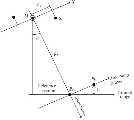
Figure1: Geometrical schematization of the problem under study. AnN-sensor array receives signal from two (or more) sources.B andxare cross-range coplanar axes normal to the azimuth direction (see alsoFigure 2).

wherev(P) is the velocity of the scattering centre within the resolution cell.

From the above considerations, we can finally write the model of the interferometric phase of each interferogram:

φP,t_i=Ci

vv(P) +CDEMi ε(P) +η

P,t_i, i=1,. . .,N. (4)

As discussed in [12,13], the two unknown parametersvand

εcan be estimated jointly maximizing the (first-order) phase coherence function:

γI(P)= _N1

N

i=1

ejφdata,ie−jφmodel,i

, (5)

whereφmodel,iis computed according to (4). Coherence val-ues range from 0 to 1 as a function of the dispersion of the phase residues with respect to the model (η). From (5) it is clear that no use of the amplitude data is present in the esti-mation ofvandεin standard PS analysis.

2.2. Second-order model

We will now discuss the case of two dominant scatterers within the same resolution cell. This yields a second-order model, first outlined in [25]. The mathematical framework can be made very similar to that adopted in direction of ar-rival (DOA) analyses (see [23,24,26] and references therein). The multibaseline dataset relative to pixelPcan be viewed as a snapshot of a nonuniform array composed of N sensors (Figures1and2).

HereX,x, andR_Mare coplanar axes belonging to a plane normal to the satellite trajectories (related to the azimuth di-rection) and passing through the resolution cell under study.

(4)

Bj

M

X

Si

θ

RM

P0 P0

Pk

εk

Reference elevation

Slant

range

Crossrange

x-axis

Ground range

Figure2: SAR acquisition geometry.Mis the master antenna,Sthe slave. Parallel baseline components do not impact the mathematical modelling for phase variations.P0represents the reference DEM for the pixel under analysis.Pis the dominant scattering-centre within the resolution cell.

topography (i.e., reference DEM). The complex signal re-ceived by theith sensor can be modeled as

si=z1ej(4π/λ)r(Bi,ti,x1)+z2ej(4π/λ)r(Bi,ti,x2), (6)

where the dependency of the range coordinate on the normal baselineB_i, the temporal baselinet_i, and the cross-range po-sitionx_kof scattererkhas been highlighted, andz1andz2are

the complex reflectivities of the two scattering centres. For the sake of simplicity, in this paper we will suppose thatall scatterers within the same resolution cell are aﬀected by

the same displacement. In particular, considering the constant

velocity model, we will suppose

v1=v2=v. (7)

FromFigure 1it is easy to verify that

rki=rBi,ti,xk=

R2

M+Bi−xk2

∼ =RM+

Bi−xk2

2RM , k=1, 2,

(8)

where the approximation is valid for satellite sensors (typi-callyR_M > 800 km and|B| < 2 km). In particular, for the master acquisition, we have

rkM∼=RM+ x 2 k

2R_M, k=1, 2. (9)

If now we define the diﬀerential interferogram as

yi≡ sMs ∗ i

_s_Me−j(4π/λ)(RM−Ri) ₍₁₀₎

(wheres∗ is the complex conjugate ofs), the absolute value of the interferogram equals the amplitude of the slave image and it is easy to demonstrate (see the appendix) that (2), (6), (8), (9), and (10), jointly with hypothesis (7), lead to the ex-pression

yi=β1ej(A i DEMx1−Ci

vv)₊β₂ej(AiDEMx2−Cviv)_, i₌_1,. . ._,N_{, (11)}

where

β1= _z₁2

+z2z∗1ej(4π/λ)(x 2 2−x2_1/R

M)

_s_M_| ,

β2= _z₂2

+z1z∗2ej(4π/λ)(x 2 1−x2_2/R

M)

_s_M .

(12)

It is worth noting that

_β₁2 =z1

2

, β2 2

=z2 2

. (13)

Moreover, sincex=ε/sinθ(Figure 2), system (11) can also be written as

yi=β1ej(C i DEMε1−Ci

vv)₊_β 2ej(C

i DEMε2−Ci

vv)_. ₍₁₄₎

Equations (11) and (12) show that, by introducing a second-order model for the scattering and a constant velocity model for target displacement, data can be modelled as thesum of

two complex sinusoidscharacterized by 5 unknown

parame-ters (3 real and 2 complex variables) to be estimated by the dataset available:v,x1,x2,β1,β2.

2.3. Higher-order models

The generalization to higher-order models is straightfor-ward. In general, for a scattering model of order K, where

xkis the position of thekth target on thex-axis inFigure 1 (k=1,. . .,K), we can generalize expression (11) as follows:

yi=e−jCivv _K

m=1

βmejAiDEMxk

, (15)

where

βm=_s1 M

K

l=1

zlz∗mej(4π/λ)(x 2

l−x2m/2RM)_. ₍₁₆₎

(5)

3. INVERSE PROBLEM SOLUTION

As discussed in the previous section, the adoption of a second-order model for PS analysis introduces three further unknown parameters with respect to the standard approach, even considering scatterers aﬀected by the same displace-ment. In order to estimate v,x1,x2,β1,β2, the nonlinear

model (11) needs to be inverted on a pixel-by-pixel basis. Although most of the procedures used in DOA problems re-quire uniform array [23,24,26,27,28], many algorithms can be applied to solve this problem. Here we adopt the nonlin-ear least squares method (NLSM) presented in [27], since it turned out to be robust and eﬀective for the problem under study. However, future research eﬀorts will address the se-lection of the best inversion algorithm for real data, taking into account accuracy, precision, robustness performance, as well as the related computational load. Letθbe ap×1 vec-tor of unknown parameters,x(θ) the model (N-dimensional nonlinear function of the parameters vector), andythe data vector. As is well known, the object function used in NLSM is

J=y−x(θ)Hy−x(θ). (17)

For the problem under study we have

x(m)= n

k=1

αkej(ωkm+ϕk). (18)

In order to recover the unknown pulse frequencies{ωk} ∈ [−π,π], amplitudes {αk}, and initial phases {ϕk} starting from the observed datay, the following cost function has to be minimized:

J=N

i=1 yi−

n

k=1

αkej(ωki+ϕk) 2

. (19)

We now introduce the following notation [27]:

βk=αkejϕk, β=β1· · ·βn T,

(20)

B=

     

ejω1 _{· · ·} _ejωn ..

. ...

ejNω1 _{· · ·} _ejNωn     

. (21)

The model is then linear inβand nonlinear inω:

x=Bβ, (22)

and the cost function is now

J=(Y−Bβ)H(Y−Bβ), (23)

where Y = [y(1)· · ·y(N)]T.Bis a Vandermonde matrix that fulfils the following rank property:

rank(B)=n ifN≥n, ωk=ωp fork=p. (24)

If conditions (24) are met, the matrix (BHB)−1 _{exists and}

(23) yields

J=β−BHB−1BHY HBHB β−BHB−1BHY

+YHY−YHBBHB−1BHY. (25)

For each choice of ω = [ω1,. . .,ωn]T in B (with ωk =

ωpfork = p) a vectorβthat cancels the first term of (25) can be found. Vectorsβandωminimizing expression (25) are therefore,

ω=argmax ω

YHBBHB−1BHY , (26)

β=BHB−1BHY|_ω=ω. (27)

The application of the NLSM to system (11) leads to the fol-lowing cost function:

J=

N

i=1 yi−

2

k=1

βkejωki 2

, (28)

whereβ_kis defined by (12),ω_k_i=Ci

DEMεk+Cviv, andNis the

number of data available.Bis then an (N×2) matrix:

B=

    

ej(C1_DEMε1−C1

vv) ej(C1DEMε2−Cviv) ..

. ...

ej(CNDEMε1−CvNv) _ej(CDEMε2−CN Nvv)    

. (29)

For each matrix B expression (26) must be evaluated and the values (ε1,ε2,v) maximizing it are the solution.Figure 3

shows an example of target function to be maximized in (26): local maxima are present (the problem is strongly nonlinear), but whenever the signal-to-noise ratio (SNR) is high enough and the underlying model fits the data, the global maximum is well pronounced.

Once we have estimated deformation rate and elevations of the scatterers, we can estimateβ1andβ2via (27). The

es-timated valuesv,ε1,ε2,β1,β2can then be used to build

yi=β1ej(C i

DEMε1−C ivvˆ)₊β₂ej(CiDEMε2−Cvivˆ)_, i=_1,. . ._,N_{, (30)}

and to define the “second-order phase coherence,” natural extension of the first-order coherence (5):

γII(P)=_N1 N

i=1

ejφdata,i_e−j∠yˆi_, ₍₃₁₎

where∠yˆ_iis the phase value of expression (30). Similarly to

(6)

120 100 80 60 40 20 0

Ta

rg

et

fu

n

ct

io

n

50 30

10 −10

−30 −50 ε1

−50 −30 −10

10 30

50 ε2

Figure3: Example of target function to be maximized in (26). For visualization purposes, the velocity parameter is fixed to the opti-mum value whileε1andε2vary in the range [−50, 50] meters. This is a real data example, referring to the dataset analysed inSection 5. The two maxima (the function is symmetric) are easily detectable.

residues rather than the LMS error between the complex data vector and the model. This is not unreasonable whenever the final target of the analysis is the extraction of precise displace-ment time series (related to phase data) rather than the char-acterization of local reflectivity. Of course, since the compu-tational load of this optimization is proportional to the vol-ume of the three-dimensional parameter space in which the unknownsv,ε1,ε2can vary (plausibility region), the number

of operations per pixel is much higher than in conventional PS analysis, where a portion of a two-dimensional space is spanned by the estimation algorithm [12,13].

The solutionε1=ε2causes the productBHBto be a

sin-gular matrix and expression (26) will diverge. Thus, the case of a single scatterer will not be solved by the second-order model as two coinciding scattering centres but the first-order scatterer will be split into a dominant scatterer and a second very low-reflectivity centre. This yields an overblown solu-tion which causes

γII(P)< γI(P). (32)

The pixel will consequently be considered a first-order scat-terer.

3.1. Model order selection

Common to all parametric analyses, model order selection (MOS) is a key step that should be carefully studied before accepting the results of the estimation. Indeed, although the conditionγ_II > γ_Iis generally satisfied, this does not neces-sarily imply that the second order is a better model for the data.

As well known, one of the most diﬃcult and critical issues facing sensor arrays systems is the detection of the number of sources impinging on the array [26]. Problems of model

order selection are usually faced based on the Akaike infor-mation criteria [29] or the Rissanen minimum description length criteria [30].

It should be noted that a simple MOS strategy such as the computation of the periodogram for each pixel, looking for the number of maxima, would not be successful, due to resolution limits. In fact, two nearby scattering centres (just a few meters apart) are not detectable by nonparametric ap-proaches.

By limiting the analysis on first- and second-order mod-els only (the estimation is to be carried out on millions of pixels in a typical SAR scene and so the computational bur-den is a key issue for applications), the problem can be cast as a hypothesis testing procedure. In fact, we can formulate two mutually exclusive options for the scattering mechanism:

H0: resolution cellPcontains one scattering-centre,

H1: resolution cellPcontains two (or more)

scattering-centres.

In other words, after first-andsecond-order analysis, we have to establish whether or notH1can be accepted, fixing a

confi-dence level for the decision. In general, in order to limit over-fitting,H1hypothesis should be accepted (or analogouslyH0

should be rejected) only if the probability that the data vec-tor comes from a single scattering centre is below a certain threshold THR, that is, if

PrH0|data

<THR=⇒H1. (33)

The key issue is then the definition of the rejection region. In-tuitively, one should acceptH1only “if it is worth,” for

exam-ple, if the dispersion of the phase residues is significantly re-duced adopting a more complex model, or—equivalently— if the gain in phase coherence is high enough. Although an analytical analysis is very complex, a possible solution can be achieved using a Monte Carlo approach, discussed in the next section.

4. NUMERICAL SIMULATION

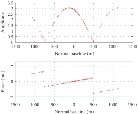
First- and second-order estimation algorithms were tested first on simulated numerical data at diﬀerent levels of signal-to-noise ratio (SNR). The simulation allows one to better appreciate the limits related to the first-order model. Two data vectors are reported in Figures 3and4. In both cases two motionless scattering centres are considered (v=0 and

H1 = true). The baseline distribution used in the

simula-tion resembles that of the real dataset available, described in Section 5. No noise is present in these examples, so the data satisfy (11), (12), and (13).

First we notice that whenever two identical scatterers (i.e.,z1 = z2) are present (Figure 4), the first-order model

(7)

3.5 3 2.5 2 1.5 1 0.5 0

−1500 −1000 −500 0 500 1000 1500 Normal baseline (m)

A

m

plitude

π

−π 0

−1500 −1000 −500 0 500 1000 1500 Normal baseline (m)

Phase

(r

ad)

Figure4: Simulated interferometric data (second order). Parame-ters:v=0,x1=15 m,x2= −4 m, and|z1| = |z2|. While amplitude data show significant variations, phase values can be fitted using a first-order model.

or in general a homogeneous flat (with respect to the illu-minating wavelength) surface can be well described by the model used in conventional PS analysis and SAR interferom-etry (at least limiting the analysis tophase values). On the contrary, whenever the energy backscattered by the radar tar-gets within the resolution cell is not exactly the same (and none of them dominates the scenario), a distortion of the lin-ear phase trend is introduced and the first-order model may fail to model the data correctly (Figure 5). The phase distor-tion is a funcdistor-tion of the normal baseline distribudistor-tion of the dataset, the distance between the two scattering centres, and the ratio of the two reflectivity amplitudes.

In general, working on real data, higher-order scattering models should better describe the reflectivity of the image pixels, however their eﬀectiveness depends very much on the distribution of the baseline values, the extension of the reso-lution cell, and the characteristics of the area of interest.

4.1. Monte Carlo determination of the rejection region

Apart from testing the implementation of the two algo-rithms for data analysis, numerical simulations were used to determine the rejection region for model order selection (Section 3.1).

As already mentioned, a reasonable criteria is to accept

H1(i.e., the double-scatterer model) only if the dispersion of

the phase residues is significantly reduced passing from the first- to the second-order model, that is, running the NLSM on the data. For Gaussian distribution of the phase residues, it can be demonstrated that [14]

γq=e−σq2/2, q=I,II, (34)

whereσ_Iandσ_IIare the dispersion of the phase residues with respect to the model adopted. Therefore, the rejection region can be determined using either (σ_I,σ_II) or (γ_I,γ_II).

3.5 3 2.5 2 1.5 1 0.5 0

A

m

plitude

π

−π 0

Phase

(r

ad)

Figure5: Simulated interferometric data (second order). Parame-ters:v=0,x1=15 m,x2= −4 m, and|z1| = |z2|. The distortion of the phase values with respect to a data vector generated by a single dominant scatterer (or a homogeneous flat surface) is evident.

A possible operational procedure is then the following. For each of Qdiﬀerent SNR levels, 10M realizations of the data vector (sampled at the baseline values of the dataset un-der study) are created consiun-dering a single scattering centre (H0 = true). The values of (σI,σII) are then estimated for

each realization and a scatterogram is generated. The rejec-tion region at confidence level 10−Mcan then be determined on the (σ_I,σ_II)-plane by delimiting the cluster of points of the simulation by means of a suitable curve that fits best the edge of the cluster. InFigure 6the scatterogram obtained af-ter 120 000 realizations (Q=12,M =4) of the data vector is reported. Since—in general—we are interested in the de-tection of radar targets characterized by low phase dispersion (the PS), we can also impose

σII<THR. (35)

It should be pointed out that the rejection region depends on (1) the number of data available, (2) the distribution of normal baseline values, (3) the parameter space spanned by the estimation algorithms; thus this procedure should be run every time a new dataset has to be processed.

5. REAL DATA ANALYSIS

(8)

1.5

1

0.5

0

0 0.2 0.4 0.6 0.8 1 1.2 1.4 σI

σII

H0

H1

Figure6: Numerical determination of the rejection region for hy-pothesis testing. 120 000 realizations (Q=12,M=4) of the data-vector have been generated and both first- and second-order esti-mation algorithms have been applied.σIandσIIindicate the

stan-dard deviation of the phase residues after the application of the first-and second-order estimation algorithms, respectively. The white area specifies the rejection region whereH0 hypothesis should be rejected.

15 10 5 0 −5

−10

−15 ×102

−20 −15 −10 −5 0 5 10 15 20 25 30 ×102 Temporal baseline (d)

P

er

p

endicular

baseline

(m)

Figure7: Distribution of the geometrical and temporal baseline of the interferometric dataset (SAR data: ESA-ERS. Frame 2691-Track 208).

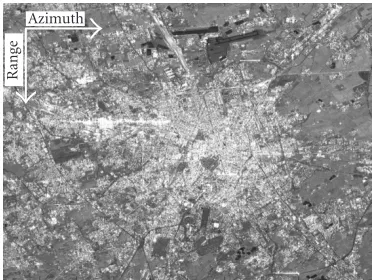
area is a cut out of the whole scene about 40 km2_{wide and}

it is not aﬀected by significant surface deformation phenom-ena, apart from terrain subsidence at low rates (<3 mm/yr) in some suburbs of the city. The constant velocity model is then suitable for the PS analysis. The density of buildings and man-made structures is extremely high, allowing one to get meaningful statistical parameters for PS characterization in urban areas.

Azimuth

Range

Figure8: Incoherent average of the SAR data available over Milano. Eighty-two images acquired by the ESA-ERS sensors have been pro-cessed (Frame 2691-Track 208). The area is heavily urbanized.

1.5

1

0_.5

0

0 0.5 1 1.5

σI σII

H0

H1

Figure9: Scatterogram obtained by processing the Milano dataset superimposed on that obtained from the numerical simulation (Figure 5).

Following the algorithm outlined in the previous sec-tions, we applied both first- and second-order analysis tools for data analysis. In order to limit the computational load, second-order model was used only ifγ_I(P)<0.8 (since oth-erwise the pixel was already labelled as PS) and first-order results (i.e., deformation rate ˆv_I, elevationεI, and the first-order coherence ˆγI) were used to define the portion of the parameter space to be spanned by the NLSM. More precisely, wheneverγ_I(P)>0.6,

vII=vI+α1, α1∈[−0.75, 0.75], ∆v=0.25 mm/yr,

εII,1=εI+α2, α2∈[−20, 20], ∆ε1=0.5 m,

εII,2=εI+α3, α3∈[−20, 20], ∆ε2=0.5 m,

(36)

where∆is the sampling step used in the scanning.

(9)

Figure10: Double-scatterer position (triangular symbols) and sin-gle PS (circular symbol) superimposed on an orthophoto of Milano.

simulation. 38 549 double scatterers were identified (falling in H1) out of 254 226 pixels analysed (15%). It should be

pointed out that since the standard analysis allowed the de-tection of about 200 000 pixels exhibiting ˆγ_I > 0.8 and the increase in PS density by applying the second-order model was about 20%.

After data processing, double-scatterers positions were estimated (using standard geocoding algorithms) and super-imposed on an orthophoto of the area of interest. Two ex-amples are reported in Figures10and11, where the position of the dominant scatterer estimated by the first order analy-sis (circular symbol) has been superimposed to the positions of the two scattering-centres estimated by the second-order model (triangular symbol). In general, all the positions of the scattering-centres turned out to fall within the shape of building and other structures, but of course more in depth analyses should assess the precision of the estimated param-eters.

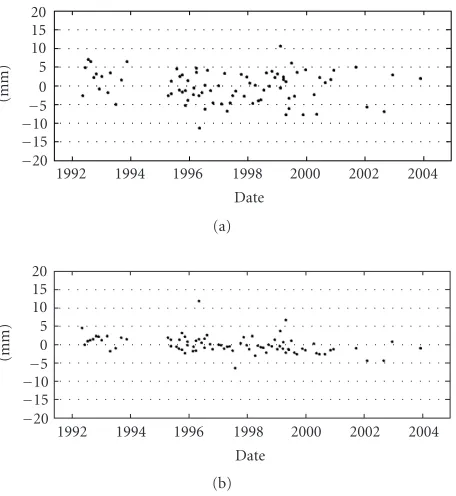
The improvement in data modelling due to the introduc-tion of the second-order model can be appreciated in Figures 12 and13, where the comparison of the two displacement time series relative to scatterers depicted in Figures10and11 is reported.

6. CONCLUSIONS

In this paper we have described a possible strategy to improve the performance of the PS technique, using the same multi-interferogram framework and adopting more complex mod-els for the scattering mechanism within the SAR resolution cell. The preliminary results reported here should be consid-ered only as a first contribution toward a full exploitation of multibaseline satellite datasets characterized by high normal baseline values for surface deformation monitoring.

An important issue to be further studied is the statistical distribution of the cross-range dimension of the PS, both in urban and nonurban areas. In fact, the increase in PS density

Figure11: Double-scatterer position (triangular symbols) and sin-gle PS (circular symbol) superimposed on an orthophoto of Milano.

(20%), although not negligible, could not completely change the scenario obtained by means of the standard PS analysis, at least in the dataset used in this paper (to a certain extent, this justifies the success of the analysis presented in [12,13]). In-deed, since the statistical distribution of the normal baseline values of a typical satellite dataset is far from uniform [14] (within the satellite dead-band), the application of the sim-ple first-order model can be extremely eﬀective. Preliminary results seem to suggest that this kind of algorithms, due to the increased computational load, should be applied only when-ever it is mandatory to extract as much information as pos-sible, pushing the technology to its theoretical limits, or—in general—when the first-order PS distribution is not enough for the application at hand.

Future research activities will be also devoted to the ap-plication of higher-order models to nonurban areas, assess-ing the possibility to resolve layover areas (at least where tem-poral decorrelation is low enough) and the implementation of a more general K-order analysis tool, carefully selecting the best algorithm for the estimation of the unknown param-eters.

Finally, further eﬀorts should be devoted to precision as-sessment, trying to cross-validate, using independent data and possible in situ surveys, the parameters estimated from the multibaseline datasets. Even considering higher-order models, the mathematical framework related to a single mas-ter image, that is, the generation of all inmas-terferogram with re-spect to the same master acquisition, seems to be extremely eﬀective also to get quantitative estimation of precision and accuracy of the unknown geophysical parameters that can be recovered.

APPENDIX

FORMULATION OF THE SECOND-ORDER MODEL

(10)

20 15 10 5 0 −5 −10 −15 −20

(mm)

1992 1994 1996 1998 2000 2002 2004 Date

(a) 20

15 10 5 0 −5 −10 −15 −20

(mm)

1992 1994 1996 1998 2000 2002 2004 Date

(b)

Figure12: Comparison of the displacement time series estimated by applying (a) first- and (b) second-order models for the PS (double-scatterer) highlighted inFigure 9.γI=0.62, γII=0.87.

framework similar to the one used in the direction-of-arrival analysis [23,24,26].

Adopting the first Born approximation (and considering valid the superposition of the eﬀects), the signal received by theith sensor (i=1,. . .,N) can be written as

si=z1j(4π/λ)r1iejC i

vv₊zj(4π/λ)r2i

2 ejC

i

vv_, _(A.1)

rkibeing the target-sensor distance,zkthe complex reflectiv-ity of thekth scattering centre (k =1, 2), andCi_v =4πt_i/λ. wheretiis theith the temporal baseline.

FromFigure 1, the approximated target-sensor distance

rkireads

rki=rBi,ti,xk=

R2

M+Bi−xk2

∼ =RM+

Bi−xk2

2RM , k=1, 2.

(A.2)

Moreover, hypothesis (7) remarks that all the scatterers within the same resolution cell are supposed to be aﬀected by the same displacement:

v1=v2=v. (A.3)

The backscattered signal acquired by the master acquisition and theith slave acquisition yields to the computation of the

20 15 10 5 0 −5 −10 −15 −20

(mm)

1992 1994 1996 1998 2000 2002 2004 Date

(a) 20

15 10 5 0 −5 −10 −15 −20

(mm)

1992 1994 1996 1998 2000 2002 2004 Date

(b)

Figure13: Comparison of the displacement time series estimated by applying (a) first- and (b) second-order models for the PS (double-scatterer) highlighted inFigure 12.γI=0.66,γII=0.90.

ith interferogramYi(divided by the amplitude of the master scene) as

Yi= sMs ∗ i _s_M

= e−jC

i vv _s_M_z₁2

ej(4π/λ)((Bnix1/RM)−(B2 ni/2RM))

+z1z∗2ej(4π/λ)((x 2

1/2RM)−(x_2/2₂_R

M)+(Bnix2/RM)−(B2 ni/2RM))

+z∗₁z2ej(4π/λ)((x 2

2/2RM)−(x_1/2₂_R

M)+(Bnix1/RM)−(B2 ni/2RM))

+z2 2

ej(4π/λ)((Bnix2/RM)−(B2 ni/2RM))_.

(A.4)

Theith diﬀerential interferogram (computed using the a pri-ori elevation x = 0—Figure 2) is then obtained by the fol-lowing expression:

yi≡ sMs ∗ i

_s_Me−j(4π/λ)(RM−Ri)₌_Y

ie−j(4π/λ)(RM−Ri), (A.5)

with

Ri=

R2

M+B2ni∼=RM+

B2 ni

(11)

where the approximation is valid for satellite sensors (R_M > 800 km and|B|<2 km).

By substitution of (A.4) and (A.6) in (A.5) and using relation (2),

yi=e−jCivvejAiDEMx1 z1 2

+z2z1∗ej(4π/λ)(x 2 2−x_1/2₂_R

M) _s_M

+e−jCivvejAiDEMx2 z2 2

+z1z2∗ej(4π/λ)(x 2 1−x_2/2₂_R

M) _s_M

.

(A.7)

Now we define the complex expressionsβ1andβ2as follows:

β1= _z₁2

+z2z∗1ej(4π/λ)(x 2 2−x2_1/R

M)

_s_M ,

β2= _z₂2

+z1z∗2ej(4π/λ)(x 2 1−x2_2/R

M)

_s_M .

(A.8)

Using now (A.8) in (A.7) we finally obtain the definition of

thesecond-order modelof the diﬀerentials:

yi=β1ej(A i DEMx1−Ci

vv)₊β₂ej(AiDEMx2−Cviv)

=β1ej(C i

DEMε1−C_vi_v₎

+β2ej(C i DEMε2−Ci_v_v₎

, i=1,. . .,N, (A.9)

wherex=ε/sinθandAi_DEM=Ci

DEMsinθ.

Starting from (A.8) and computing expressions (A.1) and (A.2) for the master acquisition (C_vM =0, witht_M =0, and

BM=0), it can be demonstrated that

_β₁2 =z1

2

z1 2

+z2 2

+ 2z1z2cosξ _z₁2

+z22+ 2z1z2cosξ

=z12,

(A.10)

whereξ=(4π/λ)(x2

2−x21/2RM) +∆ψ, with∆ψthe diﬀerence

between the two scatterers reflectivity phases. Similarly, for

β2,

_β₂2 =z2

2_z

22+z12+ 2z1z2cosξ) _z₂2

+z1 2

+ 2z1z2cosξ

=z22.

(A.11)

Equations (A.8) and (A.9) correspond to the second-order model described inSection 2.2through (12) and (14).

ACKNOWLEDGMENTS

Authors wish to thank the whole technical staﬀof TRE for the implementation of the algorithms described in this pa-per. This research was self-financed by TRE and Politecnico di Milano.

REFERENCES

[1] A. K. Gabriel, R. M. Goldstein, and H. A. Zebker, “Mapping small elevation changes over large areas: diﬀerential radar in-terferometry,”Journal of Geophysical Research, vol. 94, no. B7, pp. 9183–9191, 1989.

[2] D. Massonnet and K. L. Feigl, “Radar interferometry and its application to changes in the earth’s surface,”Reviews of Geo-physics, vol. 36, no. 4, pp. 441–500, 1998.

[3] P. A. Rosen, S. Hensley, I. R. Joughin, et al., “Synthetic aper-ture radar interferometry,”Proc. IEEE, vol. 88, no. 3, pp. 333– 382, 2000.

[4] R. B¨urgmann, P. A. Rosen, and E. J. Fielding, “Synthetic aper-ture radar interferometry to measure Earth’s surface topogra-phy and its deformation,”Annual Review of Earth and Plane-tary Sciences, vol. 28, pp. 169–209, May 2000.

[5] R. F. Hanssen,Radar Interferometry: Data Interpretation and Error Analysis, Kluwer Academic, Dordrecht, the Netherlands, 2001.

[6] S. Madsen, H. A. Zebker, and J. Martin, “Topographic map-ping using radar interferometry: processing techniques,”IEEE Trans. Geosci. Remote Sensing, vol. 31, no. 1, pp. 246–256, 1993.

[7] D. Massonnet, P. Briole, and A. Arnaud, “Deflation of Mount Etna monitored by spaceborne radar interferometry,”Nature, vol. 375, no. 6532, pp. 567–570, 1995.

[8] D. Massonnet, K. L. Feigl, M. Rossi, and F. Adragna, “Radar interferometric mapping of deformation in the year after the Landers earthquake,”Nature, vol. 369, no. 6477, pp. 227–230, 1994.

[9] D. Massonnet, W. Thatcher, and H. Vadon, “Detection of postseismic fault-zone collapse following the Landers earth-quake,”Nature, vol. 382, no. 6592, pp. 612–616, 1996. [10] G. Peltzer and P. A. Rosen, “Surface displacement of the 17

May 1993 Eureka Valley, California earthquake observed by SAR interferometry,”Science, vol. 268, pp. 1333–1336, 1995. [11] H. A. Zebker and J. Villasenor, “Decorrelation in

interfer-ometric radar echoes,”IEEE Trans. Geosci. Remote Sensing, vol. 30, no. 5, pp. 950–959, 1992.

[12] A. Ferretti, C. Prati, and F. Rocca, “Permanent scatterers in SAR interferometry,”IEEE Trans. Geosci. Remote Sensing, vol. 39, no. 1, pp. 8–20, 2001.

[13] A. Ferretti, C. Prati, and F. Rocca, “Nonlinear subsidence rate estimation using permanent scatterers in diﬀerential SAR in-terferometry,” IEEE Trans. Geosci. Remote Sensing, vol. 38, no. 5, pp. 2202–2212, 2000.

[14] C. Colesanti, A. Ferretti, F. Novali, C. Prati, and F. Rocca, “SAR monitoring of progressive and seasonal ground de-formation using the permanent scatterers technique,”IEEE Trans. Geosci. Remote Sensing, vol. 41, no. 7, pp. 1685–1701, 2003.

[15] P. Berardino, G. Fornaro, R. Lanari, and E. Sansosti, “A new algorithm for surface deformation monitoring based on small baseline diﬀerential SAR interferograms,”IEEE Trans. Geosci. Remote Sensing, vol. 40, no. 11, pp. 2375–2383, 2002. [16] O. Mora, J. J. Mallorqui, and A. Broquetas, “Linear and

non-linear terrain deformation maps from a reduced set of inter-ferometric SAR images,”IEEE Trans. Geosci. Remote Sensing, vol. 41, no. 10, pp. 2243–2253, 2003.

[17] S. Usai, “A least squares database approach for SAR interfero-metric data,”IEEE Trans. Geosci. Remote Sensing, vol. 41, no. 4, pp. 753–760, 2003.

(12)

[19] S. Salvi, S. Atzori, C. Tolomei, et al., “Inflation rate of the Colli Albani volcanic complex retrieved by the permanent scatter-ers SAR interferometry technique,”Geophysical Research Let-ters, vol. 31, no. 21, 2004.

[20] G. E. Hilley, R. B¨urgmann, A. Ferretti, F. Novali, and F. Rocca, “Dynamic of slow-moving landslides from permanent scat-terer analysis,” Science, vol. 304, no. 5679, pp. 1952–1955, 2004.

[21] A. Reigber and A. Moreira, “First demonstration of airborne SAR tomography using multibaseline L-band data,” IEEE Trans. Geosci. Remote Sensing, vol. 38, no. 5, pp. 2142–2152, 2000.

[22] C. R. Smith and P. M. Goggans, “RADAR target identifica-tion,”IEEE Antennas Propagat. Mag., vol. 35, no. 2, pp. 27–38, 1993.

[23] F. Gini, F. Lombardini, and M. Montanari, “Layover solu-tion in multibaseline SAR interferometry,”IEEE Trans. Aerosp. Electron. Syst., vol. 38, no. 4, pp. 1344–1356, 2002.

[24] F. Lombardini, M. Montanari, and F. Gini, “Reflectivity estimation for multibaseline interferometric radar imaging of layover extended sources,”IEEE Trans. Signal Processing, vol. 51, no. 6, pp. 1508–1519, 2003.

[25] M. Lorenzi and D. Magni, “Sviluppi della tecnica dei Bersagli Permanenti,” M. Sc. Thesis, Politecnico di Milano University, Milano, Italy, 2001.

[26] H. Krim and M. Viberg, “Two decades of array signal process-ing research: the parametric approach,”IEEE Signal Processing Mag., vol. 13, no. 4, pp. 67–94, 1996.

[27] P. Stoica and R. L. Moses,Introduction to Spectral Analysis, Prentice-Hall, Englewood Cliﬀs, NJ, USA, 1997.

[28] S. M. Kay,Fundamentals of Statistical Signal Processing, Vol-ume I: Estimation Theory, Prentice-Hall, Englewood Cliﬀs, NJ, USA, 1993.

[29] H. Akaike, “Information theory and an extension of the max-imum likelihood principle,” inProc. IEEE 2nd International Symposium on Information Theory, B. N. Petrov and F. Caski, Eds., pp. 267–281, Akademiai Kiado, Ashkelon, Israel, June 1973.

[30] J. Rissanen, “Modelling by the shortest data description,” Au-tomatica, vol. 14, no. 5, pp. 465–471, 1978.

Alessandro Ferretti was born in Milano, Italy, on January 27, 1968. He received the degree in electrical engineering (cum laude) from Politecnico di Milano (POLIMI) in 1993 and the M.S. degree in information technology (cum laude) from CEFRIEL. In May 1994 he joined the POLIMI Radar Group working on SAR interferometry. In July 1997, he received the Ph.D. degree in electrical engineering from POLIMI. After

devoting most of his research efforts to multitemporal SAR data stacks at the Department of Electronics, he developed together with Professors Rocca and Prati what is now called the “perma-nent scatterer technique,” a technology patented in 1999 that can overcome most of the difficulties encountered in conventional SAR interferometry. In March 2000 he founded, together with Profes-sors Rocca and Prati, and Politecnico di Milano the company Tele-Rilevamento Europa (TRE), the first POLIMI spin-off, where he is currently the Managing Director. Dr. Ferretti has been involved in many projects financed by the European Space Agency and was the promoter, in 2003, of the first interferometric archive of Radarsat data on a national level. His research interests include radar data processing, optimization algorithms, data fusion, and the use of re-mote sensing information for civil protection applications.

Marco Bianchiwas born in 1978 in Busto Arsizio, Italy. He received a Laurea degree in telecommunication engineering from Po-litecnico di Milano (POLIMI) in 2003 with a study about phase ambiguity estimation in SAR interferometry developed at Delft Uni-versity of Technology, The Netherlands. In the same year, he joined Tele-Rilevamento Europa, Milano, Italy, working on the per-manent scatterers technique, mainly

focus-ing his research activity on the higher-order models for PS analysis.

Claudio Prati was born in Milano on March 20, 1958. He is Full Professor of telecommunications at the Electronic De-partment, Politecnico di Milano. He holds three patents on the SAR images process-ing. He has been awarded two prizes from the IEEE Geoscience and Remote Sensing Society (IGARSS’89 and IGARSS’99). He published more than 100 papers on SAR data processing and interferometry. He is

cofounder of Tele-Rilevamento Europa (TRE), an RS spin-oﬀ com-pany of POLIMI.

Fabio Roccareceived his degree in electri-cal engineering in 1962. He is a Professor of digital signal processing at Politecnico di Milano. He dedicated his research to dig-ital signal processing for television band-width compression, emission tomography, seismic data processing, and SAR. He was a Visiting Professor at Stanford University several times from 1978 to 1987/88, De-partment Chairman in 1975–1978,