Volume 2007, Article ID 90727,16pages doi:10.1155/2007/90727
Research Article
Sparse Approximation of Images Inspired from the Functional
Architecture of the Primary Visual Areas
Sylvain Fischer,1, 2Rafael Redondo,1Laurent Perrinet,2and Gabriel Crist ´obal1
1Instituto de ´Optica - CSIC, Serrano 121, 28006 Madrid, Spain
2INCM, UMR 6193, CNRS and Aix-Marseille University, 31 chemin Joseph Aiguier, 13402 Marseille Cedex 20, France
Received 1 December 2005; Revised 7 September 2006; Accepted 18 September 2006
Recommended by Javier Portilla
Several drawbacks of critically sampled wavelets can be solved by overcomplete multiresolution transforms and sparse approxima-tion algorithms. Facing the difficulty to optimize such nonorthogonal and nonlinear transforms, we implement a sparse approx-imation scheme inspired from the functional architecture of the primary visual cortex. The scheme models simple and complex cell receptive fields through log-Gabor wavelets. The model also incorporates inhibition and facilitation interactions between neighboring cells. Functionally these interactions allow to extract edges and ridges, providing an edge-based approximation of the visual information. The edge coefficients are shown sufficient for closely reconstructing the images, while contour representations by means of chains of edges reduce the information redundancy for approaching image compression. Additionally, the ability to segregate the edges from the noise is employed for image restoration.
Copyright © 2007 Sylvain Fischer et al. This is an open access article distributed under the Creative Commons Attribution License, which permits unrestricted use, distribution, and reproduction in any medium, provided the original work is properly cited.
1. INTRODUCTION
Recent works on multiresolution transforms showed the ne-cessity of using overcomplete transformations to solve draw-backs of (bi-)orthogonal wavelets, namely their lack of shift invariance, the aliasing between subbands, their poor resolu-tion in orientaresolu-tion and their insufficient match with image features [1–4]. Nevertheless the representations from linear overcomplete transforms are highly redundant and conse-quently inefficient for such tasks needing sparseness as, for example, for image compression. Severalsparse approxima-tion algorithms have been proposed to address this prob-lem by approximating the images through a reduced num-ber of decomposition functions chosen in an overcomplete set called dictionary [5–8] (see reviews in [6,9]). In some very particular cases there exist algorithms achieving the op-timal solutions. In the general case, two main classes of al-gorithms are available: matching pursuit (MP) [5,10] which recursively chooses the most relevant coefficients in all the dictionary and basis pursuit (BP) [6] which minimizes a pe-nalizing function corresponding to the sum of the amplitude of all coefficients. Both these algorithms perform iteratively and globally through all the dictionary. They are computa-tionally costly algorithms which generally only achieve ap-proximations of the optimal solutions.
We propose here to build a new method for sparse ap-proximation of natural images based both on classical image processing criteria and on the known physiology of the pri-mary visual cortex (V1) of primates. The rationale behind the biological modeling is the plausibility that V1 could ac-complish an efficient coding of the visual information and a certain number of similarities between V1 architecture and recent image processing algorithms: first, the receptive field (RF) of V1 simple cells can be modeled through oriented Gabor-like functions [11], arranged in a multiscale structure [12], similarly to the Gabor-like multiresolutions. Second, V1 supposedly carries out a sparse approximation procedure [13]. And finally, interactions between V1 cells such as in-hibitions between neighboring cells and facilitation between coaligned and collinear cells have been described by physi-ological and psychophysical studies [14–16]. These interac-tions have been shown efficient for image processing in ap-plications such as contour extraction and image restoration [17–21]. We propose here the hypothesis that lateral inter-actions deal not only with contour extraction or noise seg-regation but also allow to achieve sparse approximations of natural images.
Original image
V1 cell receptive
fields
Log-Gabor wavelets
V1 cell non-linearities
Sparse approximation: - Thresholding - Inhibition - Facilitation - Gain control - Quantization
V1 to V4 contour representation
Chain coder: - Endpoints - Mouvements
Reconstructed image
Reconstruction
- Chain decoder - Inverse log-Gabor wavelets
Figure1: Scheme of the algorithm. The lossy parts, that is, the operations inducing information losses, are depicted with gray color.
popular method, and it was shown that overcomplete trans-forms which preserve the translation invariant property are more efficient than (bi-)orthogonal wavelets [1,22]. An aug-mented resolution in orientation was also shown to be im-portant [4], as well as a better match between edges of nat-ural images and the wavelet shape [4]. According to such studies we previously proposed log-Gabor wavelets as a can-didate for an efficient noise segregation [23, 24]. Denois-ing was also shown to be improved by takDenois-ing into account the adjacent neighborhood of transform coefficients [25] or thanks to inhibition/facilitation interactions [17]. Denois-ing is also known to be linked with compression, where (bi-)orthogonal wavelets are the golden standard with JPEG-2000. A compression based on edge extraction was proposed by Mallat and Zhang [26], while the possibility to reconstruct images from their edges was studied in [27]. Several authors proposed a separated coding of edges and residual textures generally by means of sparse approximation algorithms [28–
30]. Various usual and popular edge extraction methods pro-ceed through a first step of filtering through oriented kernels before applying an oriented inhibition or nonlocal maxima suppression and some hysteresis or facilitation processes to reinforce coaligned edge segments [17,19,20,31].
We propose here a unified algorithm for denoising, edge extraction, and image compression based on a new sparse approximation strategy for natural images. The second ob-jective of this study is to approach visual cortex understand-ing and image processunderstand-ing. From the image processunderstand-ing point of view, one important novelty consists in achieving denois-ing and sparse approximation based on multiscale edge ex-traction. From the mathematical point of view, the selection of the sparse subdictionary through local operations and in a noniterative manner is an important novelty. Compared with our previous work implementing oriented inhibition on log-Gabor wavelets [8], the improvements consist here in the implementation of facilitative interactions and in proposing a further redundancy reduction through a contour encod-ing. From the neuroscience point of view, the model aims at reproducing some of the behaviors observed in the visual cortex and to fix the unknown parameters thanks to image processing criteria (this last optimization takes sense since we consider the visual cortex as an efficient visual processing system optimized under evolutionary pressure). It proposes
Inhibition Facilitation
Figure 2: Schematic structure of the primary visual cortex im-plemented in the present study. Simple cortical cells are mod-eled through log-Gabor functions. They are organized in pairs in quadrature of phase (dark-gray circles). For each position the set of different orientations compose a pinwheel (large light-gray cir-cles). The retinotopic organization induces that adjacent spatial po-sitions are arranged in adjacent pinwheels. Inhibition interactions occur towards the closest adjacent positions which are in the direc-tions perpendicular to the cell preferred orientation and toward ad-jacent orientations (light-red connections). Facilitation occurs to-wards coaligned cells up to a larger distance (dark-blue connec-tions).
Table1: Correspondences between visual cortex physiology and image processing operations defined in the different sections.
Visual cortex structures Image processing Section Simple and complex cells log-Gabor fcts.
Section 2.1
Even-sym. simple cell (h(x,y,s,r)) Odd-sym. simple cell (h(x,y,s,r)) Pair of simple cells h(x,y,s,r) Complex cell |h|(x,y,s,r)
Pinwheel h(x,y,s,·)
Retinotopic organization x,yarrangement
Spike threshold CSF (h2) Section 2.2
Oriented inhibition Edges (h3) Section 2.3
Facilitation across scales Parents (f1) Section 2.4
Facilitation across space Chain length (f2) Section 2.5
Set of spiking cells Subdictionaryh4 Section 2.5
Gain control Amplitude (ak) Section 2.6
Hypercomplex cells Endpoints
Section 2.7
Contour shape Movements
Contour representation Chain coding
2. MODEL IMPLEMENTATION
The present study proposes a novel sparse approximation strategy which can at the same time be interpreted as a model of the primary visual areas. The model summarized in Figures 1, 2, and Table 1 also incorporates a contour representation and a reconstruction module. It is composed by successive steps which analyze and integrate the visual information from local features to increasing larger ones. First, simple cell and complex cell receptive fields are mod-eled by log-Gabor functions as described inSection 2.1. Then nonlinear behaviors of V1 cells such as spike thresholding (Section 2.2), inhibition (Section 2.3), facilitation (Sections
2.4and2.5), gain control (Section 2.6) are implemented. Fi-nally a contour representation is proposed inSection 2.7.
2.1. Simple and complex cell receptive fields
The first step of the implementation consists in modeling the receptive fields of the simple cell population through the log-Gabor wavelet transformW which has been proposed in our previous studies [8,23,24]. The transform consists in filtering the given input image x by a set of log-Gabor kernels (G(s,r))(s,r) wheresis the scale which ranges from 1
to 5 for edge extraction and denoising (and from 1 to 6 for compression) andrindexes the orientations ranging from 1 to 6. The scheme also includes a residual low-pass filter. All those kernels are shown inFigure 3for the 5 scales, 6 orien-tation case. Each filter output is called achannel. It represents the response of a set of cells having a particular orientation and scale and covering the full range of positions (eventu-ally decimated for the coarsest scales). The transform coef-ficients are organized in 4-dimensional arrays, called
pyra-mids,h(x,y,s,r) where x, y,s,r denote the position inx, in y, the scale, and the orientation, respectively. h coeffi-cients are complex-valued, the real parts(h) correspond to the receptive fields (RF) of even-symmetric simple cells (i.e., with cosine shape) as shown inFigure 3(b). The imaginary parts (h) correspond to odd-symmetric (i.e., sine shape) RF shown inFigure 3(c). Hence, each coefficient represents
the amplitude of a pair of simple cells in quadrature of phase localized in the same position, orientation, and scale (illus-trated as dark-gray discs inFigure 2). The activities of simple cells are then calculated as (where⊗is the 2D convolution in x,y)
h(x,y,s,r)=G(s,r)(x,y)⊗x(x,y). (1)
The activities|h|of thecomplex cellsare defined as the square quadratic sum of the pairs of simple cells(h) and(h), that is, the modulus of the log-Gabor wavelet coefficientsh. Such definition is consistent with previous models [19,32].
The log-Gabor wavelets are not described in details here, for a thorough study including justifications of their biolog-ical plausibility please refer to [8,23,24]. Nevertheless it is worth stressing here some important characteristics of the log-Gabor wavelets. (1) The transform is linear and is trans-lation invariant. It allows exact reconstruction and is self-invertible (it is a tight frame): the pseudoinverse is also the transposed operator notedWT andWWTx=xfor any im-agex. (2) It is overcomplete by a factorRaround (14/3)nt wherent is the number of orientations (i.e.,R 28 for 6 orientations). Such an overcompleteness factorRis consis-tent with the redundant number of simple cells in compar-ison with the number of photoreceptors in the retina. It is also acceptable for sparse approximation algorithms which currently deal with much more redundant transforms (see, e.g., [28]). (3) The elongated shape and the phase, scale, and orientation arrangement of the filters properly model the re-ceptive fields present in the V1 simple cell population.
2.2. Spike threshold
Those complex cells whose activities do not reach a certain spike rectification threshold are considered as inactive. The contrast sensitivity function (CSF) proposed in [33] is im-plemented here to model this thresholding. CSF(s,r) estab-lishes the threshold of detection for each channel (s,r), that is, the minimum amplitude for a coefficient to be visible for a human observer. All the nonperceptible coefficients are then zeroed out.
In presence of noise, the CSF is known to modify its re-sponse to filter down the highest frequencies (see [34] for a model of such behavior). This change in the CSF is mod-eled here by lowering the spike threshold depending on the noise level. The new threshold level is determined accord-ing to classical image processaccord-ing methodologies for removaccord-ing noise: the noise varianceσ2
(s,r)induced in each channel (s,r)
Low-pass filter
4th scale 5th scale1st scale
2nd scale 3rd scale
(a) Fourier
4
(b) Space (real part)
4
(c) Space (imaginary part)
Figure3: Multiresolution scheme with 6 orientations and 5 scales. (a) Schematic contours of the filters in the Fourier domain. The Fourier domain origin (DC component) is located at the center of the inset and the highest frequencies lie on the border. (b) Real part of the filters in the space domain. Scales are arranged in rows and orientations in columns. The two first scales are drawn at the bottom magnified by a factor of 4 for a better visualization. The low-pass filter is drawn in the upper-left part. (c) The imaginary part of the filters is shown in the same arrangement. The low-pass filter does not have an imaginary part.
apparent noise apart from a few residual noise features. This threshold is set to a low value so as to preserve a larger part of the signal while the processes of facilitation (Sections2.4and
2.5) will refine the denoising by removing the residual arti-facts. The activities of simple cells after spike thresholding are calculated ash2:
h2(x,y,s,r)
=
⎧ ⎪ ⎪ ⎪ ⎪ ⎪ ⎨ ⎪ ⎪ ⎪ ⎪ ⎪ ⎩
h(x,y,s,r)
if|h|(x,y,s,r)≥maxCSF(s,r), 1.85σ(s,r)
,
0 otherwise.
(2)
2.3. Oriented inhibition
The inhibition step is designed according to energy mod-els [19,32] which implement nonlocal maxima suppression between complex cells for extracting edges and ridges. A very similar strategy is also deployed in classical image pro-cessing edge extraction methods like in the Canny operator [31] which marks edges at local maxima after the filtering through oriented kernels. As indicated by the light-gray con-nections inFigure 2the inhibition occurs toward the direc-tion perpendicular to the edge, that is to the filter orienta-tion. It zeroes out the closest adjacent orientations and po-sitions which have lower activity (no inhibition across scales is implemented here). The implementation of the oriented inhibition is not detailed more here since it does not differ substantially from the classical implementations proposed in [19, 31]. The inhibition operation can be summarized by the following equation (where (vx,vy) points to an adjacent pixel in the direction perpendicular to the channel preferred
orientation):
h3(x,y,s,r)
=
⎧ ⎪ ⎪ ⎪ ⎪ ⎪ ⎪ ⎪ ⎪ ⎪ ⎪ ⎪ ⎪ ⎨ ⎪ ⎪ ⎪ ⎪ ⎪ ⎪ ⎪ ⎪ ⎪ ⎪ ⎪ ⎪ ⎩
h2(x,y,s,r)
ifh2(x,y,s,r)
≥ max
(δv,δr)∈{−1,0,1}2 h2
x+δvvx,y+δvvy,s,r+δr,
0 otherwise.
(3)
It is worth to note that the shape of the filter is critical here for an accurately localized, nonredundant and noise-robust detection [31].Figure 4illustrates that log-Gabor fil-ters are adequate for extracting both edges and ridges by non-local maxima suppression: (1) both edges and ridges induce local-maxima in the modulus of the log-Gabor coefficients and (2) that the modulus monotonously decreases on both sides of edges and ridges without creating extra local-maxima (the modulus response is monomodal).
0.2 0
0.2
0.4
0.6
0.8
1
A
m
plitude
15 10 5 0 5 10 15
Position
Norm Real part
Imag. part Signal
(a) Ridge
3 2 1 0 1 2 3 4
A
m
plitude
15 10 5 0 5 10 15
Position
Norm Real part
Imag. part Signal
(b) Edge
Figure4: Log-Gabor wavelet response to edges and ridges. (a) Response of a 1D complex log-Gabor filter to an impulse (ridge): the modulus (black continuous curve) of the response monotonously decreases away from the impulse. It implies that the ridge is situated just on the local maximum of the response. On the contrary the real (dot) and imaginary (dash-dot) parts present various local-maxima and minima which makes them less suitable for ridge localization. (b) Same curves for a step edge.
gaps are cutting offthe contours. Some isolated nonzero co-efficients also remain due to noise as well as irrelevant or less salient edges. Facilitation interactions will now allow to eval-uate the saliency and reliability of such coefficients.
2.4. Facilitation across scales
Facilitation interactions have been described in V1 as ex-citative connections between co-oriented, coaxial, aligned neighboring cells [14,36]. Psychophysical studies and the Gestalt psychology determined that coaligned or cocircu-lar stimuli are more easily detected and more perceptu-ally salient [15,16]. Studies of natural image statistics also show that statistically edges tend to be coaligned and co-circular [37,38]. Experimentally we observe that log-Gabor coefficients arranged in chains of coaligned coefficients or present across different scales correspond to reliable and salient edges. Moreover, the probability that remaining noise features could be responsible for chains of coefficients is de-creasing with the chain length. Thus a facilitation reinforc-ing cocircular cells conforms a noise segregation process. For all those reasons a facilitation across scale is set up to reinforce co-oriented cells across scales (under the condi-tions described in the next paragraph) and a facilitation in space and orientation reinforce chains of coaligned coeffi -cients (Section 2.5).
The facilitation across scales consists in favoring those coefficients located where there exist also noninhibited co-efficients at coarser scales. In practice, theparentcoefficient hp (i.e., the one in the coarser scale) must be located in the same spatial location (tolerating a spatial deviation of one coefficient), in an adjacent orientation channel and be com-patible in phase (i.e., it must have a difference lower than 2π/3 in phase).f1(x,y,s,r)=1 indicates that the coefficient
(x,y,s,r) has a parent (otherwise f1(x,y,s,r) = 0). The
calculation off1can be summarized as follows:
hp(x,y,s,r)= max
(δx,δy,δr)∈{−1,0,1}3h3
x+δx, y+δy,s+1,r+δr,
f1= ⎧ ⎪ ⎪ ⎪ ⎪ ⎨ ⎪ ⎪ ⎪ ⎪ ⎩
1 whereh3=0
andhp=0 and
angleh3,hp< 23π
,
0 elsewhere.
(4)
It is then straightforward to calculate the presence of grand-parents(notedf1(x,y,s,r)=2), where the parent coefficient
has itself a parent.
Kovesi showed that phase congruency of log-Gabor coef-ficients across scales is efficient for extracting edges [39]. It is remarkable to note (seeFigure 5(c)) that many edges and ridges extracted are closely repeated across scales with coeffi-cients linked by parent relationships. This regularity is due in part to the good behavior the log-Gabor wavelets is promis-ing for the decorrelation and efficient coding of contours.
2.5. Facilitation across space and orientation
As proposed in Yen and Finkel’s V1 model [20], we imple-ment a saliency measureimple-ment linked with thechain length
defined as the number of coefficients composing the chain. It is calculated for each coefficient and consists in count-ing the number of coefficients forwardnf and backwardnb
(a) Original image (b) Complex cell activities
(c) Inhibition
(d) Facilitation (e) Reconstruction Figure5: Successive steps modeling V1 architecture as a sparse ap-proximation strategy. (a) 96×96 detail of the “Lena” image. (b) Complex cell activities are modeled as the log-Gabor coefficient modulus (Section 2.1). All the orientations are overlaid so that one inset is shown for each scale. The different scales have different sizes due to the downsampling applied. From the largest to the smallest the insets correspond respectively to the 2nd, 3rd, 4th, low-pass and 5th scale. The first scale is not represented. (c) Remaining coeffi -cients after the inhibition step (Section 2.3). (d) The facilitation step (Sections2.4-2.5) preserves the coefficients arranged in sufficiently long chains and having parent coefficients within coarser scales. The remaining cells conform the sparse approximation of the image. It is composed by a subdictionary including the most salient multiscale edges and the low-pass version of the image. (e) The gain control step (Section 2.6) assigns an amplitude to the subdictionary edges. Then the inverse log-Gabor wavelet transform reconstructs an ap-proximation of the image.
(withlmax =16. The different parameters are chosen
exper-imentally). The saliency is finally calculated in the following form which permits to obtain a constant response along each chain:
f2(x,y,s,r)=min
lmax,nf+nb
. (5)
Finally the facilitation consists in retaining those coeffi-cients which fulfill the following two criteria (while the other coefficients are zeroed out to be considered as noise or less
salient edges). First they must pass a certain length threshold depending of the scale and the presence of parent coefficients. Typically the chain length threshold is chosen as 16, 16, 8, 4, 2, respectively, for the scales 1, 2, 3, 4, 5, half of these lengths if coefficients have a parent, and a fourth of these lengths if they have a grandparent. Second, the amplitude must over-pass a spike threshold corresponding to twice the CSF thresh-old defined inSection 2.2. Each coefficient is selected with its chain neighbors which implies that chains are selected or re-jected entirely (see the final selectionFigure 5(d)). This sec-ond csec-ondition is equivalent to the Canny hysteresis [31]. As a summary, the facilitation process can be approximated by the equation
h4(x,y,s,r)
=
⎧ ⎪ ⎪ ⎪ ⎪ ⎪ ⎨ ⎪ ⎪ ⎪ ⎪ ⎪ ⎩
h3(x,y,s,r) if
f2(x,y,s,r)≥26−s−f1(x,y,r,s)
andh3(x,y,s,r)≥2CSF(s,r)
,
0 otherwise.
(6)
The facilitation implementation is not described here in more detail since it does not incorporate strong improve-ments over the algorithms existing in the literature. More-over small changes in the implementation do not strongly impair the final results.
Both the chain length and CSF thresholds are chosen de-pending on the application since for high compression rates the thresholdings must be severe while for image denoising most edges should be preserved which requires more per-missive thresholds. The first scale edges are less reliable be-cause of the intrinsic lower orientation selectivity of the fil-ters close to the Nyquist frequency. In the present implemen-tation edges selected in the second scale will also be those used for the first scale.
Additionally, for further increasing the sparsity, some co-efficients can be periodically ruled out along chains. If the induced hollows are sufficiently narrow they will not be per-ceptible in the reconstructed image thanks to the important overlapping between log-Gabor functions. This is the case, for instance, when one every two or two every three coeffi -cients are zeroed (as it will be shown inSection 3.2and Fig-ures8,9). This strategy will be exclusively adopted for image compression tasks where highly sparse approximations are required.
2.6. Gain control
In this section both the imagex, the log-Gabor wavelet trans-formh=Wx, and theh4pyramid are treated as 1D vectors
(for such a purpose the 2D or 4D vectors are concatenated into 1D vectors). We have x ∈ RN,h ∈ RM, h4 ∈ RM, W∈RM×N, andWT ∈RN×M,Nbeing the number of pixels
calledsubdictionaryfrom which an approximation of the im-age will be reconstructed. Let us assume D ∈ RM×M the
diagonal matrix defined on the dictionary space and which eigenvalues are 1 on the selected subdictionary and 0 else-where. We calla0=h4theapproximationandr0=h−h4the
residual:
a0=DWx
=h4
, r0=(1−D)Wx
=h−h4
. (7)
The gain control aims at adapting the amplitude of the a0 coefficients for obtaining the closest possible
reconstruc-tion through theWT operation. We know thath =a0+r0
reconstructs exactly the image with WTh = x. Neverthe-less it can be verified experimentally that a0 (the
sparsi-fied version of h) only reconstructs a very smoothed ver-sion ofx: thea0coefficients need to be enhanced for a closer
reconstruction.
This enhancement could be realized through a fixed gain factor. But for a better reconstruction, we adopt a strategy close to matching pursuit [5] which plausibility as biological model has been explored in [7]. MP selects at each iteration the largest coefficient which is added to the approximation while its projection on the other dictionary functions is sub-tracted from theresidual. This projection, which depends on the correlation between dictionary functions, can be inter-preted as a lateral interaction [7]. Here as a difference with MP, the residualr0is projected on the subspaceVspanned by
the subdictionary. We do not know the projection operator P∗that realizes this operation. Thus the projectorP=WWT
that projects the residual on the whole transform space is iteratively used instead1:
ak=ak−1+DPrk−1, rk=(1−D)Prk−1.
(8)
By the self invertible property we haveWTP=WTWWT = WTand it comes that
WTa
k+rk=WTak−1+Prk−1
=WTak−
1+rk−1
. (9)
Iteratively and using again the self-invertible property and (8) we have finally
WTak+rk=WTa
0+r0
=WTWx=x. (10)
Hence,WT(ak+rk) reconstructs exactly the source imagex for anyk.
It is also straightforward to show thatakandrkconverge: letQbe defined asQ=(1−D)P. We have now
ak=a0+DP k
q=1
rq−1=a0+DP
k
q=1
r0,
rk=Qkr0,
(11)
1It is direct thatPis linear andP2=P, hencePis a projector.
P andD being projections, Qe ≤ e for any vectore (where · is the quadratic norm). Moreover any vector ewhich verifiesQe = eis an eigenvector ofP(with
eigenvalue 1) and ofD(with eigenvalue 0), then ofQ(with eigenvalue 1). We deduce that (a)DPQqe =0; and (b) the eigenvalues ofQdifferent than 1 are strictly smaller than 1. Hence for anyr0,DP(
k
q=1Qq)r0andakconverge, and from
(b) we have therkconvergence. The convergence is moreover exponential with a factor corresponding to the highest eigen-value ofQwhich is strictly smaller than 1.
In practice we observe that the algorithm converges with regularity,akandrkbecoming stable in around 40 iterations. If the dictionary has been adequately selected, most of the residual coefficients dramatically decrease their amplitude and the selected coefficients encode almost all the image information (e.g., the reconstruction of Lena is shown in
Figure 5(e)). But because some edges and ridges can lack in the dictionary, in particular around corners, crossing and textures, a second pass of thresholding, inhibition and facil-itation can also be advantageously deployed on the residual for selecting new edge coefficients.
Concerning the overall computational complexity, all the thresholding, inhibition, and facilitation steps are computed by local operations consisting in convolutions by small ker-nels (mainly 3×3). The linear and inverse log-Gabor wavelet transformsWandWT are computed in the Fourier domain but could also be implemented as convolutions in space do-main, which is a biologically plausible implementation. In such a case the algorithm would consist in a fixed number of local operations. The computational complexity would then be as low asO(N), whereNis the number of pixels in the image.
2.7. Contour representation
The former processes allowed to approximate the visual in-formation through continuous chains of active cells repre-senting contour segments (seeFigure 5(d)). The next step in the integration of the visual information would be to build an efficient representation of such chains. For such purpose V1 hypercomplex or end-stopped cells [19, 40,41] which respond preferentially to ridge endings, abrupt corners and other types of junctions and crossings could play an impor-tant role since such features are known to be determinant in perception of contours. Descriptions of integrated con-tours could also take place in higher visual areas like V2 and V4 which are supposed to provide increasingly complex de-scriptions of visual shapes. For instance, recent advances have shown that cells in V4 area may respond to curvature de-gree (concavity) and to angles between aggregated curved segments [42].
implementations a full biological model representing con-tours through shape parameters such as curvatures and an-gles could advantageously be set up.
The contour representation aims at further integrating the visual information simultaneously for providing a de-scription more easily exploitable by the highest visual areas in tasks such as object recognition and for reducing the re-dundancy by removing higher-order correlations [34]. The chain coder will be evaluated here for redundancy reduction, that is for image compression.
The present chain coder has been specially adapted from [43] to log-Gabor channels features. Chain coding has been many times revisited for efficient representation of contours, whose main precursor was Freeman [44]. He proposed to link the nonzero adjacent pixels by elementary movements. The chains are represented by three data sets:head locations
which are the starting point of chains,movementswhich are the displacement directions to trace chains, andamplitudes
which are the values of log-Gabor coefficients.
(i) Head locations
The vertical and horizontal coordinates of the heads are coded considering the distance between the current head and the previous coded head. The compressing benefit comes from the idea of avoiding to code always the absolute loca-tion within channels. Prefix codescompress efficiently such
relative distances according to their probabilities. Since chan-nels are scanned by rows, short vertical differences are more probable than long ones, whereas horizontal differences are almost equiprobable.
(ii) Movements
Only movements not implicated in the inhibition are pos-sible. Thus, only two or three movements (pointing to the channel orientation) are possible. These movements together with an additional movement to mark the end of chain are coded by prefix codes.
(iii) Amplitudes
The Gabor modulus is quantified using steps depending on the contrast sensitivity function (CSF) [33], while the phase is quantized in 8 values (−3π/4,−π/2,−π/4, 0, π/4,π/2, 3π/4,π). Data to code is the difference between the value of a link and the previous one (prediction error). Moreover, head amplitudes, which are used as offsets, can also be predicted, although their correlation is not so high. Two predictive cod-ings (module/phase) for head’s amplitudes and two for link’s amplitudes are then encoded byarithmetic coding.
Furthermore, natural contours usually present complex shapes which are unable to be covered by a single chan-nel: they spread across different orientation channels and even across scales. For this reason we concatenate adjoin-ing chains by their end(startadjoin-ing)-points jumpadjoin-ing from one to another oriented channel (not necessarily contiguous). Note this concatenation procedure implies the use of special labels
End-points Links Module/phase
Head location Movements
Coefficients allocated in a different channel Figure6: Scheme proposed for contour representation.
to indicate to which channel belongs the chain to concate-nate.Figure 6depicts a scheme of the proposed contour rep-resentation. Future implementations will envisage to con-catenate chains across scales taking into account the strong predictability of contours across scales.
Additionally the residual low-pass channel is coded by a simple neighboring and causal predictor followed by an arithmetic coding stage. An outstanding report about the here mentioned codings can be found in [45].
3. RESULTS
3.1. Edge and ridge extraction
Examples of contours extracted by the spike threshold, in-hibiton and facilitation processes are shown in Figures5and
(a) Fruits (b) Sparse approximation (c) Reconstruction (d) Canny (e) Canny
(f) Bike (g) Sparse approximation (h) Reconstruction
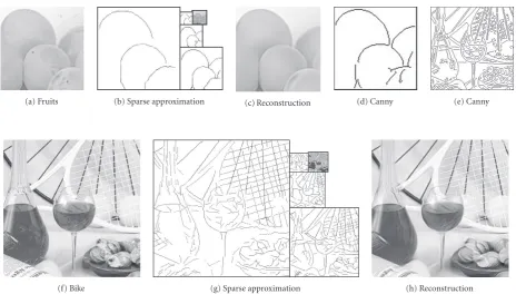
Figure7: Extraction of multiscale edges and reconstruction. (a) 96×96 pixels tile of the image “Fruits.” (f) 224×224 pixels tile of the image “Bike.” (b), (g) Edges extracted by the proposed model. The gray level indicates the amplitude of the edges given by the gain control mechanism. (c), (h) Reconstruction from edges. (d), (e) Edges extracted by Canny method.
Table2: Compression results in terms of PSNR for Lena, Boats, and Barbara.
Image bpp JPEG JPEG2K Our model
Lena 0.93 22.94 26.09 22.38
Boats 0.55 24.09 27.21 24.06
Barb 0.64 24.62 28.68 24.50
both in cases where few edges are selected (image compres-sion,Section 3.2) or when most of the edges are preserved (image denoising,Section 3.3).
3.2. Redundancy reduction
The sparse approximation and the chain coding are applied to several test images as summarized in Figures8,9,10, and
11andTable 2. Such experiments aim at evaluating the abil-ities of the model to reduce the redundancy of the visual in-formation. Redundancy reduction can be measured as the abilities of the model for image compression measured in terms compression rate (in bpp, bit per pixel), mathematical error, and perceptual quality (i.e., visual inspection). JPEG and JPEG-2000 are, respectively, the former and the actual golden standards in terms of image compression. They are then the principal methods to compare the model with. Ad-ditionally, a comparison with MP is included in Figures 9
and10.
The sparse approximation applied to a tile of “Lena” shown in Figure 8(a) induces the selection of a subdic-tionary shown inFigure 8(e). The chain coding compresses the image at 0.93 bpp and the reconstruction is shown in
Figure 8(d). The comparison at the same bit rate with both JPEG and JPEG-2000 compressed images are shown in Fig-ures8(b)-8(c). Other results at 1.03 and 0.56 bpp for the im-age “Bike” are shown in Figures9and10, where an additional comparison with MP is included.
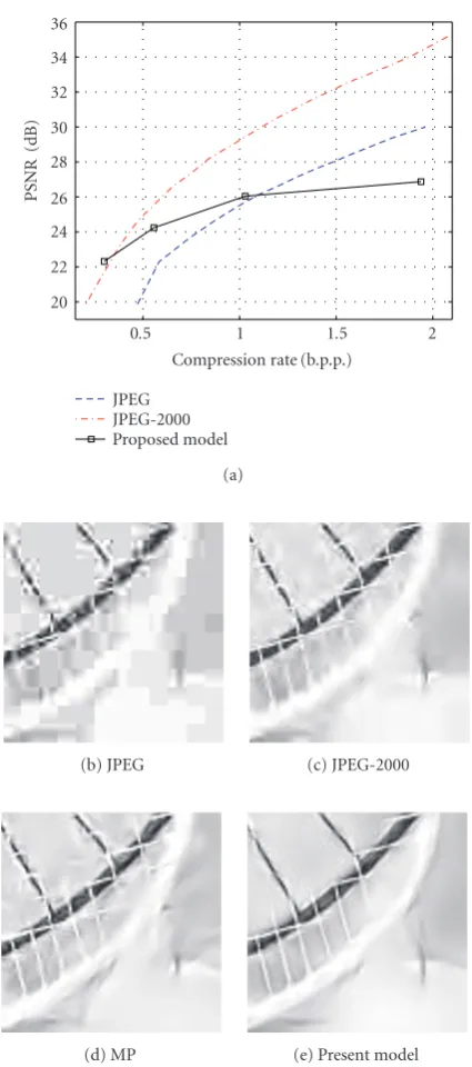
As shown inFigure 10(a)the compression standards pro-vide better results in terms of the peak-signal-to-noise ratio (PSNR)2at bit rates higher than 1 bpp for the image “Bike.”
In contrast at bit rates lower than 1 bpp, the current model provides better PSNR than JPEG, and at bit rates lower than 0.3 bpp better than JPEG-2000.
Nevertheless it is well known that mathematical errors are not a reliable estimation of the perceptual quality. Since images are almost exclusively used by humans, it is impor-tant to evaluate the perceptual quality by visual inspection. Moreover as the proposed scheme models the primary vi-sual areas, it is hoped that the distortions introduced present similarities with those produced by the visual system. Then one important expectation is that the distortions introduced
2The PSNR is measured in dB as PSNR= −20 log
(a) Original (b) JPEG
(c) JPEG-2000 (d) Present model
(e) Selected coefficients
Figure8: Compression of “Lena” at 0.93 bpp. (a) 64×64 original image. (b) In the JPEG-compressed image most of the contours and textures disappeared while block artifacts are salient. (c) Many de-tails of the JPEG-2000 image are smoothed, in particular the strips and hairs of the hat. Moreover artifacts appear specially on diagonal edges. (d) In the image compressed through sparse approximation, the disappearance of visual details does not yield high frequency ar-tifacts. (e) Selected subdictionary (here 2 every 3 coefficients have been zeroed along chains as proposed inSection 2.5).
by the model would appear less perceptible. This objective is important since a requirement of the lossy compression algo-rithms is the ability to introduce errors in a low perceptible manner.
A first remarkable property of the model is the lack of high-frequency artifacts. In contrast to JPEG or JPEG-2000, no ringing, aliasing, nor blocking effects appear. As a second good property, the continuity of contours appear particularly preserved. Finally, the gradients of luminance are
preserved smooth thanks to the elimination of isolated co-efficients. For those reasons, the reconstructed images tend to look natural even when the mathematical error is sig-nificantly higher. Compared with MP, the model provides a more structured arrangement of the selected coefficients (compareFigure 9(b)withFigure 9(c)), which induces more continuity of the contours in the reconstruction and reduces the appearance of isolated artifacts.
Reconstruction quality appears worst in junctions, cross-ings, and corners of the different scales (see alsoFigure 11(a)
for an image containing many of such features). This can be explained by the good adequacy of log-Gabor func-tions for matching edges and ridges and their worst match with junction and crossing features. One can argue that the present sparse approximation method should be completed by the implementation of junctions/crossing detectors as other models do [19]. Nevertheless this lies out of the scope of the present paper.
The second problem concerns textures which are gen-erally not well treated by edge extraction methods. One of the worst cases is the pure sinusoidal pattern which in some conditions does not even induce local-maxima in the modu-lus of complex log-Gabor functions. Nevertheless in the ma-jority of cases, textures can be considered as sums of edges. For example inFigure 8the bristles of Lena’s hat form a tex-ture and at least the most salient bristles are reproduced. In the same manner the texture constituted by the hat stria-tion is not reproduced integrally but the most salient stri-ations are preserved (note moreover that the stristri-ations also tend to disappear in the JPEG and JPEG-2000 compressed images). For further improving the reconstruction quality, and to extract more edges, a few additional passes of sparse approximation can be deployed. For example, a second pass allows the extraction of a significant part of the textures in Barbara’s scarf and in its chair as shown in Figure 11(h). Nevertheless the method does not allow to capture so much sparse approximations for textures than it does with con-tours. The compression quality at the same rate is then sig-nificantly lower. As future improvements, it could then be advantageous to deal with textures through a separate ded-icated mechanism exploiting the texture statistical regulari-ties as those proposed, for example, in [29,46], or more sim-ply using a standard wavelet coder as proposed in [28,30]. Such improvements stay nevertheless out of the scope of the present study.
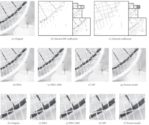
(a) Original (b) Selected MP coefficients (c) Selected coefficients
(d) JPEG (e) JPEG-2000 (f) MP (g) Present model
(h) Original (i) JPEG (j) JPEG-2000 (k) MP (l) Present model
Figure9: Compression results at 1.03 bpp. (a) 96×96 tile of the “Bike” image. (b) Coefficients selected by the MP algorithm. (c) Coefficients selected through the sparse approximation steps. (d) Compression with JPEG, PSNR=25.73 dB. (e) Compression with JPEG-2000, PSNR=
29.61 dB. (f) Reconstruction by the MP algorithm, PSNR=25.03 dB. (g) Compression by the proposed model, PSNR=26.05 dB. (h), (i), (j), (k), (l) 36×36 zoom tile for original, JPEG, JPEG-2000, MP, and the model, respectively.
3.3. Noise elimination
Denoising results are presented in Figures12,13, and14in comparison with the standard method by wavelet shrinkage [22] (orthogonal and undecimated wavelets “Db4” are used) and the GSM model using steerable pyramids [25]. For all methods the noise level is supposed to be known and the implementation proposed in [25] is used both for the GSM and the wavelet shrinkage methods. In denoising the qual-ity of reconstruction is important, then no edges should be missed in the sparse approximation. Consequently the sparse approximation steps are deployed two additional times on the reconstruction error, so as to extract the residual edges not detected in the first passes.
It is worth to note first that the method is able to tract and reconstruct almost all the image features. For ex-ample, the reconstruction of the image boats (Figure 12(e)) incorporates almost all the original image features. Neverthe-less some few edges are lost, for example, close to intricate junctions (see also Lena’s right eye and the upper part of the hat border inFigure 13(f)). Thus, at very low noise level the method cannot compete with other denoising methods due to that approximated reconstruction.
20 22 24 26 28 30 32 34 36
PSNR
(dB)
0.5 1 1.5 2
Compression rate (b.p.p.) JPEG
JPEG-2000 Proposed model
(a)
(b) JPEG (c) JPEG-2000
(d) MP (e) Present model
Figure 10: Compression results for the image Bike (original in
Figure 9). (a) Evolution of the PSNR for different compression rates. The proposed method can offer a reconstruction competitive with the compression standards at very high compression rates. (b), (c), (d), (e) Compression results at 0.56 bpp, respectively, for JPEG, JPEG-2000, MP, and the proposed model.
Lena a significant gain over the other methods (the difference is around 0.6 dB with GSM, seeFigure 14(a)). Figures14(b)–
14(f)show that contours are preserved sharper than in the other methods also at very high noise level.
Moreover as in the compression application, an impor-tant quality of the model is to yield reconstructions with-out high frequency artifacts. This allows in particular the
preservation of smooth gradients of luminance (see, e.g., Lena’s skin inFigure 13).
For explaining the results, it is worth noting that an im-portant difference between methods resides in the threshold-ing mechanism. Wavelet shrinkage only considers the ampli-tude of the coefficients, retaining the highest ones as signal and eliminating the smallest coefficients as noise. The GSM model considers the 3×3 neighborhood and the parent coef-ficient in the thresholding decision. In contrast the proposed model takes into account larger neighborhoods by consider-ing that contours are arranged in long chains of coaligned edges while noise is spatially incoherent.
4. CONCLUSIONS
We proposed a sparse approximation inspired from biologi-cal knowledge on V1 cortibiologi-cal cells and constructed following image processing criteria. It consists in a log-Gabor wavelet transform modeling V1 receptive fields followed by steps of thresholding, inhibition, facilitation and gain control mod-eling V1 nonlinearities and lateral interactions between cells. Those steps are able to extract continuous chains of coeffi-cients located on edges and ridges of the image, achieving an efficient contour extraction. Such procedure is incorporated in a sparse approximation scheme which selects uniquely those contour coefficients for building an approximation of the image. As an additional advantage of the method, the re-dundancy of sparse approximation can be further reduced by predictively encoding the chains of coefficients.
The redundancy reduction abilities allows the compres-sion of images preserving particularly the perceptual quality and approaching the results obtained by the standard image compression algorithms at high or very high compression rates. In parallel the ability for extracting contours shows promising results for image denoising since it preserves par-ticularly long lines and contours and at the same time it re-duces the appearance of artifacts. Best results are obtained at high noise levels.
Those encouraging results confirm the potential of over-complete transforms and sparse approximation algorithms for image processing and in particular for compression ap-plications. The present study shows that overcomplete trans-forms can offer important advantages in terms of perceptual quality in particular for avoiding the appearance of artifacts and preserving smooth gradients and continuous sharp con-tours. Another significant advantage is a high interpretabil-ity of transform coefficients in terms of edges and contours. It is remarkable also that the computational cost is reduced through the use of pure local operations and the nonitera-tive selection of the subdictionary. Moreover, the efficiency of the scheme for visual processing argues for the plausibility that similar processes could take place in the primary visual cortex.
(a) Boat (b) JPEG (c) JPEG-2000 (d) Present model
(e) Barbara (f) JPEG (g) JPEG-2000 (h) Present model
Figure11: Compression results of “Boats” at 0.55 bpp and of “Barbara” at 0.64 bpp. (a) This 96×96 tile of “Boats” image contains many junctions and corners, which are difficult features to be captured by the model. (b) Compression with JPEG. (c) Compression with JPEG-2000. (d) Compression using sparse approximation and chain coding. (e) 96×96 tile of “Barbara” image. This image contains textures which are also difficult features to be encoded by the model. (f) Compression with JPEG. (g) Compression with JPEG-2000. (h) Compression using the proposed model.
(a) Boats (b) Orthogonal wavelets (c) Undecimated wavelets
(d) GSM (e) Present model (f) Zoom
(a) Lena (b) Noisy version (c) Orthogonal wavelets
(d) Undecimated wavelets (e) GSM model (f) Present model
Figure13: Denoising results with Lena image at medium noise level. (a) 112×112 detail of the image “Lena.” (b) Same image corrupted by Gaussian noise for a PSNR of 20.22 dB. (c) After denoising using orthogonal wavelets a high level of artifacts appears. (d) The quantity and strength of artifacts is reduced thanks to the use of undecimated wavelets. (e) The GSM model allows an additional reduction of the number of artifacts. (f) The proposed model also allows to reduce the appearance of artifacts, preserving particularly smooth gradients of luminance. Nevertheless the model shows difficulties in capturing some intricate features in particular close to junctions (see, e.g., the right eye) and to adjacent parallel lines (e.g., upper end of the hat border).
0 2 4 6 8 10
Gain
(dB)
33.90 26.02 20.22 14.92 11.97 9.21 6.88 Noise level (PSNR dB)
Sparse log-Gabor wavelets Steerable pyramid & GSM model Undecimated wavelet shrinkage Orthogonal wavelet shrinkage
(a) Evolution with noise level
(b) Orthogonal (c) Undecimated (d) GSM
(e) Model (f) Noisy
separated texture representation as already proposed by sev-eral authors. Many improvements are also possible in all the different steps of the algorithm, in particular to im-prove the selection of coefficients by incorporating a statis-tical framework linking the different saliency measurements (chain length, presence of parent coefficients, and coefficient amplitude), or for further exploiting the predictability of the coefficients across scales for image compression.
ACKNOWLEDGMENTS
Thanks to Laura Rebollo-Neira, Sandrine Anthoine, and Nader Yeganefar for discussions on the mathematical as-pects of sparse approximation. This work has been supported in part by the grants TEC2004-00834, PI040765, TEC2005-24046-E, and TEC2005-24739-E. SF, RR and LP are sup-ported by grants from MEC-FPU, CSIC-I3P and EC IP project FP6-015879,” “FACETS,” respectively.
REFERENCES
[1] E. P. Simoncelli, W. T. Freeman, E. H. Adelson, and D. J. Heeger, “Shiftable multiscale transforms,”IEEE Transactions on Information Theory, vol. 38, no. 2, pp. 587–607, 1992. [2] M. N. Do and M. Vetterli, “The contourlet transform: an effi
-cient directional multiresolution image representation,”IEEE Transactions on Image Processing, vol. 14, no. 12, pp. 2091– 2106, 2005.
[3] N. Kingsbury, “Complex wavelets for shift invariant analysis and filtering of signals,”Applied and Computational Harmonic Analysis, vol. 10, no. 3, pp. 234–253, 2001.
[4] D. L. Donoho and A. G. Flesia, “Can recent innovations in har-monic analysis ‘explain’ key findings in natural image statis-tics?”Network: Computation in Neural Systems, vol. 12, no. 3, pp. 371–393, 2001.
[5] S. G. Mallat and Z. Zhang, “Matching pursuits with time-frequency dictionaries,”IEEE Transactions on Signal Process-ing, vol. 41, no. 12, pp. 3397–3415, 1993.
[6] S. S. Chen, D. L. Donoho, and M. A. Saunders, “Atomic de-composition by basis pursuit,”SIAM Journal of Scientific Com-puting, vol. 20, no. 1, pp. 33–61, 1998.
[7] L. Perrinet, M. Samuelides, and S. Thorpe, “Coding static nat-ural images using spiking event times: do neurons cooperate?”
IEEE Transactions on Neural Networks, vol. 15, no. 5, pp. 1164– 1175, 2004.
[8] S. Fischer, G. Crist ´obal, and R. Redondo, “Sparse overcom-plete Gabor wavelet representation based on local competi-tions,”IEEE Transactions on Image Processing, vol. 15, no. 2, pp. 265–272, 2006.
[9] A. E. C. Pece, “The problem of sparse image coding,”Journal of Mathematical Imaging and Vision, vol. 17, no. 2, pp. 89–108, 2002.
[10] L. Perrinet, “Feature detection using spikes: the greedy ap-proach,”Journal of Physiology Paris, vol. 98, no. 4–6, pp. 530– 539, 2004.
[11] J. G. Daugman, “Uncertainty relation for resolution in space, spatial frequency, and orientation optimized by two-dimensional visual cortical filters,”Journal of the Optical So-ciety of America. A, Optics and Image Science, vol. 2, no. 7, pp. 1160–1169, 1985.
[12] R. L. De Valois, D. G. Albrecht, and L. G. Thorell, “Spatial fre-quency selectivity of cells in macaque visual cortex,”Vision Re-search, vol. 22, no. 5, pp. 545–559, 1982.
[13] B. A. Olshausen and D. J. Field, “Sparse coding with an over-complete basis set: a strategy employed by V1?”Vision Re-search, vol. 37, no. 23, pp. 3311–3325, 1997.
[14] M. K. Kapadia, G. Westheimer, and C. D. Gilbert, “Spatial dis-tribution of contextual interactions in primary visual cortex and in visual perception,”Journal of Neurophysiology, vol. 84, no. 4, pp. 2048–2062, 2000.
[15] S. Mandon and A. K. Kreiter, “Rapid contour integration in macaque monkeys,”Vision Research, vol. 45, no. 3, pp. 291– 300, 2005.
[16] R. F. Hess, A. Hayes, and D. J. Field, “Contour integration and cortical processing,”Journal of Physiology Paris, vol. 97, no. 2-3, pp. 105–119, 2003.
[17] S. Grossberg, E. Mingolla, and J. Williamson, “Synthetic aper-ture radar processing by a multiple scale neural system for boundary and surface representation,”Neural Networks, vol. 8, no. 7-8, pp. 1005–1028, 1995.
[18] T. Hansen, W. Sepp, and H. Neumann, “Recurrent long-range interactions in early vision,” inEmergent Neural Com-putational Architectures Based on Neuroscience, S. Wermter, J. Austin, and D. Willshaw, Eds., vol. 2036 ofLNAI, pp. 127–138, Springer, Heidelberg, Germany, 2001.
[19] F. Heitger, L. Rosenthaler, R. Von der Heydt, E. Peterhans, and O. Kubler, “Simulation of neutral contour mechanisms: from simple to end-stopped cells,”Vision Research, vol. 32, no. 5, pp. 963–981, 1992.
[20] S.-C. Yen and L. H. Finkel, “Extraction of perceptually salient contours by striate cortical networks,”Vision Research, vol. 38, no. 5, pp. 719–741, 1998.
[21] R. VanRullen, A. Delorme, and S. J. Thorpe, “Feed-forward contour integration in primary visual cortex based on asyn-chronous spike propagation,” Neurocomputing, vol. 38–40, no. 1–4, pp. 1003–1009, 2001.
[22] R. R. Coifman and D. Donoho, “Translation-invariant de-noising,” inWavelets and Statistics, A. Antoniadis and G. Op-penheim, Eds., vol. 103 ofLecture Notes in Statistics, pp. 125– 150, Springer, New York, NY, USA, 1995.
[23] S. Fischer, F. Sroubek, L. Perrinet, R. Redondo, and G. Crist ´obal, “Self-invertible 2D log-Gabor wavelets,” Interna-tional Journal of Computer Vision, to appear.
[24] S. Fischer, R. Redondo, L. Perrinet, and G. Crist ´obal, “Sparse Gabor wavelets by local operations,” in Bioengineered and Bioinspired Systems II, R. A. Carmona, Ed., vol. 5839 of Pro-ceedings of SPIE, pp. 75–86, Sevilla, Spain, May 2005. [25] J. Portilla, V. Strela, M. J. Wainwright, and E. P.
Simon-celli, “Image denoising using scale mixtures of Gaussians in the wavelet domain,”IEEE Transactions on Image Processing, vol. 12, no. 11, pp. 1338–1351, 2003.
[26] S. Mallat and S. Zhong, “Characterization of signals from mul-tiscale edges,”IEEE Transactions on Pattern Analysis and Ma-chine Intelligence, vol. 14, no. 7, pp. 710–732, 1992.
[27] J. H. Elder, “Are edges incomplete?”International Journal of Computer Vision, vol. 34, no. 2-3, pp. 97–122, 1999.
[29] J.-L. Starck, M. Elad, and D. L. Donoho, “Image decompo-sition via the combination of sparse representations and a variational approach,”IEEE Transactions on Image Processing, vol. 14, no. 10, pp. 1570–1582, 2005.
[30] M. Wakin, J. Romberg, H. Choi, and R. Baraniuk, “Image compression using an efficient edge cartoon + texture model,” inProceedings of Data Compression Conference (DCC ’02), pp. 43–52, Snowbird, Utah, USA, April 2002.
[31] J. Canny, “Computational approach to edge detection,”IEEE Transactions on Pattern Analysis and Machine Intelligence, vol. 8, no. 6, pp. 679–698, 1986.
[32] M. C. Morrone and D. C. Burr, “Feature detection in human vision: a phase-dependent energy model,”Proceedings of the Royal Society of London. Series B. Biological Sciences, vol. 235, no. 1280, pp. 221–245, 1988.
[33] B. W. Rust and H. E. Rushmeier, “A new representation of the contrast sensitivity function for human vision,” inProceedings of the International Conference on Imaging Science, Systems, and Technology (CISST ’97), H. R. Arabnia, Ed., pp. 1–15, Las Vegas, Nev, USA, June 1997.
[34] J. J. Atick, “Could information theory provide an ecological theory of sensory processing?”Network: Computation in Neu-ral Systems, vol. 3, no. 2, pp. 213–251, 1992.
[35] S. G. Chang, B. Yu, and M. Vetterli, “Adaptive wavelet thresh-olding for image denoising and compression,”IEEE Transac-tions on Image Processing, vol. 9, no. 9, pp. 1532–1546, 2000. [36] W. H. Bosking, Y. Zhang, B. Schofield, and D. Fitzpatrick,
“Orientation selectivity and the arrangement of horizontal connections in tree shrew striate cortex,” Journal of Neuro-science, vol. 17, no. 6, pp. 2112–2127, 1997.
[37] N. Kr¨uger, “Collinearity and parallelism are statistically signif-icant second-order relations of complex cell responses,”Neural Processing Letters, vol. 8, no. 2, pp. 117–129, 1998.
[38] W. S. Geisler, J. S. Perry, B. J. Super, and D. P. Gallogly, “Edge co-occurrence in natural images predicts contour grouping performance,”Vision Research, vol. 41, no. 6, pp. 711–724, 2001.
[39] P. Kovesi, “Phase congruency detects corners and edges,” in
Proceedings of the 7th International Conference on Digital Image Computing: Techniques and Applications (DICTA ’03), pp. 309– 318, Sydney, NSW, Australia, December 2003.
[40] D. Hubel,Eye, Brain, and Vision, Scientific American Library Series, W. H. Freeman, New York, NY, USA, 1988.
[41] A. Dobbins, S. W. Zucker, and M. S. Cynader, “Endstopping and curvature,”Vision Research, vol. 29, no. 10, pp. 1371–1387, 1989.
[42] A. Pasupathy and C. E. Connor, “Population coding of shape in area V4,”Nature Neuroscience, vol. 5, no. 12, pp. 1332–1338, 2002.
[43] R. Redondo and G. Crist ´obal, “Lossless chain coder for gray edge images,” inProceedings of IEEE International Conference on Image Processing (ICIP ’03), vol. 2, pp. 201–204, Barcelona, Spain, September 2003.
[44] H. Freeman, “On the encoding of arbitrary geometric configu-rations,”IRE Transactions on Electronic Computers, vol. 10, pp. 260–268, 1961.
[45] G. P. Howard, “The design and analysis of efficient lossless data compression systems,” Tech. Rep. CS-93-28, Department of Computer Science, Brown University, Providence, RI, USA, 1993.
[46] J. Portilla and E. P. Simoncelli, “A parametric texture model based on joint statistics of complex wavelet coefficients,”
Inter-national Journal of Computer Vision, vol. 40, no. 1, pp. 49–70, 2000.
[47] S. Fischer,New contributions in overcomplete image represen-tations inspired from the functional architecture of the primary visual cortex, Ph.D. thesis, Technical University Madrid High Technical School of Telecommunication Engineering, Depart-ment of Electronic Engineering, Spain, 2007.
Sylvain Fischer received the M.S. degree in telecommunication engineering from ENST, Telecom Paris, France and ETSIT-UPM, Madrid, Spain in 2000. He is finish-ing the Ph.D. in the Instituto de ´Optica, CSIC, Madrid. His current research inter-ests include vision modeling and sparse ap-proximation.
Rafael Redondoreceived in 2002 his En-gineering degree from ETSIT (Universidad Polit´ecnica de Madrid, Spain) focused on developing new image compression meth-ods based on vision models. He currently works as an Ph.D. student at Instituto de
´
Optica (CSIC) since 2001. Among his re-search fields are vision modeling, image and volumetric coding algorithms and time-frequency representations applied to pat-tern recognition, image fusion and compression.
Laurent Perrinet received an Engineer-ing degree from SUPAERO, in Toulouse (France) with a focus on signal and im-age processing using artificial neural net-works and a Ph.D. degree in computational neuroscience. He is currently a Researcher at INCM-CNRS in Marseille (France). His research interests focus on bridging lower-level neural computations with functional models of inference and spatio-temporal
in-tegration aiming at understanding low- to mid-level visual percep-tion.