Volume 2011, Article ID 183547,13pages doi:10.1155/2011/183547
Research Article
A Self-Adaptive Approach for the Detection
and Correction of Stripes in the Sinogram:
Suppression of Ring Artifacts in CT Imaging
A. N. M. Ashrafuzzaman,
1Soo Yeol Lee,
2and Md. Kamrul Hasan
1, 21Department of Electrical and Electronic Engineering, Bangladesh University of Engineering and Technology, Dhaka 1000, Bangladesh 2Department of Biomedical Engineering, Kyung Hee University, Kyungki 446-701, Republic of Korea
Correspondence should be addressed to Md. Kamrul Hasan,[email protected]
Received 4 June 2010; Revised 2 August 2010; Accepted 14 August 2010
Academic Editor: Antonio Napolitano
Copyright © 2011 A. N. M. Ashrafuzzaman et al. This is an open access article distributed under the Creative Commons Attribution License, which permits unrestricted use, distribution, and reproduction in any medium, provided the original work is properly cited.
The digital X-ray detectors often generate stripe artifact in the sinogram which in turn creates ring artifact in the reconstructed micro-Computed Tomography (μ-CT), C-Arm CT, and most recent dental CT images. Such ring artifacts not only obscure image details in the regions of interest but also mask the whole image with some artifacts. In this paper, novel techniques are proposed for the detection and suppression of ring artifacts in the sinogram domain. As ring artifacts are manifested as edge creating stripes, single or contiguous, in the sinogram, they are detected based on a set of specific conditions derived from the second derivative of the sinogram and a new self-adaptive threshold computed from its first derivative. A new method for the detection of wide band contiguous stripes using the mean curve and multilevel polyphase decomposition of the given sinogram is also proposed here. For the correction of ring artifacts, novel variable window moving average (VWMA) and weighted moving average (WMA) filters are proposed in this work. To evaluate and compare the performance of the proposed algorithm, various types of synthetic and real
μ-CT images are used. Experimental results show that the proposed method can detect ring artifacts with high accuracy and thus remove them more effectively without imparting noticeable distortion in the image as compared to other reported techniques.
1. Introduction
Computed tomography (CT) is an imaging technique capa-ble of generating high-resolution three-dimensional (3D) images of an object from two-dimensional (2D) X-ray projection data or 2D slices from 1D projection data [1,2]. Currently, CT devices are widely used to evaluate bone specimens [3], for analysis of coronary artery walls and cancer research [4]. It is also used to screen genetically engineered small animals to investigate new drugs or therapy [5]. Nonmedical researchers have applied this technology to nondestructive testing. Modern high resolution CT machines are nowadays equipped with digital X-ray detectors (e.g., CMOS flat-panel detectors (CMOS-FPDs), or CCDs) which often create ring artifacts in the reconstructed CT images because of defective and/or miscalibrated detector elements, and dusty or damaged scintillator screens. These
artifacts appear in μ-CT, C-Arm CT, and modern dental CT images in the form of a circle, centered at the center of rotation of the system. They severely impair visualization and quantification of anatomic and pathological features in the regions of interest. Therefore, removal or at least significant reduction of these artifacts is essential.
to remove ring artifacts from the CT images taken with the FPDs. Though detector calibration schemes and built-in white and dark image correction algorithms can reduce the detector pixel problem to some extent, the ring artifact problem cannot be avoided in the 2D radiographic projec-tion data. Even a small imperfecprojec-tion produces ring artifact in the reconstructed image. Ring correction algorithm as a postprocessor is, therefore, indispensable while using the digital X-ray detectors.
Several methods have been reported so far to suppress the ring artifacts in CT images [6–16]. Ring artifact reduc-tion without impairing image quality is still a challenging problem for the researchers. Directly processing the ring artifact corrupted image as reported in [6–8] is one way which may be referred to as the postprocessing approaches. While it may be tempting to detect and remove the artifact in the image domain rather than the sinogram domain, the extra artifacts inherently generated along with the ring artifacts due to the filtered back projection reconstruction procedure cannot be easily detected and removed by a signal processing technique in the image domain. Since it is the 2D radiographic projection data, generally known as the sinogram [1], which are actually corrupted, some reported methods dealt with the raw sinogram, referred to as the preprocessing approaches [10–16]. At early stages, flat-field method was proposed in the literature [10]. This involved multitime scanning through air prior to main scanning of the object. Though the destruction of useful information was checked in this method, expected amount of ring reduction was not achieved [6]. Later on, a sinogram correction technique using the original corrupted mean curve and its smoothed version has been proposed in [11]. The moving average (MA) filter is used to smooth the mean curve as it is simple and efficient. However, the selection of the window size is very crucial while using this method. A large window may result in the blurring effect while a small window results in weak filtering. Moreover, the correction technique in [11,12] is not effective for the compensation of varying intensity sharp rings. As the median is better than the mean at preserving the sharp details due to image feature, the median filtering (MedF) method has been also used by the researchers [12–14]. The median filter is particularly good in removing sharp noise such as, shot noise or “salt and pepper” noise, while preserving the edges. Thus the MedF may be suitable for the reduction of isolated rings but not for the clustered rings. The 2D wavelet-based method presented in [13] has been designed to eliminate ring artifacts from a cone beam CT image. As this technique is particularly applicable to cone beam geometry, it requires modification to implement and investigate its performance for fan or parallel beam geometry. In [15], a frequency domain filtering technique has been reported for the removal of ring artifacts. The basic concept was to use a low-pass filter to suppress the high frequency components resulted from the ring artifacts. The filter cut-offfrequency and order have to be selected appropriately depending on the type and number of defects in the raw projection data. Very recently a wavelet-Fourier filter has been reported in [16] for the correction of stripes in the sinogram. The performance of this method,
however, significantly degrades when an image is particularly corrupted by a sharp ring of varying intensity.
In this paper, we propose novel self-adaptive approaches for the detection and correction of stripes in the sinogram with a view to suppress ring artifacts in CT imaging. As it is crucially important to detect stripes (both isolated and contiguous) for the distortionless processing of the sinogram data, we propose here a highly accurate method for the detection of stripe artifacts in the sinogram responsible for ring artifacts in the reconstructed image. Only the detected stripes are then corrected using the new adaptive moving average filters proposed in this work. The stripes causing edges in the sinogram are detected based on derivative property of the windowed sinogram, self-adaptive threshold, mean-curve, and multilevel-polyphase decomposition con-cept. To overcome the limitations of the conventional moving average- (MA-) based schemes, the new variable window moving average (VWMA) and weighted moving average (WMA) filters proposed in this work are used appropriately to correct both the isolated and contiguous stripes. The elegance of the proposed iterative method is that it rarely distorts any good pixel and the correction is only made where the detection algorithm finds a fault.
The paper is organized as follows. Section 2 describes the proposed new methods for the detection and correction of stripes in the sinogram. The experimental results are presented in Section 3. Finally, the paper concludes with some remarks inSection 4.
2. Ring Suppression Method
In this work, we view the ring artifact removal problem as equivalent to stripe error correction of the sinogram data. Unlike the conventional approaches where the ring generating artifact is removed from the sinogram using a normalization technique [12], we propose here a new stripe detection and correction scheme that detects the stripe generating detector elements first and then corrects their responses for all angle of view dynamically based on the degree of corruption. The proposed method therefore, consists of two parts: stripe detection and stripe correction.
2.1. Stripe Detection. The isolated ring artifact in the recon-structed image is due to a stripe artifact in P(θ,n) for all viewsθ. These stripes create discontinuity in the projection image. The first derivative of the data characterizes these positions by showing relatively larger values as compared to their neighborhood. Therefore, the sum of the first derivatives, for allθ, will show two consecutive larger spikes of opposite polarity in a row around a detector if it creates a stripe. To identify such transition points, the derivative of this sum of the first derivative will be more useful since it will give a much larger value than its neighborhood at these points. To make a decision if a detector creates a stripe, a measure of this second derivative is compared with a threshold calculated from the responses of the neighboring detector elements.
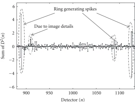
is because a threshold determined from the whole sinogram is not effective in identifying only stripes from the rest of the detector responses. As depicted in Figure 1, a global threshold will either fail to detect all stripes or will include false positive due to large spikes from the image details. The sinogramP(θ,n) is, therefore, divided into overlapping framesPk(θ,n) of size (nv×ndf), wherenvis the total number of views,ndf is the frame width (<nd, the total number of detectors), and the subscriptk refers to thekth frame with
nk being the center of the frame. We choosendf = 9 and the displacement between the two successive frames as one pixel width across the detectors. To make the frame image independent, we normalize each frame to bring the data in the range [0,1]. Now, the first and second derivatives of the normalized framePk(θ,n) can be calculated as
Dz k(θ,n)=
z
l=0 (−1)la
zlPk(θ,n−l), (1)
wherezdenotes the order of the derivative and
azl= ⎧ ⎨ ⎩
1, ifl=0,z;
z, otherwise. (2)
The sum of the derivative, for z = 1, 2, of the kth frame of the corrupted sinogram and an appropriately determined threshold fromD1
k(θ,n) will be utilized to identify the stripe creating positions. The sum is given by
Dzk(n)=
θ Dz
k(θ,n), z=1, 2,n=1, 2. . . n f d. (3)
Now, to ascertain if thenkth position of the frame contains a stripe, we check the following three conditions if
(1)|D2k(nk+ 1)|>|D 2 k(nk)|,
(2)|D2k(nk+ 1)|>|D2k(nk+ 2)|,
(3)|D2k(nk+ 1)| ≥Tk,
where Tk is the threshold determined from the responses of the detector elements of the kth frame. If the above conditions are jointly satisfied, then the nkth position of thekth frame contains a ring generating stripe. Shifting the frame by one detector position in each step, all the isolated stripes can be detected.
The question now is how we can determine a self-adaptive threshold (Tk) that can adapt itself with the variation of the sinogram contents. It may be necessary that the sum of the second derivative be compared with a very small threshold to isolate the spike related to a stripe in the sinogram for a particular detector. In another occasion, to identify a stripe a larger threshold value may be required because of the change in image information. In Figure 1, such 4 places are shown where the spikes are located. We see that, among the ring generating spikes, one of them (3rd ellipse from the left) is relatively smaller than the spike due to the image details (2nd ellipse from the left). To isolate
900 950 1000 1050 1100
−6
−4
−2 0 2 4
6 Ring generating spikes
Due to image details
Su
m
o
f
D
2(n
)
Detector (n)
Figure1: A cropped view of the sum of the second derivative of the
whole sinogram (P(θ,n)) versus detector position—explaining the necessity of a local threshold instead of a global one.
the third one, any global threshold will detect some of the good detectors as faulty detectors. Therefore, the concept of a global threshold is not suitable for the underlying problem of discriminating a faulty detector from a good one. Instead, we can take the neighborhood’s difference information (D1
k(θ,n)) of a certain detector to formulate a local and frame-based threshold.
If the center detector of the kth frame, nk, causes a stripe, then in the first derivative (D1
k(θ,n)) of the detector responses, nk and nk + 1 positions will contain error. Therefore, to determine a threshold we construct a subframe excluding the erroneous lines fromD1
k(θ,n). We also exclude nk−1 line for symmetry consideration. The modified frame or the subframe is then given by
D1
ks(θ,t)=D1ks(θ,n)n /=nk,n /=nk±1, t⊂n. (4)
Ideally, when a subframe is very homogeneous, one can define a threshold using the mean of|D1
ks(θ,t)|. But from practical considerations, we propose to use the mean of the absolute value of the dominant polarity group of D1
ks(θ,t) instead. Two quantities α+
ks(j) and α−ks(j) representing the positive and negative values in the first derivative,D1
ks(θ,t), respectively, can be calculated as
α+ks
j =. D1ks(θ,t)>0, j⊂[0, (nv×t)]. (5)
α−ksj =. D1
ks(θ,t)<0, j⊂[0, (nv×t)]. (6)
For the regions from where the image information just starts (e.g., the first and last few detectors) in the sinogram and where a faulty detector is present in the neighborhood region
(Figure 2(c)), the absolute mean as well as the population of
50 100 150 200 250 300 350 400 450 Vi ew | D
2 (nk
) | 0 20 40 60 80 100 120 140
Detector (n) 311 313 315 317 319
Detector (n) 311 313 315 317 319
Tk
(i) (ii)
(a)
|
D
2 (nk
) | 50 100 150 200 250 300 350 400 450 Vi ew 0 20 40 60 80 100 120 140
Detector (n) 312 314 316 318 320
Detector (n) 312 314 316 318 320
Tk
(i) (ii)
(b)
Detector (n)
|
D
2 (nk
)
|
Tk
680 682 684 686 688
Detector (n) 680 682 684 686 688 50 100 150 200 250 300 350 400 0 50 100 150 200 250 300 350 400 450 Vi ew (i) (ii) (c) | D
2 (nk
) | 50 100 150 200 250 300 350 400 450 Vi ew 0 2 4 6 8 10 12 14
935 937 939 942 943
Detector (n) 935 937 939 942 943
Detector (n)
Tk
(i) (ii)
(d)
|
D
2 (nk
)
|
Tk
Detector (n) 50 100 150 200 250 300 350 400 450 Vi ew 0 0.5 1 1.5 2 2.5 3 3.5 4 4.5
1009 1011 1013 1015 1017
Detector (n) 1009 1011 1013 1015 1017
(i) (ii)
(e)
|
D
2 (nk
) | 50 100 150 200 250 300 350 400 450 Vi ew 0 20 40 60 80 100 120 140 160
Detector (n) 884 886 888 890 892
Detector (n) 884 886 888 890 892
Tk
(i) (ii)
(f)
Figure2: Examples of stripe detection using sinogram frames. a(i)–f(i) show some typical frames of a CT sinogram and (a)(ii)–(f)(ii) show
|D2k(n)|and the corresponding thresholdTk(dotted line). Dynamic nature ofTkis evident. (a) Moderate stripe at the center. (b) No stripe
at the center but one just before it. (c) Moderate stripe at the center but a very strong stripe in the neighborhood. (e) Very weak stripe at the center. (e) No stripe in the frame.|D2k(n)|may be misleading but the dynamic threshold confirms no stripe here. (f) Three consecutive
stripes (887–889) whereTkis unexpectedly low and|D2k(n)|are misleading.•shows the point of interest in each figure.
computation, the following statements are used to modify the two quantities in (5) and (6):
α+ks j . = ⎧ ⎪ ⎨ ⎪ ⎩
α+ks
j if α+ks> std
α+ks j , α+ ks j α+
ks(j)<δ×std(α+ks(j))
, otherwise.
α−ks j . = ⎧ ⎪ ⎪ ⎨ ⎪ ⎪ ⎩
α−ks
j ifα−ks>std
α−ks
j ,
α−ksj
|α−ks(j)|<δ×|std(α−ks(j))|
, otherwise,
where α−ks and α+ks are the mean of |α−ks(j)| and α+ks(j), respectively, andδis a constant. The ratio of the number of elements in the dominant class of polarity inD1ks(θ,t) to that in the subframe is denoted byβkand is given by
βk=
maxLα+ ks
j ,Lα−ks
j Lα+
ks
j +Lα−ks
j , (8)
whereL(·) is the length of the argument. What portion of the subframe is occupied by the dominant class of polarity is indicated by βk. In this work, the dynamic threshold is calculated as
Tk=γ×αks+/−×βk×nv, (9)
where α+/−
ks indicates the mean of either α+ks(j) or |α−ks(j)| and is denoted by either α+
ks or αks−. The multiplication of βk by the total number of views nv gives on average the population of the dominant class of polarity in a detector position for allθ. The constant γ = 2 is chosen, because a parameter computed from the first derivative is used to define this threshold but it is compared with the sum of the second derivative which has essentially the double magnitude in an edge. The threshold as defined above is expected to vary according to the neighborhood information content and hence it will, in general, be different for every frame.
The insight of the stripe detection algorithm developed here and the performance of the self-adaptive threshold can be better understood from the examples presented in
Figure 2. This figure explicitly shows the value of the dynamic
threshold obtained for different characteristic sinogram frames along with |D2k(n)|. Therefore, all the three stripe determining criteria can be checked from this figure. The arbitrarily selected frames contain strong, moderate, weak, and very weak stripes at the center along with stripes at the neighborhood. Frames containing no stripes are also considered. In all the cases of Figures 2(a)–2(e)except for
Figure 2(f), the proposed algorithm successfully detects if
there is any ring generating stripe at the center of the frame. It is to be noted that the stripe detecting threshold is varying widely even in these few selections. This justifies that a thumb rule-based threshold or a global threshold cannot be even a reasonable choice.
The new stripe detection algorithm presented above is derived based on an assumption that when the center position,nk, of thekth frame contains a stripe, there exits no stripe adjacent to it. If this is violated, for example,
Figure 2(f), then all the stripes in successive frames may not
be detected by the algorithm. To enable detection of the contiguous stripes, we propose here a combined technique using the mean curve and polyphase decomposition of the original corrupted sinogram.
The mean curveP(n) ofP(θ,n) can be obtained as
P(n)= 1
N
θ
P(θ,n). (10)
The mean curveP(n) is normalized to make its magnitude range image independent and also to make the threshold
determining constraint global. It is to be noted that the con-tiguous stripes in the mean curve create wide peak/trough. By smoothing this mean curve, that is, removing the high frequency components, we can use it to locate them. We use the moving average method to smooth the mean curve as
Ps(n)= 1 2S+ 1
S
m=−S
P(n−m), (11)
where Ps(n) is the smoothed version of P(n) and Sis the span factor. The difference betweenP(n) andPs(n) is called difference curve and is denoted asPd(n). Larger span factor oversmoothes the mean curve and creates some false band in the difference curve, where smaller span factor treats wide peak/trough as an image detail and therefore cannot differentiate the bands. To minimize both effects, we choose
S =2 as a span factor. Then by choosing a thresholdη, we can detect the wide peaks/troughs from the difference curve. The set of the detector elements which satisfies the condition,
Pd(n) > η, is treated as the band ring creating elements and is denoted by Bm. Here, η is an image-dependent threshold and is observed to vary in the range of 0.005∼ 0.006. FromFigure 3(a), we observe that, the best possible width represented by the smooth mean curve is not the actual width of the trough. Moreover, there are three possible bands (peaks/troughs) in the difference curve as shown in
Figure 3(b). Therefore, some false positive may be included
inBm depending on the threshold chosen. ThusBm is not fully reliable for bandwidth determination and truly ring creating band identification.
To resolve the ambiguities inBm, we propose here a new idea using the polyphase decomposition of the sinogram:
PMq(θ,n)=P
θ,nM+q−1 ,
0≤n≤nd−1, 1≤q≤M,
(12)
where PMq(θ,n) is the qth polyphase component of the M level decomposition ofP(θ,n). Since all the contiguous stripes can be considered to be isolated stripes in these polyphase components, the previous isolated stripe detection algorithm can be used for these subsequences. A sinogram may contain contiguous stripes of different bandwidths. Lower level decomposition is effective for smaller bands and higher level decomposition is effective for wider bands. Therefore, we take the advantage of multilevel polyphase decomposition. Finally, a string namedBsof unique stripe generating detector positions is formed from the outcomes of the single stripe detection algorithm applied toPMq(θ,n), M = 2,. . .,Mmax, 1 ≤ q ≤ M. But edges between the background and object of the original sinogram may create stronger edges in the polyphase components. They create large values in second derivative and hence may also be detected. Therefore,Bsrepresents a group of stripes of which all may not be truly corrupted contiguous stripes. But inBs, the ranges of the truly corrupted contiguous stripes represent the actual widths.
875 880 885 890 895 900 3.82
3.84 3.86 3.88 3.9 3.92 3.94 3.96 3.98
Detector position
M
ean
val
u
e
Detected range from the difference
curve 1Ps(n)
1P(n)
Actual range
(a)
−0.03 −0.02 −0.01 0 0.01 0.02
Di
ff
er
enc
e
1Pd(n)
875 880 885 890 895 900
Detector position
(b)
Figure3: Detection of contiguous stripes using the mean curve. (a) A cropped mean curve and its smoothed version. (b) Difference curve.
represents the common set of detectors of Bm andBs and we consider them as truly band ring generating detectors. Then for every value of the setB, the corresponding range of the contiguous stripes is determined fromBs. Finally, the unique stripe positions for both the single (as determined for
M =1 in the previous stage) and contiguous stripes are the total corrupted locations in the sinogram.
2.2. Stripe Correction. The error-free response of stripe generating detector elements can be estimated using its neighborhood information. In this work, we propose new 1D dynamic moving average filters for the estimation of the defective pixel response. The filter corrects the defective pixels for each view one by one iteratively. The responses of the good detectors are not changed and thus the process is called distortionless. New variable window moving average (VWMA) and weighted moving average (WMA) filters are formulated here to make a correction. The VWMA and WMA have relative advantages and we exploit the merits of both to remove artifacts. For each view n, every faulty detector element is corrected iteratively according to the value of an index called “central difference”. The windowed central difference ofP(θv,n), whereP(θv,n) is the 1D slice of the sinogram along the viewnv, is calculated as
ΔP(θv,n)
= 1 2Ln
Ln
k=1
2P(θv,n)−P(θv,n−k)−P(θv,n+k)n=n,
(13)
where | · | denotes the absolute value. Here, the central difference is calculated at the corrupted locations (n) only. The window span factor (Ln) indicates how many adjacent detectors in a particular view are to be taken. To correct
a defective pixel instead of taking just two adjacent pixels, we consider more pixels depending on the degree of error or the extent of deviation for making a better correction. A weak fault can be corrected using the adjacent 2–4 pixels but a strong fault needs more neighborhood information. Therefore, the concept of variable window MA is expected to be useful. However, too large a window size according to the degree of deviation is not a good choice for correction since too further pixels information will be involved then. Instead, we keep the window size small even for the strongly deviated pixels but attach some weights to the moving average, that is, give a faulty location the least weight (we use zero weight, that is, no information will be taken from the defective pixel) and the neighborhood pixels in a particular view relatively larger weights. Such a scheme will eliminate the blurring effect as observed in the conventional MA filters. A factor deciding about the extent of smoothing can be chosen to be proportional to the windowed central difference. A parameterλnis calculated as
λn=K×ΔP(θv,n), (14)
whereKis a proportionality constant and our experiments suggest that it may be chosen to beK=220. This parameter is selected so as to give a larger value ofλn, where significant deviations are found. A weighting function is to be defined to meet the requirement stated above. Here, an exponential weight function is chosen for that purpose:
w(n)= ⎧ ⎪ ⎨ ⎪ ⎩
(λn)−|n−n| ifn /=n,
0, otherwise. (15)
window WMA filter as defined by (17). But in places where the degree of deviation is not so high, the VWMA is used. Thus forλn≤1, we use the VWMA as described by (17) and setλn=1 to attach uniform weight to the VWMA. The span factorLnfor making the correction is chosen according to the central difference because the magnitude of ΔP(nv,n)|n=n indicates the degree of corruption:
Ln= ⎧ ⎪ ⎨ ⎪ ⎩
Lf ifλn>1,
roundJ×ΔP(θv,n)
ifλn≤1,
(16)
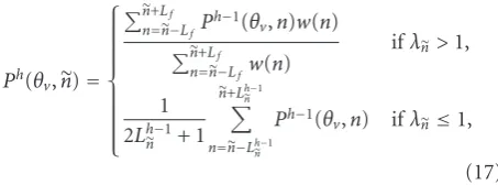
whereLfis the fixed window span factor and in our work it is set to 3 for isolated rings andLf =ceil(band ring width/2) + 1 for band rings, and J is a constant and was determined experimentally to be J = 660. For every faulty detector position in a particular view, the correction is made as
Ph(θ v,n)=
⎧ ⎪ ⎪ ⎪ ⎪ ⎪ ⎪ ⎪ ⎪ ⎨ ⎪ ⎪ ⎪ ⎪ ⎪ ⎪ ⎪ ⎪ ⎩
n+Lf
n=n−LfPh−1(θv,n)w(n) n+Lf
n=n−Lf w(n)
ifλn>1,
1 2Lh−1
n + 1
n+Lh−1
n
n=n−Lh−1 n
Ph−1(θ
v,n) ifλn≤1,
(17)
where the iteration number is indicated by h, and λh−1 n andLhn−1 are weighting factor and span factor, respectively, obtained from Ph−1(θ
v,n) at the detector position j = n. Here, for the first iterationP0(θ
v,j)=P(θv,n) andL0ncan be chosen any integer value from 3 to 9. The corrected sinogram after the end of iterations,h, is denoted asP(θ,n). Multistage implementation of the ring suppression (detection and correction) algorithm is possible by treating this corrected sinogram (P(θ,n)) as corrupted sinogram (P(θ,n)) and repeating the whole process again. The advantage of the multistage algorithm is to identify and remove any correction algorithm generated secondary edges in the sinogram.
3. Experimental Results
The schematic of a μ-CT system for acquisition of the projection or sinogram data of a desired object is shown in
Figure 4. The test images were acquired with a home made
micro-CT which consists of a flat-panel detector (C7943CA-02, Hamamatsu, Japan) and a microfocus X-ray tube (L8121-01, Hamamatsu, Japan). The microfocus X-ray source is a sealed tube with a fixed tungsten anode having an angle of 25◦ against the electron beam and with a 200μm-thick beryllium exit window. The emitted X-ray beam span angle is about 43◦. The source has a variable focal spot size from 5μm to 50μm depending on the applied tube power (Watt or kVp×mA). The maximum tube voltage and tube current are 150 kVp and 0.5 mA, respectively. The microfocus X-ray source has been operated in a continuous mode with an Al filter with a thickness of 1 mm. The flat-panel detector consists of a 1216 ×1216 effective matrix of transistors and photodiodes with a pixel pitch of 100μm and a CsI:Tl scintillator. The CsI:Tl has a columnar structure with a
Limited FOV data
Rotation Rotation
Full FOV data
Object
holder Motor Objectholder
controller Micro-focus X-ray source X-ray tube controller Flat-panel detector Processing computer z y x
Figure4: A schematic of aμ-CT system for acquisition of sinogram
data.
typical diameter of about 10μm and a thickness of 200μm. A computer-controlled rotating system was adopted in the object holder to achieve a cone-beam mode scan in the micro-CT. The precision of the rotational motion is 0.083◦ which allows the number of views to be larger than 4000. The data are contribution from Department of Biomedical Engineering of Kyung Hee University, Korea.
The performance of our algorithm is first tested using synthetic images and ring patterns. This facilitates the use of an objective index-, for example, peak signal-to-noise ratio (PSNR), based evaluation of an algorithm. To demonstrate quantitative performance, computer-generated various random ring patterns of different strengths (Ring-1– Ring-6) were added to the test imagesImage-1 and Image -2 sinograms so as to obtain the corrupted sinograms. The index PSNR is defined as
PSNR=10 log
I2 MSE
dB, (18)
where I is the peak intensity of the clean image and it is 1 for an image normalized in the range [0,1]. The mean-squared error (MSE) between the imagesI(m,n) andIc(m,n) is calculated as
MSE= 1
N1×N2 N1
m=1 N2
n=1
[I(m,n)−Ic(m,n)]2, (19)
whereN1andN2are the number of rows and columns in the input images, respectively. For the wavelet-Fourier method wname = db42,L = 4, andσ =3 were chosen to correct these synthetic images. The performances of the proposed and wavelet-Fourier [16] methods are shown inTable 1. As can be seen, the PSNRs of the wavelet-Fourier method are significantly lower than those of the proposed method. This implies that our method can remove rings more efficiently with lesser distortion imparted to the corrected images.
Det
ect
or
position
450
50 150 250 350
884 885 886 887 888 889 890 891 Views Miscalibrated detector Strong defective detector defective detector Light (a) Det ect or position 450
50 150 250 350
Views 311 312 313 314 315 316 317 318 Miscalibrated detector (b) 450
50 150 250 350
Views
Miscalibrated and defective band of
detectors 298 300 302 304 306 308 310 312 314 Det ect o r positio n (c) 450
50 150 250 350
Views 0. 4 0. 6 0. 8 1 1. 2 1. 4 1. 6 1. 8 2 Good detector Miscalibrated detector Strong defective detector defective detector Light Int ensit y (d) 450
50 150 250 350
Views 0.94 0.95 0.96 0.97 0.98 0.99 1 1.01 1.02 1.03 1.04 Good detector Miscalibrated detector Int ensit y (e) 450
50 150 250 350
Views 2. 8 3 3. 2 3. 4 3. 6 3. 8 4 4. 2 Good detector Miscalibrated and light defective band of detectors Int ensit y (f)
Figure5: Various types of sinogram data investigated by the proposed algorithm. Cropped view of the sinogram showing (a) strong and
light defective detector elements along with a miscalibrated one, (b) isolated miscalibrated detector element, (c) band of detector elements where both defective and miscalibrated detectors are present; (d), (e), and (f): plot of corresponding detector element responses.
performance of the algorithm is also tested when the stated types of detector elements are present in a contiguous fashion. The maximum width of the band ring considered is 15 pixels (in case of cow bone,Figure 7(h)).
Since the corrected image quality much depends on the accuracy of the detection process, there should be some evaluation parameters by which we can measure the strength of a detection algorithm. We choose the parameters like sensitivity (Sn), specificity (Sp), and accuracy (Ac) for this purpose. The definitions of these parameters are given by
Sn=Detected true negative
Actual true negative ×100%,
Sp=Detected true positive
Actual true positive ×100%,
Ac=Detected true negative + Detected true positive Actual true negative + Actual true positive
×100%,
(20)
where the actual true negative means the number of actual faulty detectors and the detected true negative is the number of detected faulty detectors. In the same way, the actual true positive and the detected true positive refer to the actual number of good detectors and the detected number of good detectors, respectively. The actual true positives are determined by visual inspection of the projection data.
(a) (b)
(c) (d)
(e) (f)
(g) (h)
Figure6: Reconstructed original images corrupted by ring artifact ((a): Water phantom, (c): Contrast phantom, (e): Electrolytic capacitor-1,
(a) (b)
(c) (d)
(e) (f)
(g) (h)
Figure7: Reconstructed original images corrupted by ring artifact ((a): Rat chest, (c): Rat abdomen-2, (e): Trabecular bone, (g): Cow bone)
(a)
“db42”,L=4,σ=10
(b)
Span factor=5
(c)
Span factor=7
(d) (e)
Figure8: Reconstructed images of Rabbit Bone with an Implant from the corrected sinogram using different methods. (a): Original image,
(b): Wavelet-Fourier method, (c): MA method, (d): Median method, and (e): Proposed method.
a distortionless image it requires 100% specificity. The accuracy will be 100% if both the sensitivity and specificity are 100%. Table 2 shows these parameters computed for various images. It is clear fromTable 2 that except for two images our proposed algorithm achieves 100% sensitivity, where the specificities and accuracies for most of the images are close to 100%. Overall, the proposed method can be regarded as a highly accurate scheme for the identification of ring generating detector elements.
Next, we present results of the proposed correction algorithm and compare its performance with other reported techniques. Since for real images (having no reference image) it is hard to find a suitable objective index, we prefer the visual inspection method for quality evaluation. The original phantom and capacitor images with ring artifact and their corresponding corrected images using the proposed method are shown in Figure 6. And the original small animal (live rat) and cow bone images corrupted by ring artifact and their corresponding corrected images by the proposed method are presented in Figure 7. It is to be noted that the original images are corrupted by both single and band rings. As can be seen from Figures 6 and 7, all the reconstructed images after sinogram correction are clearly ring-free and there is no visible additional distortion imparted by the proposed algorithm. Figures8and9show the original ring corrupted (Figures8(a)and9(a)) and the
(a)
“db41”,L=2,σ=7
(b)
Span factor=4
(c)
Span factor=7
(d) (e)
Figure9: Reconstructed images of Rat Abdomen-3 from the corrected sinogram using different methods. (a): Original image, (b):
Wavelet-Fourier method, (c): MA method, (d): Median method, and (e): Proposed method.
selection of these parameters. On the contrary, in case of our algorithm the threshold is adaptive with the variation of the information content in a frame. In the MA method [11], the span factor may be varied (in Figures8(c)and9(c), the span factors are 4, 5, resp.) to produce the best possible result. In MedF method, the window length is fixed (e.g., 15 was used for both in case of the results presented here), whereas in the VWMA and WMA methods the window size and weighting factor are self-adaptive according to the degree of error introduced. Moreover, in strict sense, there is no detection algorithm in the MA and MedF methods and the correction is done using the normalization approach [12] with the normalizing factor obtained from the original and corrected mean curves. Therefore, the MA and MedF methods cannot eliminate rings with varying intensity as evident from Figures8 and9. The beautiful results of the proposed technique is due to the accurate detection process and the smart correction procedure that ensures different level of correction at different views even at a single detector.
4. Conclusion
This paper has dealt with a novel ring artifact suppression method from the images of digital X-ray detector-based CT system. As the ring artifacts in the reconstructed CT image are manifested as vertical stripe artifacts in the sinogram,
Table1: Performance comparison of the two methods in terms of
PSNR.
Test image and ring PSNR in dB
Input PSNR
Wavelet-Fourier method
Proposed method
Image-1andRing-1 09.5703 16.1429 36.6614
Image-1andRing-2 12.4786 19.1367 34.4324
Image-1andRing-3 14.0023 12.5946 36.5501
Image-2andRing-4 15.8423 15.3245 36.5782
Image-2andRing-5 14.3748 19.3332 37.7361
Image-2andRing-6 11.8517 22.2354 35.7955
Table2: Accuracy of the proposed detection algorithm.
Test Image Performance Parameters for Ring Detection Sensitivity
(%)
Specificity
(%) Accuracy (%)
Capacitor-1 100.00 99.57 99.59
Contrast Phantom 100.00 99.92 99.92
Trabecular Bone 100.00 100.00 100.00
Cow Bone 97.17 98.65 99.60
Water Phantom 100.00 99.75 99.75
Rabbit Bone with
Implant 100.00 98.82 98.85
Resolution Phantom 100.00 99.75 99.92
Rat Chest 100.00 100.00 100.00
Rat Abdomen-1 100.00 100.00 100.00
Rat Abdomen-2 100.00 100.00 100.00
Rat Abdomen-3 100.00 99.92 99.92
Capacitor-2 91.67 99.59 99.84
All synthetic images 100.00 99.52 99.53
conventional moving average (MA) filter-based approaches, the window size for the VWMA or the weight for the WMA is determined dynamically in proportion to the degree of error in the response of a detector element. Therefore, the blurring effect is not observed using these filters. As the intensity of the artifact may vary in a detector, the correction filter has been operated on every faulty detector position to correct every pixel adaptively, unlike the conventional mean curve-based normalization technique. The elegance of the proposed method is that it does not handle any detector position that is not detected in the detection process. Therefore, no distortion is introduced by the operator in the good detector positions. The performance of the proposed algorithm has been tested and compared with other reported algorithms using both the synthetic and real CT images. The synthetic image were used to measure the detection accuracy of the proposed algorithm and to observe comparative performance using an objective index. The experimental results on ring generating stripe detection accuracy and ring removal efficacy on various types of synthetic and real CT images with different ring patterns have demonstrated that the performance of the proposed method is highly satisfactory. The comparative results have also revealed that the quality of the corrected reconstructed images by our method is significantly better than the comparing methods in this paper. The proposed ring suppression technique is particularly strong for the correction of fully and partially defective detector responses and is relatively weak for the cor-rection of miscalibrated detector responses. Classifying ring artifacts and developing class adaptive correction schemes are the topics for future research.
Acknowledgment
This work was supported in part by the National Research Foundation (NRF) of Korea funded by the Korean govern-ment (MEST) (no: 2009-0078310).
References
[1] A. C. Kak and M. Slaney, Principles of Computerized Tomo-graphic Imaging, SIAM, 2001.
[2] G. T. Herman, Fundamentals of Computerized Tomography, Springer, Berlin, Germany, 2nd edition, 2010.
[3] V. David, N. Laroche, B. Boudignon et al., “Noninvasive in vivo monitoring of bone architecture alterations in hindlimb-unloaded female rats using novel three-dimensional micro-computed tomography,”Journal of Bone and Mineral Research, vol. 18, no. 9, pp. 1622–1631, 2003.
[4] M. J. Paulus, S. S. Gleason, S. J. Kennel, P. R. Hunsicker, and D. K. Johnson, “High resolution X-ray computed tomography: an emerging tool for small animal cancer research,”Neoplasia, vol. 2, no. 1-2, pp. 62–70, 2000.
[5] S. C. Lee, H. K. Kim, I. K. Chun, M. H. Cho, S. Y. Lee, and M. H. Cho, “A flat-panel detector based micro-CT system: performance evaluation for small-animal imaging,”Physics in Medicine and Biology, vol. 48, no. 24, pp. 4173–4185, 2003. [6] J. Sijbers and A. Postnov, “Reduction of ring artefacts in high
resolution micro-CT reconstructions,”Physics in Medicine and Biology, vol. 49, no. 14, pp. N247–N253, 2004.
[7] D. Prell, Y. Kyriakou, and W. A. Kalender, “Comparison of ring artifact correction methods for flat-detector CT,”Physics in Medicine and Biology, vol. 54, no. 12, pp. 3881–3895, 2009. [8] Y. Kyriakou, D. Prell, and W. A. Kalender, “Ring artifact
correction for high-resolution micro CT,”Physics in Medicine and Biology, vol. 54, no. 17, pp. N385–N391, 2009.
[9] X. Tang, R. Ning, R. Yu, and D. Conover, “2D wavelet-analysis-based calibration technique for flat panel imaging detectors: application in cone beam volume CT,” in Medical Imaging 1999: Physics of Medical Imaging, Proceedings of SPIE, pp. 806–816, San Diego, Calif, USA, February 1999.
[10] J. A. Seibert, J. M. Boone, and K. K. Lindfors, “Flat-field correction technique for digital detectors,” inMedical Imaging 1998: Physics of Medical Imaging, Proceedings of SPIE, pp. 348–354, San Diego, Calif, USA, February 1998.
[11] M. Boin and A. Haibel, “Compensation of ring artefacts in synchrotron tomographic images,”Optics Express, vol. 14, no. 25, pp. 12071–12075, 2006.
[12] R. A. Ketcham, “New algorithms for ring artifact removal,” in Developments in X-Ray Tomography V, Proceedings of SPIE, San Diego, Calif, USA, August 2006.
[13] X. Tang, R. Ning, R. Yu, and D. Conover, “Cone beam volume CT image artifacts caused by defective cells in x-ray flat panel imagers and the artifact removal using a wavelet-analysis-based algorithm,”Medical Physics, vol. 28, no. 5, pp. 812–825, 2001.
[14] F. Sadi, S. Y. Lee, and M. K. Hasan, “Removal of ring artifacts in computed tomographic imaging using iterative center weighted median filter,”Computers in Biology and Medicine, vol. 40, no. 1, pp. 109–118, 2010.
[15] C. Raven, “Numerical removal of ring artifacts in microto-mography,”Review of Scientific Instruments, vol. 69, no. 8, pp. 2978–2980, 1998.