R E S E A R C H
Open Access
Multi-view alignment with database of
features for an improved usage of high-end 3D
scanners
Francesco Bonarrigo
1,2, Alberto Signoroni
1,2*and Riccardo Leonardi
1,2Abstract
The usability of high-precision and high-resolution 3D scanners is of crucial importance due to the increasing demand of 3D data in both professional and general-purpose applications. Simplified, intuitive and rapid object modeling requires effective and automated alignment pipelines capable to trace back each independently acquired range image of the scanned object into a common reference system. To this end, we propose a reliable and fast
feature-based multiple-view alignment pipeline that allows interactive registration of multiple views according to an unchained acquisition procedure. A robust alignment of each new view is estimated with respect to the previously aligned data through fast extraction, representation and matching of feature points detected in overlapping areas from different views. The proposed pipeline guarantees a highly reliable alignment of dense range image datasets on a variety of objects in few seconds per million of points.
Keywords: 3D modeling pipelines, Geometric feature extraction, Feature description and similarity, Partial shape matching, Range image datasets, 3D scanner usability
Introduction
In the last years, 3D datasets acquired with modern opti-cal scanning devices (either based on structured light projection or laser beams) increased their spatial res-olution. Other primary features, such as accuracy and acquisition speed, have also been improved. Scanner are decreasing their size and weight and their usage is expected to become more and more intuitive and uncon-strained, such as the use of digital cameras. This would be desirable in response to an increasing demand of “3D” for today professional applications (industry and design, medicine, cultural heritage, robotics, mechanics, build-ing constructions. . .) as well as for soon to come web applications.
The first step toward the 3D modeling of a physical object is the acquisition of multiple scans from different viewpoints of the surface of interest. After the acquisition, each set of 3D data (either composed by range images or point clouds) needs to be accurately aligned (or registered)
*Correspondence: [email protected]
1Information Engineering Dept., University of Brescia, Brescia, Italy 2CNIT - UoR at University of Brescia, Brescia, Italy
into a common coordinate system [1-3]. Aligned datasets are then fed to a subsequent step of the object modeling pipeline [4], with the initial alignment quality influencing the accuracy and fidelity of the resulting object model.
Under the basic hypothesis of a certain degree of over-lap among different views, the registration problem can be conceptually split into a cascade of coarse and fine alignments. Even if they can be considered as instances of a more general class of problems called ‘shape corre-spondence’ [5], they are different in nature and require distinct solving approaches. The goal of coarse alignment is to roto-translate each independently positioned scan (an example is shown in Figure 1) so that the entire dataset can be roughly brought into a common reference system (as shown in Figure 2). This takes place without making any assumption on the initial viewpoints. A second stage fine alignment is then used to accurately register the scans from the first approximate alignment.
Both coarse and fine approaches can be performed pair-wiseor multi-view). Solutions within the first class only exploit the information present in the overlapping area with respect to a single range image to determine sep-arately the alignment between each pair of views, while
Figure 1A set of scrambled views composing the Dolphin object prior coarse alignment application.
multi-view alignment integrates all the available overlap-ping information collected from all acquired scans and exploits it in order to estimate the correct alignment. Even though pairwise and multi-view coarse alignment approaches may seem equally effective to accomplish their role, this is not true anymore in a practical acquisi-tion settings. In fact, pairwise coarse alignment requires each couple of subsequent views in a dataset to possess a certain amount of overlap (from now on we address such requirement as the overlap constraint). This can be obtained by either forcing the operator to devise in advance an acquisition path which complies with the overlap constrain (thus limiting the scanner usability),
or by manually reordering the original acquisition path as a preprocessing step (which may represent a tedious and time consuming process). On the contrary, multi-view approaches allow a more unconstrained usage of the acquisition devices, in that the overlap condition can be relaxed so that each incoming scan is only required to possess a certain overlap with respect toanyof the pre-viously aligned range data. This effectively extends the applicability of automated coarse alignment to a greater number of less constrained acquisition paths. From now on, we shall address as unchained path any acquisi-tion path which abides by the previously stated relaxed requirement.
In this work, our main focus is on the description of a new multi-view coarse alignment method suited for high-resolution datasets, specifically designed to fulfill the following requirements: (1) it should improve the scanner usability by allowing the operator the freedom to choose the acquisition path, (2) it should prove to be equally effec-tive regardless to the nature of the acquired object as well as its size, (3) the alignments should be fast so as to give the user on-the-fly visual feedbacks during object digital-ization. We will see that effective multi-view alignment solutions can be designed starting from an efficient pair-wise alignment technique. In this paper we present the proposed solutions in two main parts: pairwise alignment (Section “Pairwise alignment technique ’’) and multi-view alignment (Section “Multi-view alignment pipeline”). In particular we propose:
– for Pairwise alignment:
(1) a multiscale feature extraction technique capable of identifying feature points and their scale (Section “Feature extraction”);
(2) a lightweight feature signature devised to quickly reduce the matches space (Section “Feature description”);
(3) a matching chain developed to progressively skim the correspondence space (Sections “Feature matching” and “Correspondence test and selection”);
– for Multi-view alignment:
(1) the definition of a feature database for the multi-view alignment (Section “Feature database update”);
(2) the use of a global adjustment solution to optimize the alignment obtained through the proposed multi-view pipeline (Section “Global adjustment”);
Each block of the pipeline has been tested in isola-tion (Secisola-tion “Comparative tests”). An evaluaisola-tion of the entire pipeline performance is proposed (Section “Experimental results”) on a set of range image datasets, presented in Section “Acquired datasets”, represent-ing different objects taken durrepresent-ing real acquisition campaigns. In particular, in-depth comparative tests with respect to alternative solutions have been made both on the feature extraction and description phases (Section “Feature extractor and descriptor comparison ’’) and on the correspondence test and selection solutions (Section“Correspondence test technique comparison ’’). Overall performance evaluations are presented in (Section “Experimental results”) and organized accord-ingly to the structure of the proposed solutions: Section “Pairwise alignment results ’’ presents a
quantita-tive evaluation of the pairwise alignment performance in terms of success rate and computational complexity, while Section “Multi-view alignment pipeline” presents a quan-titative evaluation of the multiview alignment in terms of success rate, computational complexity and alignment error. Conclusion are drawn in Section “Conclusions”. The present paper builds on our conference paper [6], extend-ing it in several parts. The experimental section has been widened considerably, while performance evaluation of each pipeline block in isolation has been performed.
Related work
kind and dimension. Related works are those presented by Li and Guskov [19] and Lee et al. [20] which introduced extensions of Lowe’s 2D SIFT [21] to 3D datasets. Their approach has been subsequently exploited by Castellani et al. [22] and Bonarrigo et al. [6]. SIFT-related feature description distinctiveness against Spin Images has been compared in [23]. Thomas and Sugimoto [24] proposed to use the reflectance properties for images registra-tion to better perform on featureless images. In feature-based approaches, feature points are usually associated to descriptors, which ideally should associate an unambigu-ous signature to each feature, which is fast to compute and robust to any viewpoint rotation as well as to variations of point density on the image. Li and Guskov [19] pro-posed a descriptor based on a combination of local Dis-crete Fourier transform and DisDis-crete Cosine transform to describe the neighborhood of each feature point. Gelfand et al. in [3] proposed the use of volumetric descriptors, that is the estimation of the volume portion inscribed by a sphere centered at a point of the surface. Castellani et al. [22] proposed a statistical descriptor based on a hidden Markov chain that is trained through its neighbor-hood. Despite scan alignment and similar problems have been thoroughly explored in the literature, meaningful comparisons remain somehow difficult to accomplish for several reasons: the heterogeneity of each approach, the different way in which they are combined into functional alignment pipelines, the variability of the addressed per-formance and application requirements, the differences of test datasets both in terms of representation primi-tives (range images, point clouds, meshes, etc.) and data characteristics (resolution, noise, etc.) related to the dif-ferences in data acquisition setup and scanning hardware. In particular, even if each block of a feature-based align-ment pipeline (feature extraction, description, matching, correspondence selection and transform estimation) can be tested in isolation with respect to alternative solutions (we will do this in Section “Comparative tests”), criti-cal interdependencies exist among the different pipeline blocks. In this work we adopted design criteria which take full account of such interdependency, according to what has been recognized in reference reviewing work [15,17]. Bustos et al. [17] indicated that a complete and fair comparison of feature extraction and description techniques is unfeasible and that the specific application requirements should inspire and provide guidance for the design of application-driven solutions. Bornstein et al. [15] concluded their review by suggesting to avoid the design of pipelines composed by unnatural block com-binations. Another relevant aspect is that multiple-view coarse alignment solutions are usually proposed in liter-ature as simple extensions of pairwise approaches. This leads to a serious limitation on the usability of the acquisi-tion devices. The increased complexity of a multiple-view
coarse alignment has been recognized in [1] with a solu-tion proposed by model graphs and visibility consistency tests. An approach based on view trees has been adopted in [9] where multiple-view coarse alignment is obtained by maximization of inlier point pairs. However, these solu-tions do not allow interactive acquisition because they work on a graph of the pairwise matches once all the align-ments are completed, and this conflicts with the need of on-the-fly visual feedbacks. By exploiting the possibility of some range scanners to acquire views at high frame rate (e.g. Kinect and alike sensors), hand-held on-the-fly acqui-sition and alignment solutions have been proposed [25,26] with specific solutions for handling loop closure problems [27] or computational burden [28]. However, these inter-esting applications are still too far from today professional requirements of high point density and metric precision.
Pairwise alignment technique
Overview and notation
In this section we shall introduce some notation, as well as briefly summarize the alignment process. A range image can be conceived as the projection of a 2D image grid on a 3D target object surface and the acquisition of depth-related information from that surface. The result-ing dataset is a “structured” point cloud, that is a set of points lying in a 3D space, and associated to a pixel of the acquisition grid. We define a range image as a map I ⊂ Z2 → R ⊂ R3, where the domain Iis a rectangu-lar grid (usually corresponding to the CCD matrix), while the co-domainRcorresponds to the set of 3D points rep-resenting the acquired surface. Due to the limitations of the acquisition procedure (limited measure range, occlu-sions due to the object shape, etc.), not all pixel positions i∈Imay have a valid corresponding pointpi ∈R, there-fore only a subsetIV ⊆ Iof valid points is acquired for each image. We take advantage of range images data struc-ture in order to speed up the processing: in particular, by exploiting the image domainI, neighborhood informa-tion can be retrieved quickly and efficiently, while data processing is performed over the 3D target spaceR. An example of efficient processing obtained by exploitation of the 2D grid is the normal field estimation method we employ. For a given point c we exploit the 2D grid to identify its 8 closest neighbourspk, withk∈[ 0, 7], to esti-mate the normalnˆc. At first, for every valid pointpk the vectorsvk = pk−care computed. Then the outer prod-ucts between each valid couple of vectors(vk,v(k+2)%8)are determined. Once normalized, they are summed together and their average is set as the normal for pointc.
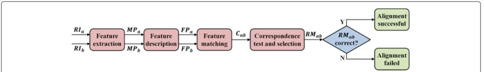
Figure 3The pairwise alignment system, composed by: feature extraction (Section “Feature extraction”), feature description (Section “Feature description”), feature matching (Section “Feature matching”), correspondence test and selection (Section “Correspondence test and selection”).
pair of range images RIa and RIb, the first step in the pipeline applies a multi-scale feature extraction method thoroughly described in Section “Feature extraction”, such that meaningful points MPa and MPb are identified on the respective surfaces. Following, each point in the sets MPaand MPbis associated with a signature, described in Section “Feature description ’’, which encodes neighbor-hood information with respect to the meaningful point. The signature is designed to be suitably discriminative and fast to compute. This way, two sets of feature points FPa and FPb are obtained. Correspondences between these 2 sets are then established through the matching pro-cess described in Section “ssec:featureMatching ’’, which exploits the signatures in order to identify pairs of com-patible feature points so that a correspondence set Cab is determined. Each correspondence c is constituted of a pair of feature points, one taken from FPa and the other from FPb. In the next phase, correspondences are grouped to form triplets, as described in Section “Cor-respondence test and selection”, and the ones which are most likely to be correct are collected in a triplet set Tab. We resort to triplets of correspondences since they contain the minimum number of points (that is, 6 3D coordinates, 3 of which lie in the reference system associ-ated to RIawhile the others lie in the one associated with RIb) for which a roto-translation matrix can be estimated, for instance applying the method described by Horn in [29]. The triplet setTabis then evaluated so that a sin-gle roto-translation matrixRMabis identified and verified with respect to its correctness.
Feature extraction
The feature extraction technique we adopt here is a mod-ified version of the approach proposed by Castellani et al. [22]. His approach is similar to the one introduced by Lee et al. [20], which can be in turn considered as a 3D exten-sion of the 2D multi-scale analysis proposed by Lowe [21]. Hereafter we shall summarize Lee’s approach, then we will highlight the modifications introduced by Castellani, as well as our own.
The approach from Lee et al. requires that: (a) given a range image RI, M filtered images G(r), at scales r ∈[ 1,M], are derived by applying Gaussian kernels of
growing dimension; (b) a set ofM−1 saliency mapsS(r) is derived from pairs ofG(r)at consecutive scales, from which a set of MP is identified. These MP are candidate features, and are associated with the scale at which they have been detected. To produce the filtered imagesG(r)at various scalesr∈[ 1,M], a geometric Gaussian filtering is applied to each valid pointpiin the RI, obtaininggi(r):
gi(r)=
pj∈B2σr(pi)
pj·e− pi−pj2
2·σ2
r
pj∈B2σr(pi)
e− pi−pj2
2·σ2
r
(1)
where B2σr
pi identifies the points within a euclidean distance 2σrfrompi. A filtered imageG(r)is thus defined as the set of pointsgi(r), withi ∈[ 1,|IV|]. As the kernel radiusσrincreases, details which size is smaller thanσrare smoothed out fromG(r)and, when the kernel size dou-bles, computations are performed on images subsampled by a factor two.
Once the filtered versions G(r) have been calculated, M− 1 saliency maps are derived. A saliency map is a 2D array of scalar values, obtained by pairwise subtrac-tion ofG(r)at adjacent scales. This retains only the details comprised between the two bounding scalesrandr+1, in other words it highlights features which dimension is comprised between the kernel sizesσrandσr+1. Saliency mapsS(r)= {si(r)}are calculated as follows:
si(r)=gi(r)−gi(r+1) (2)
The maximum values of each saliency mapS(r)are con-sidered to be MP and located through an iterative search where, once the greatest valid saliency value for S(r) is found, no other maximum can be selected within an inval-idation neighborhood region B2σr+1
pi. This prevents the selection of feature points which descriptors would partially overlap, since the descriptor size for features detected at scaleS(r)isσr+1.
pairwise difference and the normal associated to the orig-inal 3D point:
si(r)=nˆi,gi(r)−gi(r+1) (3)
This correction should help in reducing the saliency val-ues associated to points that, after the filtering, have moved away from their normal direction. We have found out, however, that such saliency correction (originally pro-posed for mesh data) needs to be corrected in order to apply it to range images and point clouds. Since these types of data usually contain a greater number of 3D points than mesh vertices, their normal field is more sub-ject to vary due to the filtering process. Therefore, in order to obtain a reliable saliency estimation, we propose to use the normal field associated to the filtered data itself:
si(r)=nˆi(r),gi(r)−gi(r+1) (4)
Although such a modification requires an estimation of the normal field for every filtered image G(r), we will demonstrate in Section “Feature extractors comparison” that it brings a significant performance boost with respect to feature localization.
This saliency estimation described in (4), brought a slight increment in performance with respect to the approach initially proposed in [6]. Once the set of MP has been computed, a number of tests on each meaning-ful point is performed in order to make sure that: (1) its neighbour points are well distributed and (2) it is not close to a border or hole, otherwise the associated descriptor would be incomplete; (3) it does not lie over a saliency ridge, because in such cases small variations in saliency
estimation may cause great variations of maximum local-ization. If any of these conditions is not met, the point is discarded from the set MP. Hereafter, for a neater and more compact notation we will omit unnecessary indices when things have general validity.
Feature description
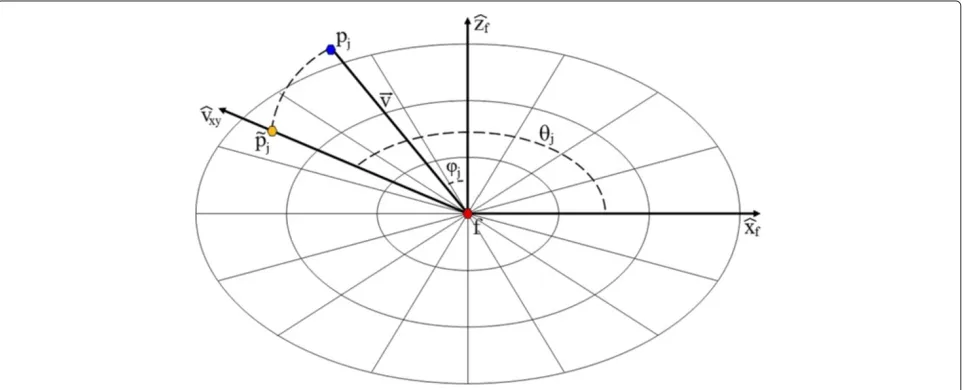
In order to search for correspondences between feature points belonging to different range images we rely on fea-ture descriptors. We propose to associate to each feafea-ture point f ∈ MP detected at scaleσr a descriptor which encodes information extrapolated from both the normal vectors and saliency data of the neighbour points pj ∈ Bσr+1(f). In summary, given a feature pointf, we define a polar grid spanning the tangent plane to f. This grid is composed of Mradial sectors and Langular sectors, as shown in Figure 4. Every neighbour point pj within Bσr+1(f)is associated to a grid sector, and for each sec-tor we compute two score values derived by the normal and saliency information. As a result, our descriptor is composed by 2×M×Lreal (floating point) values. Fol-lowing, we describe in more detail how the descriptor is computed.
At first, a local reference system xˆf,yˆf,ˆzf is centered
on f. Versor ˆzf is set toward the direction of the
fea-ture normalnˆf, while the span of{ˆxf,yˆf}identifiesPf, i.e.
the plane tangent to f. The direction ofxˆf is randomly
selected, whileˆyf = ˆzf × ˆxf. A polar grid of radiusσr+1 is then defined and subdivided intoMradial andL angu-lar sectors. We have empirically found that M = 3 and L=36 generate a distinctive signature, while allowing fast computation. Each pointpjbelonging toBσr+1(f)is then associated to a given sector of the polar grid by mapping pjon the planePf. This is represented in Figure 4 by the
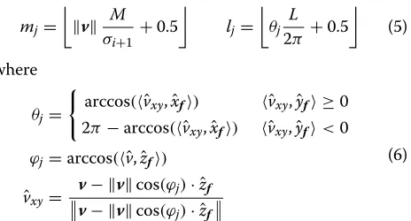
pointp˜j = f + v · ˆvxy, wherev = pj−f. The sector indexes(mj,lj)associated topjare computed as follows:
mj=
v M σi+1 +
0.5 lj=
θj
L
2π +0.5 (5)
where
θj=
arccos(ˆvxy,xˆf) ˆvxy,yˆf ≥0
2π−arccos(ˆvxy,xˆf) ˆvxy,yˆf<0
ϕj=arccos(ˆv,zˆf)
ˆ vxy =
v− vcos(ϕj)· ˆzf
v− vcos(ϕj)· ˆzf
(6)
Once each pointpj ∈ Bσr+1(f)has been associated to a sector, it is possible to computewf, the descriptor
asso-ciated to feature point f. At first, for each sector (m,l) the average normal vectornˆ(m,l)and saliencys(m,l)are computed (if a sector does not contain any point, it is con-sidered invalid). Then, given nˆf andsf respectively the
normal vector and the saliency value associated to the fea-ture pointf, the sector descriptorwf(m,l)is computed as
follows:
wf(m,l)=[n(m,l),s(m,l)]
n(m,l)=1.0−nˆ(m,l),nˆf
s(m,l)=1.0−s(m,l) sf
(7)
Each sector descriptorwf(m,l) will therefore contain
two scores (nands, both∈[ 0, 1]) related to how much the average normal and saliency values in each grid sector differ from the corresponding feature point values. The feature descriptor wf is therefore the set of theM× L
sector descriptorswf(m,l)thus calculated. Once each
fea-ture point has been associated to its descriptor, they are organized in the set FP for the subsequent processing stages.
The proposed descriptor is fast to compute since both normals and saliency information are already available (the latter being a byproduct of the extraction procedure described in Section “Feature extraction”) once the feature points have been identified. Moreover, it is moderately lightweight as it only requires 2×M×Lfloating point values. Nevertheless, it is enough selective as to allow to skim the correspondence space to a more treatable dimen-sion while retaining enough correct correspondences. In Section “Feature descriptor comparison” we will complete these observations by comparing our descriptor to the Spin Images introduced by Johnson [30] and by demon-strating its superior performance.
Feature matching
Given two feature sets FPaand FPb, estimated on differ-ent range images, the objective of this pipeline block is to
calculate all possible feature correspondences by match-ing the descriptors of each pair of features (fs ∈ FPa, fd ∈FPb), and subsequently select a subset of correspon-dences Cab which is likely to contain the correct ones. Figure 5 gives the reader an intuition on how feature similarities can define relevant matches.
In Section “Feature description ’’ we stated that the direction of xˆf is chosen arbitrarily for each feature
descriptor. This can be modeled with an unknown dis-placement factorL¯, withL¯ ∈[ 1,L], between the signatures of the same feature point on two different range images. We therefore compensate this indetermination by per-forming an operation similar to the circular correlation, in that one of the descriptors remain fixed, while the other is shifted along the circular direction forLtimes. At each rotation step a score is computed, and the maximum score value is selected as follows:
cscoresd =max¯l∈[1,L]
cscoresd (¯l) (8)
with
cscoresd (¯l)= M m=1 L l=1
nscoresd (m,l,¯l)·sscoresd (m,l,¯l)
nscoresd (m,l,¯l)=1−ns(m,l)−nd(m,¯l)
sscoresd (m,l,¯l)=1−ss(m,l)−sd(m,¯l)
Once all possible matches between the two feature sets FPa and FPb have been computed, we need to skim the matches set from its original size|FPa| · |FPb|to a more treatable dimension. We therefore define a correspon-dence setCabof sizeQas the list of correspondencescq found between FPa and FPb which possess the highest correspondence score. We decided to retain the best Q correspondences (in this work we useQ = 150), rather than fix a hard threshold for the score, since the score dis-tribution is not constant with respect to different image pairs. Within the set of Q best matches we have also verified that, in general, the majority of correct correspon-dences share the top positions of the ranking together with a small number of false matches (generated by inci-dental signature similarities). This means that we cannot “blindly” exploit the first correspondences of the ranking to estimate the roto-translation matrix between the views. We therefore introduce a robust selection step (described in the following section) to determine the most reliable correspondences within the setCab.
Correspondence test and selection
Figure 5Feature signatures.Upper part: two range images on which some feature points are highlighted with different colors. Below, graphical visualization in a red-blue scale of the signatures, contoured with their corresponding colors. The first two features (yellow and red) as well as the last two ones (orange and pink) have well matching descriptors.
(a triplet) need to be identified within the setCab. Each triplettis defined as follows:
t=cg,ch,cj
, with ⎧ ⎪ ⎨ ⎪ ⎩
cg,ch,cj∈Cab g,h,j∈[ 1,Q] g=h=j
(9)
Solutions such as RANSAC [12] and similar ones are known to be effective solutions in performing these type of searches, however it is also known that the number of trials required to determine the correct model (in our case, a triplet) grows exponentially with respect to the proportion of outliers in the set. Unfortunately, in our scenario the number of inliers within the setCab is likely to be small. Indeed, it is below 15% in more than half of the considered cases, as we will show in Section “Correspondence test technique comparison ’’. There-fore we can expect the computational burden of RANSAC-style approaches to be high for such scenario.
Alternatively, we propose a robust selection procedure designed to progressively skim the correspondences so that the computational cost is kept low at each stage. The procedure consists of three steps: (1) every correspon-dence within Cab is validated against each other and a score is calculated for each pair of matches; (2) for each triplet of correspondences a score is computed based on the three pairwise scores previously calculated, and a sub-setTabofUbest triplets is retained; (3) for each triplet in Tab, a roto-translation matrixRMis estimated and applied to the feature set FPb, corresponding points are searched within image RIa. The triplet which collects the highest number of such corresponding points is considered as the more reliable estimate. The above three steps are now described in detail.
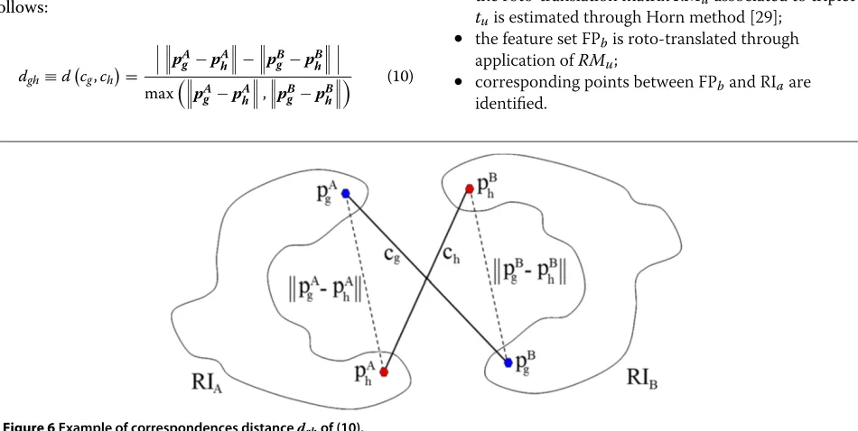
(1) In order to validate each correspondence with respect to the others we exploit the rigidity constraint, which states that the distance between two points subject to an Euclidean transformation remains constant. We also introduce the concept of relative distance between a pair of correspondences, illustrated in Figure 6, and defined as follows:
dgh≡d
cg,ch
=
pAg −pAh−pBg −pBh
maxpAg −pAh,pBg −pBh
(10)
Due to the normalization term at the denominator, the relative distance is bounded between 0 (same distance) and 1 (maximum distance). The evaluation of the rela-tive errors allows to perform a more unbiased ranking than that it would be with absolute errors (which tend to favor correspondence pairs of features which are close together). Once the relative distances have been esti-mated, they are organized into a Q × Q matrix DM:
DM=
⎡ ⎢ ⎢ ⎢ ⎢ ⎢ ⎢ ⎢ ⎣
0 d12 d13 · · · d1Q
d21 0 d23 d2Q
d31 d32 0 d3Q ..
. . .. ...
dQ1 dQ2 dQ3 · · · 0
⎤ ⎥ ⎥ ⎥ ⎥ ⎥ ⎥ ⎥ ⎦
(11)
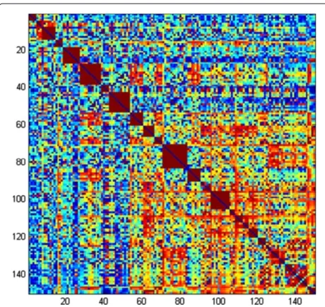
DMis symmetric (dhg=dgh), and possesses zeros over its main diagonal (dgg = 0,∀g ∈[ 1,Q]). An example of how such matrix looks like is presented in Figure 7.
(2) OnceDMis calculated, the triplet space is skimmed by determining the setTabofUtriplets (we setUto 25) which present the maximum value of the following score:
tscore=1− dgh+dhj+djg 3
g,h,j∈[ 1,Q] g=h=j (12)
Similarly to the skim procedure described in the previous section, this triplet skim procedure is able to retain the triplets made of correct matches in the highest positions of the ranking.
(3) In order to determine the most correct triplet within the set Tab, for eachtu ∈ Tab,u ∈[ 1,U] the following steps are performed:
• the roto-translation matrixRMuassociated to triplet tuis estimated through Horn method [29];
• the feature set FPbis roto-translated through application ofRMu;
• corresponding points between FPband RIaare identified.
Figure 7A distance matrixDM: blue dots represent low relative distance, while red ones identify distant matches.The red square clusters present along the diagonal are generated whenever evaluating pairs of correspondences that share one feature point (leading to a relative distance of 1).
The triplet¯twhich is found to possess the higher num-ber of corresponding points is considered as the one that is most likely to be correct. Its associated roto-translation matrixRM¯ is thus refined by taking into account all the corresponding points just estimated. At last, the obtained alignment is tested by selecting a subset of points from RIb, roto-translating them throughRM¯ , and verifying that at least a given percentage of points find a correspondence in RIa. If the number of matches is above this threshold, image RIkis considered as successfully aligned to the pre-vious one. Coherently with the view overlap constraint we set that threshold to 20%. As we will demonstrate in Section “Correspondence test technique comparison ’’, given the typical proportion of inliers for the setCab, the speed of our approach outperforms both RANSAC [12] as well as its descendant PROSAC [31] in determining the best triplet.
Multi-view alignment pipeline
As we will see in the experimental sections, the described pairwise alignment pipeline, even compared to other solutions, presents good performance and is suitable for automatic alignment of dense range scans in terms of computational speed and robustness (successful align-ment rate). Nevertheless, in order to reconstruct an entire object through such a pipeline, we would need to either define a chained acquisition path for which every con-secutive image pair complies with the overlap constraint
(thus limiting the scanner usability), or manually reorder the scans prior to applying the alignment (a tedious, time consuming and necessarily off-line operation). Therefore, from both a conceptual and practical point of view the chained path assumption turns out to be a limitation to the scanner usability.
For instance, imagine that an operator is using a scanner to acquire a human statue, trying to abide by the policy imposed by the overlap constraint. He starts acquiring the front of the statue (chest, belly, etc.), then progressively moves toward the back. At a certain point, however, he realizes that some region on the belly was not acquired properly, creating a “hole” in the digital model. He there-fore decides to acquire another range image on the front so that the hole can be properly filled. However, in order to comply with the overlap constraint he would need to capture more range data in regions he has already scanned to create a path between the back and the belly of the statue. It would be much simpler if he could fol-low anunchainedacquisition path, as defined in Section “Introduction”. Another advantage of an unchained path multi-view alignment with respect to the pairwise approach is the fact that overlapping regions from pre-viously aligned views can be cumulated to improve the chances of alignment: one view may not present enough overlap with respect to all the previously acquired ones, in such case any pairwise alignment attempt is likely to fail due to lack of reliable correspondences or because the 20% overlap requirement stated in Section “Correspondence test and selection ’’ is not met although the union of overlapping regions taken from different views may contain enough overlap (as well as reliable correspondences) to achieve the alignment.
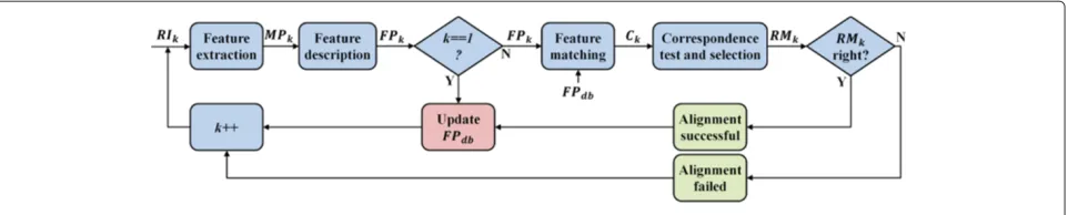
We then extend the pairwise approach by working with a database of features (indicated with FPdb) which collects the feature sets associated to all the previously aligned range images, so that the feature set associated to the cur-rent range image FPk is matched to the database FPdb. Figure 8 illustrates the block diagram of the multi-view alignment pipeline we propose. With respect to the stages described in Section “Pairwise alignment technique ’’, we need to introduce a new block (in red in Figure 8), which is responsible of updating the feature database.
Feature database update
Figure 8Block diagram representing the multi-view alignment system.
between the feature sets, in order to effectively curbing the database growth:
FPdb= k−1
i=1
FPi (13)
To do so, for each feature set FPk that needs to be inserted in inserted in the database FPdbwe identify any corresponding appears in the same 3D position (that is, closer than 1/3 of the feature signature radius). For each pair of concurrent features we select a single represen-tative based on the similarity of the feature normal with respect to the acquisition direction. In fact, we assume that such features possess better signatures, since their neighborhood is usually less afflicted by occlusion issues. We also associate to each representative apresence list, that is a list of all the range images in which that feature appears: this list is exploited during the triplet verifica-tion phase (described in Secverifica-tion “Correspondence test and selection”) to determine on which range images the test has to be performed.
Global adjustment
After having successfully applied the described multi-view coarse registration technique to a given dataset, we have the possibility to complete the alignment process toward a high-precision object modeling with a fine alignment and/or global adjustment step. Considering the multiple view nature of our problem, a multi-view fine alignment technique should be used to prevent residual errors to propagate along the alignment path (e.g. closure problems for objects with cylindrical symmetry). Among several methods present in literature we used an approach we recently proposed [32] which is suitable to accurately align sets of high-resolution range images, also directly starting from the coarse aligned dataset. This is particu-larly suitable in cases a chained pairwise fine alignment (e.g. using ICP) is prevented by the absence of a chained path. Our approach is based on the ‘Optimization-on-a-Manifold’ framework proposed by Krishnan et al. [33], to which we contribute with both systemic and computa-tional improvements. The original algorithm performs an error minimization over the manifold of rotations through
an iterative scheme based on Gauss–Newton optimiza-tion, provided that a set of exact correspondences is known beforehand. As a main contribution we relaxed this requirement, allowing to accept sets of inexact correspon-dences that are dynamically updated after each iteration. Other improvements were directed toward the reduc-tion of the computareduc-tional burden of the method while maintaining its robustness. The modifications we have introduced allow to significantly improve both the con-vergence rate and the accuracy of the original technique, while boosting its computational speed [32].
Acquired datasets
In order to compare each new building block of our pipeline in Section “Comparative tests”, as well as to evaluate both the pairwise and multi-view alignment per-formances in Section “Experimental results”, we consider a number of meaningful datasets that we acquired with a commercial high-resolution structured-light scanner (1280×1024 pixel CCD, i.e. potential 1.3M points/RI). The acquired datasets correspond to 14 scanned objects for a total of 300 range images, that is 286 RI pairs. They are shown in Figure 9, as they appear after suc-cessful alignment, with different colors associated to each range scan (naturally high color mixing due to scan inter-penetration is present). To make the pairwise and multi-view approaches fully comparable, among all the possible unchained acquisition paths a chained path has been determined and followed for each dataset. It is worth not-ing that for multi-view alignment a chained path can be considered as a regular element (with no special proper-ties or distinction) of the set of unchained paths (accord-ing to the definition given in Section “Introduction”). In addition, we will also consider alternative unchained paths to further evaluate the multi-view pipeline. The consid-ered objects are related to cultural heritage (statues and high-reliefs) and biomedical (orthodontic moulds) appli-cation fields, they have been chosen to represent well dif-ferentiated aspects and geometric properties, variegated feature dimensions, morphology and numerosity.
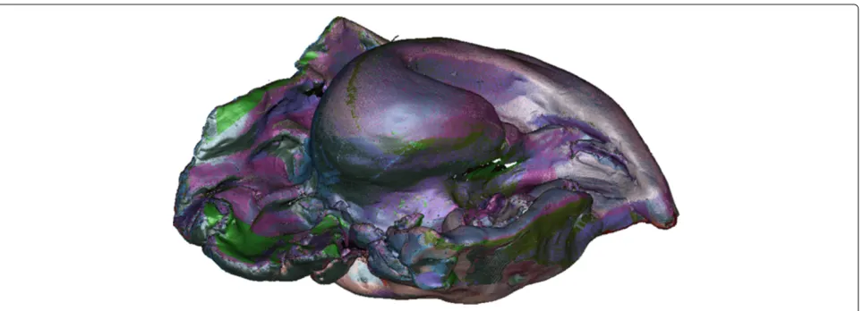
Figure 9The test datasets: Decoration, Angels, Mould 1, Mould 2, Dog, Cherub, Dolphin, Mould 3, Mould 4, Platelet, Capital, Rose, Hurricane, Venus.
surface of interest, the amount of overlap between the images can vary a lot due to the implicit characteris-tics of the surface that is being acquired: if the surface is quite planar, as for the Angels dataset, the maximum overlap is limited to 30%, whereas for datasets particu-larly affected by occlusion phenomena, such as the Rose dataset, many images cover the same area from different viewpoint angles, thus increasing the region overlap up to 80%. However, in these cases, an higher overlap does not necessarily imply an easier alignment, since the views can be heavily affected by holes which may cause instability in the feature localization as well as a degraded reliability of the computed descriptors for the features close to the hole borders.
Comparative tests
The pipeline we proposed in Section “Pairwise alignment technique” may appear to be constituted by independent blocks, thus easily interchangeable with alternative ones. However, as anticipated in Section “Related work”, a cer-tain degree of interdependency is present. In fact, our descriptor incorporates the saliency information, which is obtained during the multi-scale analysis performed during the extraction phase. A more subtle dependency regards the correspondence skim procedure: the number of correct correspondences that is obtained at the end of the matching block can be very limited, therefore the skim procedure has to be very reliable. This is the rea-son for which we came out with our own skim procedure rather than relying on heuristic approaches, which usu-ally have more stringent assumptions with regard to the number of inliers within the correspondence set. These considerations are to be taken into account when trying to compare the performance of each pipeline block: sub-stituting a given technique for another one, extrapolated from a different framework, may result in performance degradation. With these considerations in mind, we now propose a number of comparisons of our pipeline stages with respect to other works presented in the literature. We tried to identify solutions that may individually fit into
our pipeline in order to reduce performance degradation effects due to technique unsuitability.
In Section “Feature extractor and descriptor compari-son” we evaluate both the feature extractor (proposed in Section “Feature extraction”) and descriptor (introduced in Section “Feature description”) with respect to simi-lar approaches on a number of different scenarios we devised, while in Section “Correspondence test technique comparison” we evaluate our correspondence skim pro-cedure (described in Section “Correspondence test and selection”) with respect to other solutions by comparing both precision and computational efficiency. All the com-parisons presented in this section have been performed on the same platform described in Section “Pairwise align-ment results”.
Feature extractor and descriptor comparison
In order to assess the performance of the extraction and description blocks of our pipeline, we devised a number of test scenarios. Hereafter we state what is the objective we pursue for each block; then we describe the test scenarios. In order to compare our feature extraction technique with respect to the others, we aim to assess the capabil-ity to detect salient points in the same position, regardless to the possible variations that the surface may undergo due to various effects. We therefore devised three differ-ent scenarios in which we assess the feature repeatability with respect to: (1) noise added to the surface; (2) holes carved in the data; (3) acquisition viewpoint variation.
Figure 10Angels particular with added noise at differentσ.
measure the correspondence survival rate. Following, we describe in detail each test scenario.
Noise scenario:for a given range image RI we generate a number of replicas RIknoise, withk ∈[ 0, 10], where each replica is smeared with Gaussian noise with zero mean and standard deviationσ=k·s, where we setsequal to the average grid spacing. In order to collect enough information to infer meaningful statistics, for this scenario six different datasets were used, for a total of 105 test images. In Figure 10 an example of noisy data is shown.
Hole scenario:for a given range image RI we generate a number of replicas RIkholes, withk∈[ 1, 4]. For each replica we add holes which size varies randomly following a Gaus-sian distribution with mean μ = (10·k·s) − 5 and standard deviationσ =(5·k·s)+10, wheresis again the average grid spacing. Similarly to the previous sce-nario, the same datasets were used during the comparison. Figure 11 reports an example of carved data.
Viewpoint variation scenario: in this particular setup, we acquired a planar high-relief object surface (the repre-sented in the Angels dataset) from a number of different viewpoints. We acquired 33 range images varying the acquisition angle with respect to the plane normal within a range of [−45◦, 45◦] at step angle of almost 3◦. The image acquired at 0◦ is then tested with all the other scans separately and, for each of these image pairs, use-ful test statistics are gathered, according to the kind of
comparison that needs to be performed (see below). Due to occlusions and limited acquisition volume, the overlap-ping area between the two scans will vary. To provide a fair comparison, we estimate the overlapping area of each scan pair and apply proper normalization factors. This scenario is of particular interest for our application, since relative viewpoint variations are very likely to occur during object acquisition. In Figure 12 we display the surface, acquired from different viewpoints, used as a test for this scenario.
Feature extractors comparison
In this section, we compare the feature extraction approach described in Section “Feature extraction” with respect to Lee et al. [20], here referred asLea, Castellani et al. [22],Cea, and Bonarrigo et al. [6],Bea. It is worth to remember that the proposed approach is a variation ofCea, and that both LeaandCea were originally con-ceived to work with mesh datasets, therefore they have been adapted here to work with range images.
In the noise scenario, we assess the feature repeatabil-ity with respect to synthetic noise added to the data. To do so, for each pair of (prealigned) images(RI, RIknoise) fea-tures are extracted and their position is matched in order to determine the number of repeating features. Since on data RI0nno noise is added, the number of repeating fea-turesrFnoise0 will coincide with the number of extracted features. Therefore, fork = 0,rFnoisek will always result
Figure 12The planar surface taken from different acquisition anglesθ.
less than rFnoise0 . In Figure 13 we represent the feature repeatability for increasing noise levels as the percentage 100·rFnoisek /rFnoise0 .
The graph shows that the proposed approach performs best, whileLea approach fares slightly worse. The tech-nique we proposed in [6] is around 10% worse, whileCea shows a performance decrease of 20%. The main criti-cal aspect here resides in the fact that noise corrupts the reliability of the surface normal estimation. This is detri-mental inCeawhere original normals are used to improve DoG saliency computation. This problem is mitigated in Bea and in the proposed modified Cea approaches, where we recompute the normal field on the Gaussian fil-tered surfaces. The originalLeaapproach does not employ normals, therefore it is more robust to noise effects. Inter-estingly, even using (smoothed) normal information, the proposed method is more robust thanLeato noise.
In the hole scenario, we assess the feature repeatabil-ity with respect to holes carved in the data. To perform such evaluation we first check the number of features extracted from RIkholes, which corresponds to the num-ber of repeating features rFholesk,k that one would obtain by matching RIkholes against itself. Then the (prealigned) image pair (RI, RIkholes) is matched and the number of repeating featuresrFholes0,k is counted. In Figure 14 we rep-resent the feature repeatability for different hole levels as the percentage 100·rFholes0,k /rFholesk,k .
Again, the graph shows that the proposed approach per-forms best.Beaapproach performs 4% worse, whileLea andCeaperform around 12% worse. Good performance of theBeasolution are related to its inherent robustness with respect to deformations of the DoG maps induced by unbalanced point density on range images [6] due to the abnormal quantity of borders and holes present.
For the viewpoint scenario, we report the feature repeatability rate with respect to variations of view-point angle. For a given pair of prealigned scans (RI0vpoint, RIθvpoint), we determine the number of repeating features rFvpoint0,θ and estimate the overlap ratio between the views oR0,θ. As already stated in Section “Feature extractor and descriptor comparison”, since the overlap-ping area between the two scans is likely to vary, we apply a normalization factor to the feature repeatability rate, which is calculated as follows: 100 · rFvpoint0,θ /(rFvpoint0,0 · oR0,θ). In Figure 15 the repeatability rate is displayed with respect to viewpoint angleθ.
Once again, the proposed approach performs best, while Beaapproach obtains slightly inferior performance. In the angle interval [−30◦, 30◦] Lea approach performs 30% worse, while Ceafalls around 50% under the proposed one. For angle values greater than±30◦, the performance gap decreases, reaching a repeatability rate of 25% for the proposed approach as well as Bea, and virtually no repeating features forLeaandCea.
Figure 14Feature repeatability rate with respect to holes.
In conclusion, our tests have demonstrated that the pro-posed extractor outperforms the other techniques with respect to noise, holes and variation of the acquisition viewpoint. The approach we first introduced in [6] turned out to perform slightly worse than the proposed one for holes and viewpoint variation, and to be vulnerable with respect to added noise. A few considerations need to be done with regard to the performances obtained by Lea [20] and Cea [22] approaches. These approaches were both originally introduced for meshes, which implicitly smooth the data with respect to range images and point clouds. Moreover, depending on the meshing algorithm employed, small holes may be closed automatically, or no holes may be present at all (for implicit surface recon-struction approaches, such as [34]). The low performances obtained for the noise and hole scenarios are therefore understandable, nevertheless their modest results for the viewpoint variation scenario remain a critical issue for our particular application field.
Feature descriptor comparison
In the present section we assess the correspondence survival rate of our feature descriptor (introduced in Section “Feature description ’’) with respect to the pop-ular Spin Images approach, introduced by Johnson [30]. Since we apply Spin Images for partial view range data matching, we have to face the problem described in [35] (for the case of model recognition in cluttered scenes) about the determination of a good tradeoff between dis-tinctiveness and robustness. The former is favored by global or wide field Spin Images, while robustness to view changes (in this case due to the nature of the data and of the addressed problem) can be improved by adopt-ing localized (short range) descriptors. Therefore we first addressed this tradeoff by finding the optimal Spin Image window size for our data: we experimentally found that a window size of 15 and a bin size equal to the average point spacing gave the best alignment results on all the test datasets. Being calculated in a multi-scale framework,
Figure 16Correspondence survival rate with respect to noise.
the actual average extent of the Spin Images window with respect to the original range images corresponds to r ·p ·15 points, depending on the scale parameter rand the preemptive subsample parameterp. Moreover, since we are interested in efficient feature-based recon-struction, similarly to what we do with our descriptor we only compute Spin Images on MP obtained from the extraction phase.
In the noise scenario we assess the correspondence sur-vival rate with respect to synthetic noise added to the data. To do so, for each pair of (prealigned) images(RI, RIknoise) all exact correspondences are counted (we can do this because the image pair is prealigned), and their number recorded as eCnoisek . Then, similarly to what we would do if the images were unaligned, the entire correspon-dence set is ranked and skimmed so that only the best 150 correspondences are retained, and the survived exact correspondences are counted and registered assCknoise. In Figure 16 we represent the correspondence survival rate as the percentage 100·sCnoisek /eCnoisek .
The graph shows that the two descriptors behave sim-ilarly with respect to noise added to the data, with our approach performing a bit better, especially for lower noise values.
In the hole scenario, we assess the correspondence sur-vival rate with respect to holes carved in the data. To perform such evaluation, we first check the number of sur-vived correspondencessCkholes,k between RIkholes and itself. Then the (prealigned) image pair(RI, RIkholes)is matched and the number of survived correspondences sCholesk,k is evaluated. In Figure 17 we represent the correspondence survival rate for different hole levels as the percentage 100·sCholes0,k /sCholesk,k .
In the graph we can see how the Spin Images perfor-mance decreases faster than the proposed descriptor for bigger holes. Considering the Spin Image descriptor itself this is not surprising, since if a part of the data is missing, this will have a (proportionally) greater effect on the Spin Image histogram rather than on our grid descriptor, where only a subset of the sectors will be affected.
Figure 18Correspondence survival rate with respect to viewpoint variation.
For the viewpoint scenario, we determine the corre-spondence survival rate with respect to variations of viewpoint angle. For a given pair of prealigned scans (RI0vpoint, RIθvpoint), we determine both the number of sur-vived exact correspondencessCvpoint0,θ and the overlapping ratio between the viewsoR0,θ. We then apply a normal-ization factor to the correspondence survival rate, which is calculated as follows: 100·sCvpoint0,θ /(sC0,0vpoint ·oR0,θ). In Figure 18 the survival rate is displayed with respect to viewpoint angleθ.
In the graph we can see that, within an angle inter-val of [−30◦, 30◦], the proposed descriptor performs 20% better than Spin Images, while for greater angle values the performance gap decreases up to 10%. This outcome could have been foresaw: viewpoint variations are likely to introduce holes on the surface due to occlusion. As we demonstrated for the previous scenario, Spin Images descriptors appear to be more sensitive to holes than our own, and these results confirm it.
We can conclude that both the descriptors perform similarly with respect to the noise scenario, while the pro-posed descriptor outperforms the Spin Images for the holes as well as the viewpoint variation scenarios. With regard to the time required for generating the descriptors, we estimated that describing a single Spin Image (with a window size of 15) costs us 0.61 ms, while our descrip-tor only takes 0.34 ms to compute, thus demonstrating the fact that our descriptor is extremely fast to compute. Although such difference is small in absolute value, it becomes significant when considering that the set of MP is usually constituted of hundreds of elements.
Correspondence test technique comparison
For the correspondence skim procedure, our aim is to assess the capability of different techniques to detect a correct triplet in the correspondence setCab, as well as
the time required to do that. We compare the approach we introduced in Section “Correspondence test and selec-tion” with respect to the RANSAC approach proposed by Fischler et al. [12] as well as its descendant PROSAC introduced by Chum et al. [31]. PROSAC should per-form better when, as in our case, a correspondence ranking criterion is available. In fact, while RANSAC treats all correspondences equally (by choosing random sets), PROSAC works its way progressively down the top-ranked ones. Since the ranking we obtain through the feature matching procedure is fairly good (for example, in the Angels dataset the inlier ratio is on average around 70% for the first 25 top positions), in our case the PROSAC requisite should be satisfied. In order to boost the compu-tational speed for these two techniques, which is heavily dependent on the inlier rate of the correspondence set, a dynamic estimation of such rate is performed for each set while running the techniques. This allows the algorithms to terminate faster in case the inlier rate is superior than in the worst case [36].
In order to perform the comparison, we apply the pair-wise alignment pipeline over six different datasets, for a total of 99 RI pairs. During the process we keep track
Table 1 Alignment errors for each skim technique
Dataset Number
of RI
pairs
Number of errors for proposed
Number of errors for RANSAC
Number of errors for PROSAC
Angels 7 0 0 0
Teeth 7 0 0 0
Dog 13 0 2 0
Dolphin 19 0 1 0
Capital 22 0 0 0
Hurricane 31 1 2 1
Figure 19Execution times for each skim technique.
of the inliers rate within the setCab, as well as the time required by each technique to determine their best corre-spondence triplet withinCab. Once the alignments are ter-minated, we visually inspect the alignment outcome and count the number of errors for each technique, reported in Table 1. Given the same correspondence setsCab, both the proposed approach as well as the PROSAC performed best, with a single error. On the contrary, the RANSAC method introduced a considerable amount of errors. In Figure 19 we also present in logarithmic scale the execu-tion times required by each technique with regard to the inliers rate. As expected, the time required by RANSAC as well as PROSAC grows exponentially with the number of outliers in the correspondence setCab, ranging from 15 up to 8800 milliseconds for RANSAC, or 3400 millisec-onds for PROSAC. On the contrary, the proposed skim procedure has a balanced dynamic, ranging from a mini-mum of 220 up to 330 milliseconds. It turns out that our approach is up to 40 times faster than RANSAC and 15 times faster than PROSAC when the inlier rate is low, whereas it gets down to 20 times slower for higher inlier
rates, with curve crossing rate of 16% for RANSAC and 12,5% for PROSAC. Such analysis may seem to favour the PROSAC technique, however before drawing any conclu-sion we also need to take into account the inlier rates distribution, which we estimated from the six test datasets (99 RI pairs). As we can see in Figure 20, the inlier rate is usually very low: for more than half cases, its value is below 15%, due to the nature of the partial view align-ment problem we face. In fact, any variation of the relative position between the scanner and the object is likely to cause a variation in the overlapping area between suc-cessive scans, with the possible creation of holes due to occlusions, as well as variations on the distribution of 3D points on the surface. All these factors concur in lowering the number, as well as the similarity of repeating features, thus causing an overall reduction of the inlier rate. Taking into account the inlier rate distribution we estimated the weighted average execution time for the three skim tech-niques. It turns out that our approach is the fastest, since it requires 240 milliseconds to compute its best triplet. RANSAC needs 1460 milliseconds to obtain its guess,
while PROSAC requires 660 milliseconds. In conclusion, considering the results of Table 1 as well as the average execution times, we can conclude that both our technique as well as PROSAC obtained the best alignment perfor-mances, while our approach is almost 3 times faster than PROSAC, given the inlier distribution rates of the test datasets.
Experimental results
We evaluated both the pairwise registration and the complete multi-view alignment pipeline presented in Section “Pairwise alignment technique ’’ and Section Multi-view alignment pipeline, respectively through a series of tests performed on the datasets presented in Section “Acquired datasets”. Based on the feature size of each object, we found suitable to define two differ-ent parameter configurations, which we address as the standard feature (std) and the small feature (sml) configu-rations. Thestdone is configured as follows: a preemptive factor 2 subsampling of the range image, feature extrac-tion on 3 octaves, one saliency map for each octave and a Gaussian kernel size set to 4, feature signature with a number of angular sectors equal to 36; whereas thesml configuration consists in: no preemptive subsample, 3
octaves, one saliency map for each octave, a Gaussian kernel size set to 3 and a number of angular sectors equal to 18.
Dataset characteristics are presented in the first 4 columns of Table 2, where they are listed in ascending ordered in terms of number of RI pairs. Average number of valid points per RI and configuration parameters are also provided.
Pairwise alignment results
In order to evaluate the pairwise approach, we exe-cuted the feature-based pairwise alignment procedure of Section “Pairwise alignment technique ’’ on each RI pair of each dataset and counted the number of successful alignments. At first, we visually check the resulting align-ment, and count the number of (manifestly) correct and wrong occurrences. For dubious cases we run an ICP to assert whether the coarse alignment is sufficient or not for the ICP to converge. Quantitative results are presented in columns 5 and 6 of Table 2. Considering the first 14 datasets, the technique demonstrated to be very robust in that it correctly aligned 96.5% of the RI pairs. Further anal-ysis performed over the few unaligned pairs concluded
Table 2 Experimental results summary
Pairwise alignment Multi-view alignment
Dataset Number of Avg. Number Param. Number of Avg. exec. Number of Avg. exec. Initial align. Final align. RI pairs of points/RI config. RI pairs time/RI [s] clusters time/RI [s] error [μm] error [μm]
aligned created
Angels 7 1M std 7 3.6 1 4.9 62 27
Mould 1 7 410k std 7 2.0 1 2.6 39 14
Mould 2 9 400k std 9 1.7 1 2.2 66 11
Mould 3 9 370k std 9 1.5 1 1.7 103 11
Mould 4 9 360k std 9 1.6 1 2.0 165 12
Platelet 11 80k sml 11 1.5 1 1.8 28 9
Dog 13 130k sml 13 2.5 1 5.0 32 16
Cherub 19 650k sml 18 1.3 1 1.6 149 20
Dolphin 19 410k std 19 2.0 1 4.1 136 33
Capital 22 760k std 22 3.1 1 6.6 127 23
Rose 23 170k sml 23 2.8 1 6.1 67 13
Hurricane 31 690k std 30 2.9 1 9.0 188 35
Decoration 47 510k std 39 2.7 2 10.3 – –
Venus 60 835k std 60 3.1 1 12.1 152 17
Doga 13 130k sml 7 2.4 1 5.1 41 16
Capitala 22 760k std 11 2.9 1 7.5 176 23
Hurricanea 31 690k std 17 2.9 1 9.6 255 35
Carterb 92 550k std 64 2.5 18 16.8 – –
that main causes for failure were due to either an insuffi-cient overlapping area (that is, close to the lower bound of 20%), or particularly featureless areas. A visual example of the output produced by our pairwise alignment technique is shown in Figure 21.
Computational performance (column 6) are related to a C++ implementation and run on a PC equipped with an Intel 2.4 GHz dual-core processor and 4 GB of RAM; time required for disk loading/saving of range data is excluded. It is important to note that the code has not been fully optimized for parallel execution yet, hence there is room in this sense for further improvements of time perfor-mance. Computational performance shows an average alignment time of 2.5 s. As an example, time breakdown for the Hurricane dataset is distributed as follows: 57% for feature extraction, 1% for feature description, 32% for
feature matching, 8% for correspondence skim and roto-translation estimation. Lightness of our feature signature is testified by the fact that the feature description step only takes 1% of the total time. The two main factors that influence computation times are the number of points per range image to be processed, and the number of features detected over each image. In the “worst case” (that means, images close to 1 million of points and many features detected at all scales), alignment time reached a maxi-mum of about 4 seconds. Comparisons of computational speed with respect to the literature is somehow difficult to infer since (1) not every work declare computational speed, (2) only isolated blocks of the alignment chain are usually considered (e.g. feature extraction) instead of the entire pipeline, (3) hardware obsolescence. Nevertheless, our computational time is at least one order of magnitude
(comprising hardware obsolescence compensation) under the times declared in the related works [2,19,20,22].
Multi-view alignment pipeline results
For the multi-view alignment pipeline, our aim is to pro-gressively complete the object coverage with an uncon-strained acquisition procedure. In order to do so, we match the features extracted from the current image with respect to the entire feature database. Therefore, when-ever a single alignment error occurs, there is a chance that erroneously aligned views may attract more range data, creating clusters of correctly aligned views. This is the rea-son for which, in order to assess the multi-view alignment performance, in Table 2 col.7, we state the number of dif-ferent clusters created, rather than counting the correct image pairs. If the multi-view alignment succeeds in its task, a single cluster will result, otherwise more clusters will be created.
In this case we consider as correct an alignment where the current range image is attached correctly to an exist-ing cluster (that is, we consider as erroneous only the alignment for which a new cluster is created, rather than all the other images which may attach to it correctly). To verify correct alignments we use the same criteria stated in Section “Pairwise alignment results ’’. Quanti-tative results are presented on the right side of Table 2. Again, the technique demonstrated its robustness and successful object reconstruction is reached in almost all cases. With respect to the pairwise approach, the multi-view approach solved the alignment failures of the Cherub and the Hurricane datasets by exploiting the cumulative information available. A single error occurred on the Dec-oration dataset, generating two distinct image clusters, as shown in Figure 22. In terms of correctly aligned RI pairs, our multi-view alignment reaches a 99.7% performance.
As already stated, a major limitation for the chained pairwise alignment is that it can succeed in obtaining a correct reconstruction only if the range data sequence follows an adequate acquisition path. To exemplify this, and to assess the path-independence of the multi-view approach, we performed a test on alternative acquisition paths defined on the Dog, Capital and Hurricane datasets (see the rows of Table 2 marked by a single asterisk). For these datasets the acquisition path has been rearranged (respecting the assumption of partial overlap with at least one of the previous range images in the path). In such unconstrained (unchained) condition the pairwise align-ment cannot perform correctly (in fact only about half of the total RI pairs were correctly aligned along the alterna-tive paths) while the multi-view alignment still performs correctly.
The last two columns of Table 2 present an estima-tion of the root mean square error among the aligned
Figure 22The Decoration clusters: a single error caused the creation of two distinct clusters of correctly aligned views.