R E S E A R C H
Open Access
Ground moving target indication and
parameters estimation using a dual-frequency
synthetic aperture radar
Gaohuan Lv
*, Junfeng Wang, Xingzhao Liu and Kaizhi Wang
Abstract
A new scheme is presented to estimate the range and azimuth velocity components of a detected moving target by using a dual-frequency synthetic aperture radar (SAR). It consists of a moving target detector, a range velocity estimator, and an azimuth velocity estimator. In this scheme, two original SAR images are achieved from the returns first, and then processed by a symmetric defocusing filter pair (SDFP) to produce two defocused images. By comparing the sharpness of the two defocused images, the moving targets are indicated and isolated form each original SAR image. For a selected moving target, its range velocity component is estimated by using a Doppler ambiguity solver and a stepped approximation-and-comparison algorithm. After range velocity compensated, the target in the patch is concentrated in less range bins, and its azimuth velocity component is estimated by using an SDFP bank. Finally, the moving target is refocused and its azimuth displacement caused by range velocity component is corrected. The effectiveness of the proposed scheme is confirmed by the experiments with the field and simulated data.
Introduction
Synthetic aperture radar (SAR) has been widely used in many civilian and military applications, and the SAR with ground moving targets indication (GMTI) is a very hot topic in recent years. As many literatures discussed, if the returns from a moving target are processed in the same way as the stationary returns, the target will appear as an azimuth shift due to the range motion, and the image of the target will be smeared in the azimuth direction due to the azimuth motion [1]. Moving target detection and velocity components estimation are the two main tasks of GMTI in SAR [2,3]. As detection methods are well-developed in many literatures, we will focus on the algorithms about estimation of velocity components.
Conventional moving target indicators adopt multi-antennae technique, and they generally require a cali-brated and time-invariant radar system. In practice, the system is so complex that both high hardware and com-putation efforts are needed in implementation [3-10]. Recently many GMTI methodologies based on a sin-gle antenna SAR or a sinsin-gle complex-valued SAR image,
*Correspondence: [email protected]
Department of Electronic Engineering, Shanghai Jiao Tong University, Dongchuan Road, Shanghai, PRC
e.g., auto-focusing [11], antenna beam patten transform-ing [12], and SAR stacks [13], were developed and got many effective results. However, the proposed methods suffer from either a high computation effort or unsat-isfactory estimate accuracy under the condition of high signal-to-clutter-plus-interference-ratio.
It is known that the moving-target-originated azimuth phase history is characterized only by the Doppler shift and the Doppler rate [14,15]. As the Doppler shift is aliased by the sampling of the pulse repetition frequency (PRF), it can be considered to be made up of an “inte-ger PRF part” (or Doppler ambiguity) and a “fractional PRF part” (or baseband Doppler centroid). Many Doppler ambiguity solver (DAS) algorithms, such as multi-PRF [16], wavelength diversity [17], multi-look cross correla-tion, multi-look beat frequency algorithms [18], have been developed to estimate the two parts based on a correla-tion and regression procedure in the time or the frequency domain [19,20]. However, these methods aim to estimate the squint angle originally, and the estimators will be stranded when the target is submerged in the clutter or dispersed in many range bins. They cannot be used to estimate range velocity of a moving target directly. An algorithm called reflectivity displacement method [21,22]
is proposed to solve this problem. The method is based on the analysis of the azimuth spectrum of the radar raw data and the primary condition for implementation is the use of a wide azimuth antenna beam, and the accuracy of the method depends on the reflectivity of the tar-get. R¨uegg et al. use a dual frequency millimeter wave SAR with mono-pulse processing for GMTI [21]. In this method, a baseband chirp signal is carried by two differ-ent frequencies, i.e., 35 and 96 GHz. Two SAR images are achieved from the two kinds of returns simultaneously, and mono-pulse ratio is chosen as a feature value to detect moving targets and estimate the velocity components. This method demonstrates good detection performance for slow-moving targets, but if a target has a high azimuth velocity and a small radar cross section as a car on a free-way does, it may disappear. A newer DAS based on the range alignment method was proposed by Wang et al. [23]. It is based on the fact that range migration can be corrected by shifting the Doppler slices such that their envelopes are similar, and thus the Doppler centroid can be estimated from the shifting step. This method also suf-fers from the weak reflectivity of the moving target and strong background.
In this article, an effective GMTI scheme is proposed based on a single antenna SAR using a dual-frequency chirp waveform. The scheme detects moving targets by using symmetric defocusing filter pairs (SDFP). It esti-mates range velocity component of a moving target by using a new DAS model and a stepped approximation-and-comparison (SAC) algorithm, and estimates the azimuth velocity component by using an SDFP bank.
An SDFP processes a complex-valued SAR image to generate two defocused SAR images. In the two defocused images, the background is smeared to the same extent, but the moving targets are defocused differently. By compar-ing the sharpness of the two defocused SAR images patch by patch, the moving targets can be indicated adaptively and automatically.
The detected moving targets are cropped from the two original SAR images and transformed to range Doppler domain. For a moving target with non-zero range veloc-ity component, it has two different range Doppler version, i.e., the introduced Doppler centroids are different in the same range bin of the two range Doppler patch. By using a feature value to enhance the Doppler spectrum, two peaks centered at the two Doppler centroids will appear, and thus the two fractional PRF parts are estimated. Based on the two centroid estimates, Doppler ambiguity is solved by the proposed DAS model. In addition, a stepped approximation-and-comparison algorithm is designed to compute a more accurate estimate of the range velocity component.
An azimuth velocity estimator (AVE) is designed based on the SDFP bank. It is more robust against noise and
clutter theoretically than the traditional estimators that utilize such techniques as aufocusing and antenna pattern information.
The article is organized as follows. Range Doppler radar imaging algorithm is reviewed and azimuth smear length of the image of a point moving target is analyzed, and then a new GMTI scheme, including the MTD, DAS, SAC, and AVE, is designed and described in detail. Finally, the field and simulated data are used to confirm the effectiveness of the proposed scheme.
Fundamentals
Radar imaging of a moving target
The SAR uses the relative motion between the radar and the target to image the target. It can be airborne or spaceborne. It takes different modes in different appli-cations, like stripmap SAR and spotlight SAR. Stripmap SAR includes broadside-looking SAR and squint SAR. This article treats airborne broadside-looking SAR. The addressed ideas and methods, however, may also apply to other mode of SAR. Typical algorithms for SAR imaging include the range-Doppler algorithm, the chirp-scaling algorithm, and the wavenumber-domain algorithm. In this article, we only consider the range-Doppler algorithm.
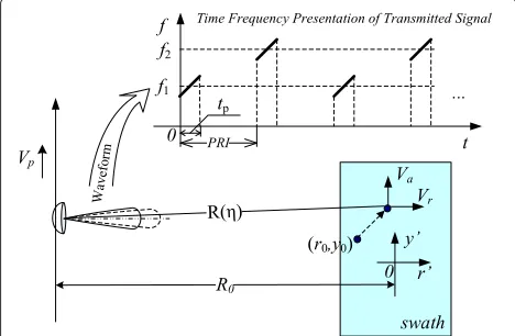
The analysis is performed in a typical slant-plane of a boresight strip-map SAR scenario shown in Figure 1. A moving target is located at (r0, y0) with respect to the scene center when it is in the antenna bore-sight direction. It moves with a constant velocityVain azimuth and a con-stant velocityVrin range. The radar platform moves with a constant velocityVp. The bore-sight distance between the radar and the scene center isR0. The time-frequency presentation of the transmitted waveform is shown at the top-right corner. The waveform consists of two kinds of pulses with the same chirp rate and pulse widthtp, but modulated by two different carrier frequencies, i.e.,f1and f2shown in the figure. The two carrier frequencies satisfy
the relationshipBp < f2−f1 f1andf1 Bp, where Bpis the bandwidth of transmitted signal. The two pulses are transmitted alternately by the same pulse repetition interval (PRI). For convenience, the two pulse bursts are denoted by c1and c2, respectively.
The slow time is denoted byη, and whenη = 0, the scene center is in the antenna bore-sight direction. The distance between the platform and the moving target is a function ofηexpressed by
R(η) =
(R0+Vrη)2+
(Vp−Va)η+y0 2
≈ R0+Vrη+
(Vp−Va)η+y0 2
2R0
. (1)
The demodulated return is
sRx(t,η)=e−j2πfct0sTx(t−t0)rect
t−t0 tp
, (2)
wheret0=2R(η)/c,cis the light speed,tis the fast time, and the function rect(t)is defined by
rect(t)=
1, |t|0.5 0, otherwise .
As we can see from (2) that the pulse compression in fast time domain does not influence the coefficiente−j2πfct0, the azimuth signal history.
Suppose that θB is the antenna beam-width, the syn-thetic aperture length will beLs = θBR0. According to kinetics theory, the synthetic aperture time is
Ts=
θBR0 Vp−Va
. (3)
So ignoring the antenna beam-pattern and the constant term, the Doppler signal history of the moving target can be approximated by
sm(η;ξm)=rect
η−η0 Ts
e−j4πλVr(η−η0)ejπfdrm(η−η0)2,
(4)
where η0 = y0/Vp, fdrm = −2(Vp−Va)2/(λR0), λ is the carrier wavelength, and ξm = (r0,y0,Vr,Va) is a vector describing the parameters of the moving target. Equation (4) indicates that the Doppler history of a mov-ing target is a chirp signal centered atfdc=−2Vr/λhaving a Doppler ratefdrm. According to the matched filter theory [24], if the azimuth signal (4) is compressed by the filter
H0(fD)=ejπksf
2
D, (5)
the compressed result will be given by
scm(η) = sin
πBD
η−η0+ VVrR20 p
π
η−
η0− VVrR20 p
∗sdiff(η),
sdiff(η) = F−1fD→η
|fD|≤BD/2
e−jπ αmksfD2
(6)
for |2Vr/λ|<fPRF/4. In (5), ks=1/fdrs, and fdrs = −2V2
p/(λR0). In (6),αm=km/ks −1 is referred to as the defocus coefficient, and the symbol “∗” means the con-volution operation. It is observed that the range motion introduces a time-delay term resulting in the misplace-ment by −VrR0/Vp relative to its real azimuth position. The time duration of (6) is
ηw≈ λ 2θBVp + |
αm|R0θB
Vp
, (7)
and the corresponding azimuth smear length is
ρsmear≈ρa+ |αm|λR0 2ρa
, (8)
where ρa = λ/(2θB) is the azimuth resolution [24]. Equation (8) indicates that the image of the moving target is smeared approximately in 1+ |αm|λR0/(2ρa2)azimuth resolution cells when its azimuth returns are compressed by (5). On the contrary, if the azimuth matched filter focuses the image of the moving target ideally, the image of background will be smeared by the same length as ρsmear.
Symmetric defocusing
As the azimuth signal history takes the form
sa(η)=ejπf
m
drη2, (9)
and according to the stationary phase theory [24], its Fourier transform is
Sa(fD,αm)=e−jπks(1+αm)f
2
D, (10)
if the azimuth signal, expressed by (9) or (10), is com-pressed by
H(fD,α)=ejπks(1+α)f
2
D, (11)
then the image of the moving target will be smeared in
M(α,αm)=1+ |α−αm|λR0 2ρ2 a
(12)
|b|2 is located in the scene and defocused by (11), we will find that (1) if the target is stationary, then its image will be smeared inM(α, 0)resolution cells and the entire sharpness becomes |b|4/M(α, 0), and that (2) if the tar-get is a moving tartar-get characterized byξm, its image will be smeared in M(α,αm) resolution cells and the entire sharpness becomes |b|4/M(α,αm). The combination of H(fD,α)andH(fD,−α)is defined as an SDFP. Inspired by the discussion above, an SDFP based MTD is described as follows.
First, the original SAR imagery is transformed to range Doppler domain and filtered by an SDFP, resulting in two defocused images. Second, the sharpness distribution images (SDI) of a defocused image are computed by
S(i,j)=
(i+1)P/2
p=(i−1)P/2+1
(j+1)Q/2
q=(j−1)Q/2+1
|I(p,q)|4, (13)
where K is the pixels number in range andL is that in azimuth of the SAR imagery,Pis the pixels in range and
Qis that in azimuth of a patch,I(p,q)is the amplitude of the (p,q)-thpixel in the defocused image, 1iM, 1jN,M = 2K/P , andN = 2L/Q . Finally, the moving targets are indicated by comparing the two SDIs.
Range velocity estimator Baseband Doppler centroid indicator
Figure 2 presents a sketch of the Doppler spectrum in the r-th range bin of the two patches containing the same moving target. The solid curve A1(fD,r) presents the Doppler spectrum of the patch from the original SAR imagery generated byc1, andA2(fD,r)presents that of the patch from that byc2. AfterA(fD,r)is normalized by
¯
A(fD,r)=
BDA(fD,r) BD/2
−BD/2A(f,r)df
, (14)
the normalized Doppler spectrum difference
Cr(fD)=
fD+f/2
fD−f/2 A¯1(f,r)− ¯A2(f,r)df
fD+f/2
fD−f/2
¯
A1(f,r)+ ¯A2(f,r)
df
(15)
Figure 2A sketch of Doppler amplitude spectra.
is chosen as the baseband Doppler centroid indicator. In (15),f = BD/N, andNis an arbitrary integer larger than 40 to our simulation experience.
It is apparent that 0 Cr(fD) 1, and the criterion amplifies the weak Doppler spectrum of moving target and suppresses the strong Doppler spectrum of back-ground. It is an important tool to analyze the Doppler centroid in this research. A typical criterion curve is shown in Figure 3. It can be seen that the two base-band Doppler centroid can be determined easily by this feature value.
Doppler ambiguity solver
The Doppler shifts of a moving target corresponding to the two carriers can be expressed by
fd1 = fdc1+m·fPRF/2= − 2Vr
λ1 , (16)
fd2 = fdc2+n·fPRF/2= − 2Vr
λ2
, (17)
wheremandnare the Doppler ambiguity numbers,λ1is the wavelength of c1, andλ2is that of c2. So the Doppler ambiguity solver is modeled by
ˆ
m,ntˆ = arg min
m,n λ1fdc1−λ2fdc2
+fPRF
2 (λ1m−λ2n)
,
(18)
s.t.
m,n∈Z,λ1> λ2 |m| 4VR
λ1fPRF,|n|
4VR
λ2fPRF
with VR being the possible maximum velocity in range. For example, on the freeway in China,VRis no more than 35 m/s, while in urban,VRwill be set to 14 m/s.
Ifmˆ andnˆare obtained from (18), then the Doppler shift can be estimated without ambiguity, and thus the range velocity can be estimated accurately.
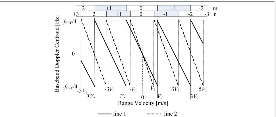
Figure 4 presents the relationship between the baseband Doppler centroid and the range velocity for the two differ-ent carriers. The horizontal axis denotes the range velocity with V1 = λ1fPRF/4 andV2 = λ2fPRF/4, and the verti-cal axis denotes the baseband Doppler centroid. Line 1
Figure 4Baseband Doppler centroid as a function of range velocity for the two carriers.
represents the baseband Doppler centroid as a function of the range velocity for c1, and line 2 represents that for c2. The integers in the upper text boxes are the ambiguity numbers, i.e.,mandnin (16) and (17), in different range velocity intervals. For a given baseband Doppler centroid
fdc, it corresponds to many different Doppler shift val-ues. If bothfdc1andfdc2are estimated, thenmandnare determined accordingly.
Algorithm 1 presents pseudo-code for the function DAS which implements Doppler ambiguity solver asso-ciated with (18). It takes as input fdc1, fdc2, f1, f2, and fPRF, and returns mˆ, nˆ. It starts by calculating the max-imum ambiguity number M and N with respect to f1 andf2with possible maximum range velocity, then com-putes fd1 and corresponding fd20 using a probing ambi-guity number m from −M to M with an increment of 1, therefore the Doppler shift difference, i.e., fm,n, is obtained by|fd2 −fd20|, wherefd2 is computed by using a probing ambiguity number nfrom −N to N with an increment of 1. Finally, the ambiguity number mˆ and nˆ
are achieved and returned by finding the minimum value offm,n.
Algorithm 1 Procedure for Doppler ambiguity solver Function [mˆ,nˆ] := DAS(fdc1,fdc2,f1,f2,fPRF)
Initialization:VR:= possible maximum range velocity;
1: λ1 := fc 1,λ2 :=
c
f2, withc being the light speed;
fd1M := 2VR
λ1 ,f
M d2 :=
2VR
λ2 ;
M := 2fd1M
fPRF,N :=
2fd2M fPRF;
2: form: = -M to M (with an increment of 1) fd1: = fdc1+m·fPRF/2;Vr: = -λ1fd1/2;fd20 := -2Vλ2r;
3: for n : = -N to N (with an increment of 1)
fd2:=fdc2+n·fPRF/2;
fm,n=fd20 −fd2; end for [n];
end for [m];
4: Find the minimum value fromfm,n
, and get the corresponding indexmˆ andnˆ;
Stepped approximation-and-comparison algorithm From Figure 4, we see that a target which moves at low speed in range direction may result in the superposition between the Doppler spectrum of background and that of the moving target. It will lead to the wrong determi-nation of Doppler spectrum peak locations. On the other hand, the estimate offdc1andfdc2may become inaccurate because of noise, platform turbulence, and clutter etc. An algorithm named SAC is developed to get a finer baseband Doppler centroid.
If the coarse baseband Doppler centroid values arefdc1 andfdc2, and the Doppler ambiguity numbersmˆ andnˆare obtained from (18), then the unambiguous Doppler shifts can be described by
fd1 = fdc1+fd+ ˆm fPRF
2 , (19)
fd2 = fdc2−fd+ ˆn fPRF
2 , (20)
wherefdis a modified Doppler shift value derived from
fˆd= arg min
fd
λ1fdc1−λ2fdc2+ fPRF
2 (λ1mˆ −λ2nˆ)
+(λ1+λ2)fd
s.t.
fd BD
2 .
Algorithm 1 presents the computation procedure of accurate fdc1 and fdc2. It takes as input fdc1, fdc2, mˆ, nˆ, fPRF,f1, andf2, wheremˆ andnˆare the ambiguity numbers computed by DAS, and returns two finer unambiguous Doppler shifts of the moving target. It starts by defining an approximation stepf=BD/(2K), whereK is an arbi-trary integer (here we assume that K is equal to 100), and computes the initial unambiguous shiftsfd10 andfd20, respectively. Then for a givenkfrom−KtoKwith incre-ment of 1, the new fd1 and fd2 are updated using (19) and (20) with the substitution ofkf tofd, and thus two corresponding range velocities resulting from the updated unambiguous Doppler shift are achieved and the differ-ence between the two velocities is stored in the sequdiffer-ence {Vk}. Finally, by searching the minimum value of{Vk}, the finer unambiguous Doppler shifts are obtained and returned.
Algorithm 2 Procedure for stepped approximation-and-comparison algorithm
Function [fˆdc1,fˆdc2] := SAC(fdc1,fdc2,mˆ,nˆ,fPRF,f1,f2) Initialization:K:= An integer larger than 100;
1: λ1= fc 1,λ2=
c f2;
fd10 :=mˆ ·fPRF/2+fdc1,fd20 :=nˆ·fPRF/2+fdc2,f :=B2KD; 2: fork:= -KtoK (with an increment of 1)
fd1:=fd10 +k·f,fd2:=fd20 −k·f; Vr1:= -λ12fd1,Vr2:= -λ22fd2;
Vk:=|Vr1−Vr2|; end for [k]
3: Find the minimum value from{Vk}, and get the modified indexk;
4: fˆdc1:=fd10 +kf,fˆdc2:=fd20 −kf;
When the finer Doppler shiftfˆd1andfˆd2are achieved, two estimates of the range velocity are computed from
ˆ
Vr1 = −
λ1fˆd1
2 , (22)
ˆ
Vr2 = −
λ2fˆd2
2 . (23)
Finally the average range velocity component is
ˆ Vr =
ˆ Vr1+ ˆVr2
2 . (24)
Further discussion
The primary condition for DAS and SAC is that the Doppler bandwidth is far smaller than fPRF (at least no more thanfPRF/4). Under this condition, iffd1andfd2are
confined by
k1 fPRF
2 −
BD
2 <fd1<k1
fPRF
2 +
BD
2 , (25)
k2 fPRF
2 −
BD
2 <fd2<k2
fPRF
2 +
BD
2 , (26)
where k1 and k2 are integers, two cases will appear in general:
Both k1and k2are equal to zero
In this case, the peaks will disappear in Cr(fd), so the range velocity component cannot be measured, thus the minimum measurable range velocity is
|Vmin,r| =λ2 BD
4 , forλ1> λ2 (27)
Either of k1and k2is not equal to zero
Ifk1=0, andfd1satisfies (25), thenfd1is
fd1=k1 fPRF
2 +δfd, (28)
where|δfd|<BD/2.fd2can be expressed by
fd2=
λ1
λ2k1
fPRF 2 +
λ1
λ2δfd. (29)
Iffd1andfd2are wrapped by the same ambiguity num-ber, thenλ1andλ2have the relationship
λ1
λ2
M+1
M , (30)
where M is the maximum ambiguity number describe in Algorithm 1. To make fdc2 detectable, the following requirement should be satisfied
λ1 λ2 −
1 fPRF 2 + λ1 λ2
δfd BD
2 . (31)
Soλ1andλ2satisfy
λ1 λ2
1+ BD
fPRF
. (32)
Equation (32) tells us that when the dual-frequency SAR system parameters, such as carrier frequencies, PRF, radar velocity and azimuth resolution, satisfy both (30) and (32), the range velocity component of a moving target can be computed without unambiguity.
Iffdc2is determined, then the ambiguity numbersmˆ and ˆ
ncan be computed from
ˆ
m,nˆ= arg min m,n
λ2fdc2+(λ2n−λ1m) fPRF
2
. (33)
In a similar way, whenk2 = 0 andfd2satisfy (26), the ambiguity numbersmˆ andnˆcan be deduced from
ˆ
m,nˆ= arg min m,n
λ1fdc1+(λ1m−λ2n) fPRF
2
Azimuth displacement correction
It is noteworthy that (6) is established based on the con-dition that|Vr/λ| < fPRF/4, and the moving target will be displaced by−VrR0/Vpin azimuth direction. It seems that the azimuth displacement is independent of the car-rier frequency. However, when the target is moving so fast that|Vr/λ| > fPRF/4, the displacement equation must be modified.
Ignoring the azimuth velocity component, the baseband Doppler history will be
φ (η)= −4π
λ R0−2π
2Vr
λ +n
fPRF 2
η−2πV
2 p
λR0
η2,
(35)
wherenis the ambiguity number of the Doppler shiftfd= −2Vr/λ. The azimuth displacement will be given by
a= −4Vr+nλfPRF
4Vp
R0. (36)
We see that if the Doppler ambiguity appears, the azimuth displacement of a moving target must be modi-fied by (36). This equation is an extension to [25,26] and is the basic model for correcting the target’s real azimuth position in a SAR image.
Azimuth velocity estimator Theoretical analysis
When a patch containing a moving target is defocused by H(fD,α) and H(fD,−α), two derivative SAR image patches, denoted byP1 andP2, are achieved simultane-ously. LetVa be an arbitrary probing azimuth velocity, and in general bothVaandVaare far less thanVp, which means thatα≈2Va/Vp. Equation (12) can be rewritten by
M(Va,Va)=1+ |
Va−Va| Vp
λR0
ρ2 a
. (37)
For simplicity, we assume that the patch contains a mov-ing point target and a stationary point target, and the two targets have the intensity|b|2 and|g|2, respectively. The patch P1has the sharpness
Sp1= |
b|4 M(Va,Va) +
|g|4 M(Va, 0)
, (38)
and P2has the sharpness
Sp2= |
b|4 M(−Va,Va)+
|g|4 M(Va, 0)
. (39)
The sharpness difference betweenSp1andSp2
f(Va)= |
b|4 M(Va,Va)−
|b|4 M(−Va,Va)
(40)
will be used as a feature to estimate the azimuth velocity component. The feature value is robust because it tries to alleviate the influence of clutters and interferences.
Let’s discuss (40). Allowing for the symmetry of the SDFP, the probing velocity Va is set to be larger than zero. ForVa > 0, 1) in the case of 0 < Va Va, the differential off(Va)is
df(Va)
dVa =
2λR0Vpρa2|b|4[(Vpρa2+λR0Va)2+(λR0Va)2]
(Vpρa2+λR0Va)2−(λR0Va)22
>0.
(41)
And 2) in the case of Va > Va, the differential of f(Va)is
df(Va) dVa =−
4λ2R20VaVpρa2|b|4(Vpρa2+λR0Va)
(Vpρa2+λR0Va)2−(λR0Va)22
<0.
(42)
The two cases show that (1) when 0 < Va Va, the sharpness difference is a monotonic increasing func-tion and it reaches the maximum value at the point where Va= Va, and (2) whenVa>Va, the sharpness differ-ence is a monotonic decreasing function and it reaches the maximum value at the point whereVa=Va. In addition, it infinitely approaches zero with the increment ofVa.
In the case of Va < 0, the following conclusions can be drawn: (1) when 0< Va−Va, the sharpness dif-ference is a monotonic decreasing function and it reaches the minimum value at the point where Va = −Va, and (2) whenVa>−Va, the sharpness difference is a monotonic increasing function and it reaches the mini-mum value at the point whereVa=Va. In addition, it infinitely approaches zero with the decrement ofVa.
Figure 5 presents a sketch of f(Va) for two cases: Va1 > 0 (for target 1) andVa2 < 0 (for target 2). We see that the maximum sharpness difference is located at the point whereVa= |Va|. If the maximum sharpness dif-ference is less than zero, then the corresponding target is moving in the opposite direction of the platform. If the maximum sharpness difference is larger than zero, then the target is moving in the direction of the platform.
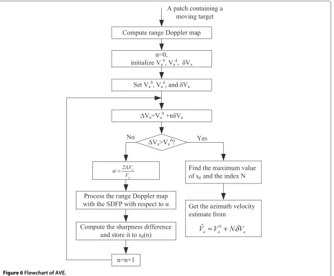
Implementation
From the discussions above, the azimuth velocity estima-tor can be modeled by
ˆ
Va= arg max
Va
f(Va). (43)
Figure 5A sketch of sharpness difference as functions ofVa.
is established to defocus the range Doppler map result-ing in two defocused images, and the sharpness difference between the two images is sent to an array named sd. The azimuth velocity estimate will appear at the position wheresdreaches the peak.
Two patches containing the same target are isolated from the two original SAR images and processed by the AVE. If the two estimates of the azimuth velocity compo-nent are denoted byVˆa1andVˆa2, then the final azimuth velocity value is synthesized by
ˆ Va=
ˆ
Va1+ ˆVa2
2 . (44)
Discussion
Let us discuss the minimum detectable azimuth velocity componentVmin,a. It is relative to the threshold valuefth which is used to identify the moving target area. We select
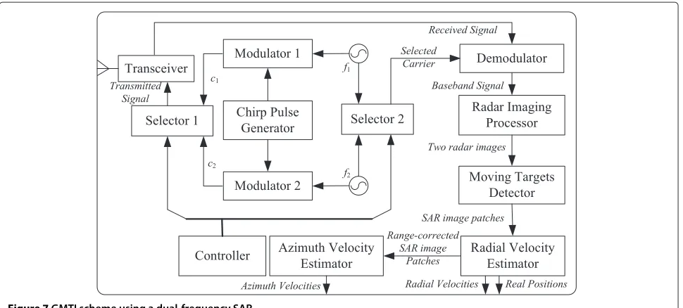
Figure 7GMTI scheme using a dual-frequency SAR.
this value according to false-alarm probabilities and detec-tion probability specificadetec-tion. According to our experience and simulation results, the feature valuef(i,j) follows a half positive Gaussian distribution approximately
p(f)= √2 2π σe
−f2
2σ2, f 0 (45)
So, from
PF= 2 √
2π σ
∞
fth
e− f2
2σ2df =erfc
fth √
2σ
(46)
we see that if a constant false alarm ratioPFis given, the threshold valuefthcan be determined.
We estimate the unknown parameter σ of (45) using MATLAB’sfminsearchroutine, which uses the Nelder-Mead parameter search procedure [27,28]. AsVmin,a Vp, we haveαmin≈2Vmin,a/Vp. Letfmaxdenote the sharp-ness of the ideally focused target, and the sharpsharp-ness of a moving target with azimuth velocityVmin,awill be
fmin,a= fmax 1+ αmλR0
ρ2 a
(47)
in the SAR image having focused background. Asfmin,a fth,αminapproximately satisfies
1− 1
1+αminλR0
ρ2
a
fth fmax
. (48)
As a result, the minimum detectable azimuth velocity is approximately
Vmin,a≈
ρa2Vp 2(1−)λR0
, (49)
where=fth/fmax.
Experiments Framework
Based on the discussions above, a sketch of the proposed single antenna SAR using a dual frequency chirp wave-form and the corresponding GMTI procedure is shown in Figure 7. In this figure, the controller controls the selec-tor 1 to pass the two kinds of pulses to the transceiver alternately, and controls the selector 2 to pass the carrier being used to the demodulators to get the corresponding baseband returns. The radar imaging processor processes the returns and generates two original SAR images. The bottom-right of the figure shows the GMTI flowchart. First, the two original SAR images are processed by the MTD, and as a result, image patches that contain the detected moving targets are achieved. Second, the isolated patches are transmitted to the RVE to estimate their range velocity components and their real azimuth positions. Finally, the range-velocity-compensated patches are sent to the AVE to estimate their azimuth velocity components.
Table 1 System parameters of field data and simulation
Symbol Description Value
Field data Simulation
R0 Range to scene center 40800 m 10000 m
Vp Platform velocity 218 m/s 200 m/s
Tp Pulse width 20μs 10μs
fp PRF 1200 Hz 4000 Hz
fc Carrier frequency 9.6 GHz 10 GHz, 12 GHz
Bw Signal bandwidth 400 MHz 200 MHz
ρr Range resolution 0.5 m 1.0 m
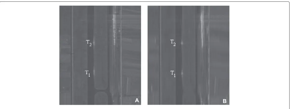
Figure 8A field SAR image containing two moving vehicles(A)and its refocused image(B).
As a result, the range and azimuth velocity components together with their real azimuth positions are worked out. We use a patch of real complex-valued SAR image to verify the MTD and AVE algorithms. The image is achieved by using one carrier, so it is cannot be used to determine the range velocity component of a moving tar-get. In order to evaluate the performance of the RVE, with no field data available so far, computer simulations are conducted to confirm the effectiveness of the proposed algorithms. The raw data are simulated by using the model proposed in [29]. The model can simulate the effects of moving targets, and it is both analytically and quantita-tively validated. We think that the following simulation based on this model can validate our idea.
AVE verification with field data
The complex-valued SAR image is collected near an air-port in Shaanxi, China. The radar system and geometry parameters are shown in Table 1. In the illuminated scene, the trajectory of the SAR is parallel to the runway, and two vehicles are running at the speed of about 5.0 m/s along the runway successively.
We isolated a patch of size 6528 pixels in range by 5120 pixels in azimuth near the moving targets from the given image. The patch is shown in Figure 8A. In this figure, the scene is about 765 m in azimuth and 600 m in range. The two known vehicles are labeled by T1and T2. We see that the background is focused fairly well while the image of the two targets are smeared.
We defocused the patch by using an SDFP with α = 0.0985 (correspondingly,Va=10 m/s). The moving tar-gets are detected correctly. An SDFP bank is constructed to estimate the azimuth velocity components of the two vehicles. In the experiment, Va ranges from 0 m/s to 30 m/s with an increment of 0.1 m/s. The range velocity components are assumed to be 0 m/s. Figure 9 presents
the normalized feature curves for T1 and T2. From the figure, the azimuth velocity estimates are −4.8 m/s and −5.0 m/s, respectively.
We refocused the moving target based on the two azimuth velocity component estimates. The result is shown in Figure 8B. It shows that the two vehicles are focused well while the background is smeared.
Performance evaluation by computer simulation
In the simulation, the background is a patch of terrain selected near the Kun-yu mountain in Shandong, China. It is about 200 m in azimuth and 160 m in range. The most important properties of the dual-frequency SAR, the moving targets and the background are incorporated. The radar system and geometry parameters are presented in Table 1.
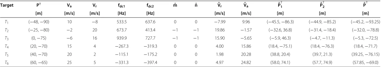
The parameters of six moving targets labeled by T1 ∼ T6 are shown in the columnsP†,Va, andVr of Table 2.
0 5 10 15 20 25 30
−1 −0.8 −0.6 −0.4 −0.2 0 0.2 0.4
ΔVa [m/s]
Normalized Sharpness Difference
T1
T2
Journal
o
n
A
dvances
in
Signal
Processing
2012,
2012
:236
Page
11
of
14
Table 2 Moving target parameters and their estimated results
Target P† V
a Vr fdc1 fdc2 mˆ nˆ Vˆr Vˆa Pˆ
†
1 Pˆ
†
2 Pˆ
†
[m] [m/s] [m/s] [Hz] [Hz] [m/s] [m/s] [m] [m] [m]
T1 (−48,−90) 10 −8 533.5 637.6 0 0 −7.99 9.96 (−45.5,−86.3) (−44.9,−85.2) (−45.2,−93.25)
T2 (−25,−80) −2 20 673.7 413.4 −1 −1 19.86 −1.57 (−32.6, 36.8) (−31.4,−18.4) (−32.0,−78.8)
T3 (0,−75) −6 16 939.9 727.7 −1 −1 15.90 −5.65 (−5.9, 46.3) (−4.7,−11.3) (−5.3,−72.5)
T4 (20,−70) 15 4 −267.3 −319.3 0 0 4.00 15.86 (18.4,−75.1) (18.4,−76.3) (18.4,−71.7)
T5 (40,−70) 20 2 −115.1 −175.2 0 0 1.98 20.28 (38.8, 20.4) (39.7, 21.3) (39.25,−76.15)
T6 (60,−65) 25 5 −331.3 −397.4 0 0 4.97 24.82 (58.0, 74.1) (57.7, 74.9) (57.85,−69.0)
†P denotes the real position of the targets whenη=0.Pˆ
Figure 10Computer simulated SAR images for 10 GHz(A)and 12 GHz(B).
The customized target size is 3 m in azimuth by 5 m in range with the average back reflective coefficient of the simulated scene. The targets are arranged to move on a road in the selected scene.
Figure 10A,B present two simulated SAR images gen-erated by c1and c2, respectively. In the two images, the background is well focused while the moving targets are
smeared due to their motions. We defocused the images by using SDFPs corresponding toVa =5 m/s, 10 m/s, and 20 m/s. As a result, the moving targets are detected correctly.
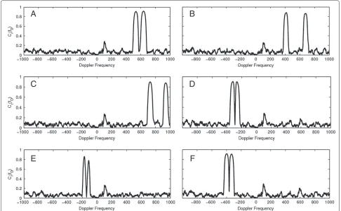
The detected moving targets are isolated from the two original SAR images and the normalized Doppler differ-ence curves of T1 ∼ T6 are computed. The results are
B
A
D
C
F
E
Figure 11Normalized Doppler difference curves of six simulated moving targets.(A)presents the normalized Doppler difference of target T1,
presented in Figure 11A–F, respectively. The peak loca-tions are listed in the columnsfdc1andfdc2of Table 2. The Doppler ambiguity is solved by the DAS algorithm and shown in the column ofmˆ andnˆ. The final range velocity components are computed by using the SAC algorithm. The results are listed in the columnVˆrof Table 2. The esti-mated target positions are presented in the columnsPˆ1,
ˆ
P2, andPˆ of Table 2. The data in Table 2 confirm that the proposed DAS and SAC algorithms works well.
The detected targets are compensated by the range velocity estimates, and then the azimuth velocity compo-nents are computed then by constructing an SDFP bank withVaranging from 0 to 30 m/s increased by the step 0.02 m/s. The sharpness difference curves of the mov-ing targets have the same profiles as that presented in Figure 9. The estimated results are shown in the column
ˆ
Va of Table 2. The results show that the estimate is not accurate when the azimuth velocity is less than 2 m/s. One principal reason lies in that the image of the moving target may be smeared slightly and thus the corresponding fea-ture curve becomes so flat that the peak may appear at the position far from the real velocity value.
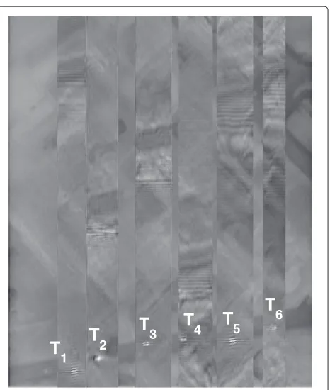
According to the estimates in the columns Vˆr andVˆa of Table 2, the moving targets are refocused and their displaced azimuth positions are corrected. Without loss of generality, Figure 10A is selected as an example to show the correction and refocusing effectiveness. For each detected moving target in the SAR image, a slice which covers all the range bins that the moving target occupies is cropped. After range velocity compensated, it is refo-cused by using an azimuth matched filter with Doppler chirp ratefˆdrm = −2(Vp− ˆVa)2/(λ1R0). All the processed slices are stitched together with the original SAR image to show the real positions of the moving targets. Figure 12 presents the stitched product. From this figure we see that the moving targets are focused well while the background in each slice is smeared. The moving targets are just at the places that listed in columnPˆ†of Table 2.
Conclusion
A scheme for velocity components estimation in GMTI is proposed based on a single antenna SAR using a dual-frequency chirp waveform. The scheme consists of a moving target detector, a range velocity estimator and an azimuth velocity estimator, and it can locate the real posi-tion of the detected moving target by using a modified azimuth displacement correction model.
The moving target detector uses an SDFP to detect the possible moving targets with a limited azimuth velocity range near a certain value in the give complex SAR image. It is proved to be effective and efficient by field and sim-ulated data. In practice, when the azimuth velocity varies widely, many SDFPs are needed to detect all the moving targets.
T
1
T
2
T
3
T
4T
5
T
6
Figure 12Refocused and azimuth-displacement-corrected moving targets.
The azimuth velocity estimator is established by using an SDFP bank. The effectiveness of the model is ver-ified by simulated and field data. The AVE is robust because it tries to alleviate the influences of the clutters and interferences.
The range velocity estimator is based on the Doppler shift information introduced by range velocity compo-nent. Two algorithms, DAS and SAC, are designed to solve the Doppler ambiguity and make the Doppler cen-troid estimation more accurate. For each pulse burst, the baseband Doppler centroid is estimated by using a cri-terion named normalized Doppler spectrum difference. In addition, traditional azimuth displacement equation is modified to get the correct azimuth position of a moving target. Simulation results validate the improvement.
Competing interests
The authors declare that they have no competing interests.
Acknowledgments
We appreciate the support from the National Science Foundation of China (Grant Number: 61072150) and the National Basic Research Program of China (Grant Numbers: 2009CB824903 and 2010CB731904).
Received: 27 February 2012 Accepted: 25 September 2012 Published: 12 November 2012
References
2. D Vu, B Guo, L Xu, J Li, inAlgorithms for Synthetic Aperture Radar Imagery XVI, Proceedings of the SPIE. SAR based adaptive GMTI (vol. 7699, 76990H–76990H-12, Bellingham, WA, USA, 2010)
3. D Cerutti-Maori, CH Gierull, J Ender, Experimental verificaiton of SAR-GMTI improvement through antenna switching. IEEE Trans. Geosci. Rem. Sens. 48(4), 2066–2075 (2010)
4. CH Gierull, Ground moving target parameter estimation for two-channel SAR. IET-Radar Sonar Navig.153(3), 224–233 (2006)
5. G Krieger, N Gebert, A Moreira, Multidimensional waveform encoding: a new digital beamforming technique for synthetic aperture radar remote sensing. IEEE Trans. Geosci. Rem. Sens.46, 31–46 (2008)
6. SK Wong, High range resolution profiles as motion-invariant features for moving ground targets identification in SAR-based automatic target recognition. IEEE Trans. Aerosp. Electron. Syst.45(3), 1017–1039 (2009) 7. M Gisself¨alt, T Pernst˚al, inProceedings of IEEE Radar Conference, vol. 2010.
STAP analysis using multi-channel airborne radar data from flight trials (USA, Washington, DC, 2010), pp. 407–411
8. S Chiu, MV Dragoˇsevi´c, Moving target indication via RADARSAT-II multichannel synthetic aperture radar processing. EURASIP J. Adv. Signal Process.2010(Article ID 740130), 1–19 (2010)
9. S Zhu, G Liao, Y Qu, Z Zhou, X Liu, Ground moving targets imaging algorithm for synthetic aperture radar. IEEE Trans. Geosci. Rem. Sens.49, 462–477 (2011)
10. DM Vavriv, OO Bezvesilniy, inProceedings of RAST, vol. 2011. Potential of multi-look SAR processing (Istanbul, Turkey, 2011), pp. 365–369 11. JR Fienup, Detecting moving targets in SAR imagery by focusing. IEEE
Trans. Aerosp. Electron. Syst.37(3), 794–809 (2001)
12. PAC Marques, JMB Dias, Moving targets processing in SAR spatial domain. IEEE Trans. Aerosp. Electron. Syst.43(3), 864–874 (2007)
13. S Hinz, F Meyer, A Laika, R Bamler, inProceedings of IEEE computer society conference CVPR. Spaceborne traffic monitoring with dual channel synthetic aperture radar-theory and experiments, vol. 13, 1063-6919/05 (San Diego, CA, USA, 2005). pp.1–7
14. DA Cook, DC Brown, Analysis of phase error effects on stripmap SAS. IEEE J. Ocean. Eng.34(3), 250–261 (2009)
15. SV Baumgartner, G Krieger, Accleration-independent along-track velocity estimaiton of moving targets. IET-Radar Sonar Navig.4(3), 474–487 (2009) 16. CY Chang, JC Curlander, Application of the multiple PRF technique to
resolve Doppler centroid estimation ambiguity for spaceborne SAR. IEEE Trans. Geosci. Rem. Sens.30(5), 941–949 (1992)
17. R Bamler, H Runge, P R F ambiguity resolving by wavelength diversity. IEEE Trans. Geosci. Rem. Sens.29(6), 997–1003 (1991)
18. FH Wong, IG Cumming, A combined SAR Doppler centroid estimation scheme based upon signal phase. IEEE Trans. Geosci. Rem. Sens.34(3), 696–717 (1996)
19. SN Madsen, Estimating the Doppler centroid of SAR data. IEEE Trans. Aerosp. Electron. Syst.25(2), 134–140 (1989)
20. R Bamler, Doppler frequency estimation and the Cramer-Rao bound. IEEE Trans. Geosci. Rem. Sens.29(3), 385–390 (1991)
21. JR Moreira, A new method of aircraft motion error extraction from radar raw data for real time motion compensation. IEEE Trans. Geosci. Rem. Sens.28(4), 620–626 (1990)
22. JR Moreira, W Keydel, A new MTI-SAR approach using the reflectivity displacement method. IEEE Trans. Geosci. Rem. Sens.33(5), 1238–1244 (1995)
23. J Wang, X Liu, inProceedings of IEEE IGARSS, vol. 2011. Velocity estimation of moving targets using SAR (Vancouver, Canada, 2011), pp. 340–343 24. BC Wang,Digital Signal Processing Techniques and Applications in Radar
Image Processing. (John Wiely and Sons Inc., Hoboken, 2008) 25. M R ¨uegg, E Meier, D N ¨uesch, Capabilities of dual-frequency millimeter
wave SAR with monopulse processing for ground moving target indication. IEEE Trans. Geosci. Rem. Sens.45(3), 539–553 (2007) 26. RK Raney, Synthetic aperture imaging radar and moving targets. IEEE
Trans. Aerosp. Electron. Syst.AES-7(3), 499–505 (1971)
27. IG Cumming, S Li, Improved slope estimation for SAR Doppler ambiguity resolution. IEEE Trans. Geosci. Rem. Sens.44(3), 707–718 (2006) 28. JC Lagarias, JA Reeds, MH Wright, PE Wright, Convergence properties of
the Nelder-Mead simplex method in low dimensions. SIAM J. Optim.9, 112–147 (1998)
29. O Dogan, M Kartal, Efficient strip-mode SAR raw-data simulation of fixed and moving targets. IEEE Geosci. Rem. Sens. Lett.8(5), 884–888 (2011)
doi:10.1186/1687-6180-2012-236
Cite this article as:Lvet al.:Ground moving target indication and param-eters estimation using a dual-frequency synthetic aperture radar.EURASIP Journal on Advances in Signal Processing20122012:236.
Submit your manuscript to a
journal and benefi t from:
7Convenient online submission
7Rigorous peer review
7Immediate publication on acceptance
7Open access: articles freely available online
7High visibility within the fi eld
7Retaining the copyright to your article