doi:10.1155/2009/968345
Research Article
Combination of Adaptive Feedback Cancellation and Binaural
Adaptive Filtering in Hearing Aids
Anthony Lombard, Klaus Reindl, and Walter Kellermann
Multimedia Communications and Signal Processing, University of Erlangen-Nuremberg, Cauerstr. 7, 91058 Erlangen, Germany
Correspondence should be addressed to Anthony Lombard,[email protected]
Received 12 December 2008; Accepted 17 March 2009
Recommended by Sven Nordholm
We study a system combining adaptive feedback cancellation and adaptive filtering connecting inputs from both ears for signal enhancement in hearing aids. For the first time, such a binaural system is analyzed in terms of system stability, convergence of the algorithms, and possible interaction effects. As major outcomes of this study, a new stability condition adapted to the considered binaural scenario is presented, some already existing and commonly used feedback cancellation performance measures for the unilateral case are adapted to the binaural case, and possible interaction effects between the algorithms are identified. For illustration purposes, a blind source separation algorithm has been chosen as an example for adaptive binaural spatial filtering. Experimental results for binaural hearing aids confirm the theoretical findings and the validity of the new measures.
Copyright © 2009 Anthony Lombard et al. This is an open access article distributed under the Creative Commons Attribution License, which permits unrestricted use, distribution, and reproduction in any medium, provided the original work is properly cited.
1. Introduction
Traditionally, signal enhancement techniques for hearing aids (HAs) were mainly developed independently for each ear [1–4]. However, since the human auditory system is a binaural system combining the signals received from both ears for audio perception, providing merely bilateral systems (that operate independently for each ear) to the hearing-aid user may distort crucial binaural information needed to localize sound sources correctly and to improve speech perception in noise. Foreseeing the availability of wireless technologies for connecting the two ears, several binaural processing strategies have therefore been presented in the last decade [5–10]. In [5], a binaural adaptive noise reduction algorithm exploiting one microphone signal from each ear has been proposed. Interaural time difference cues of speech signals were preserved by processing only the high-frequency components while leaving the low frequencies unchanged. Binaural spectral subtraction is proposed in [6]. It utilizes cross-correlation analysis of the two microphone signals for a more reliable estimation of the common noise power spectrum, without requiring stationarity for the interfering noise as the single-microphone versions do. Binaural multi-channel Wiener filtering approaches preserving binaural
cues were also proposed, for example, in [7–9], and signal enhancement techniques based on blind source separation (BSS) were presented in [10].
Research on feedback suppression and control system theory in general has also given rise to numerous hearing-aid specific publications in recent years. The behavior of unilateral closed-loop systems and the ability of adaptive feedback cancellation algorithms to compensate for the feedback has been extensively studied in the literature (see, e.g., [11–15]). But despite the progress in binaural signal enhancement, binaural systems have not been considered in this context. In this paper, we therefore present a theoretical analysis of a binaural system combining adaptive feedback cancellation (AFC) and binaural adaptive filtering (BAF) techniques for signal enhancement in hearing aids.
The paper is organized as follows. An efficient binaural configuration combining AFC and BAF is described in
in Section 4. Here, to illustrate our argumentation, a BSS scheme has been chosen as an example for adaptive binaural filtering. Experimental conditions and results are finally presented in Sections5and6before providing concluding remarks inSection 7.
2. Signal Model
AFC and BAF techniques can be combined in two different ways. The feedback cancellation can be performed directly on the microphone inputs, or it can be applied at a later stage, to the BAF outputs. The second variant requires in general fewer filters but it has also several drawbacks. Actually, when the AFC comes after the BAF in the processing chain, the feedback cancellation task is complicated by the necessity to follow the continuously time-varying BAF filters. It may also significantly increase the necessary length of the AFC filters. Moreover, the BAF cannot benefit from the feedback cancellation effectuated by the AFC in this case. Especially at high HA amplification levels, the presence of strong feedback components in the sensor inputs may, therefore, seriously disturb the functioning of the BAF. These are structurally the same effects as those encountered when combining adaptive beamforming with acoustic echo cancellation (AEC) [16].
In this paper, we will therefore concentrate on the “AFC-first” alternative, where AFC is followed by the BAF.
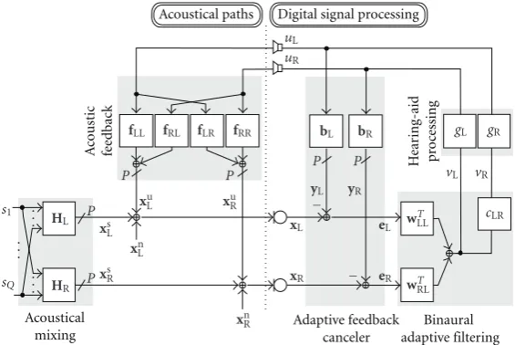
Figure 1depicts the signal model adopted in this study. Each component of the signal model will be described separately in the following and generic vector/matrix notations will be introduced to carry out a general analysis of the overall system in Sections3and4.
2.1. Notations. In this paper, lower-case boldface characters represent (row) vectors capturing signals or the filters of single-input-multiple-output (SIMO) systems. Accordingly, multiple-input-single-output (MISO) systems are described by transposed vectors. Matrices denoting multiple-input-multiple-output (MIMO) systems are represented by upper-case boldface characters. The transposition of a vector or a matrix will be denoted by the superscript{·}T
.
2.2. The Microphone Signals. We consider here multi-sensor hearing aid devices with P microphones at each ear (see
Figure 1), whereP typically ranges between one and three. Because of the reverberation in the acoustical environment,
Q point source signals sq (q = 1,. . .,Q) are filtered by a MIMO mixing system (one Q×P MIMO system for each ear in the figure) modeled by finite impulse response (FIR) filters. This can be expressed in thez-domain as:
xs Ip(z)=
Q
q=1
sq(z)hqIp(z) I∈ {L, R}, (1)
wherexs
Ip(z) is thez-domain representation of the received source signal mixture at the pth sensor of the left (I = L) and right (I = R) hearing aid, respectively. hqLp(z) and
hqRp(z) denote the transfer functions (polynomes of order up to several thousands typically) between the qth source
and the pth sensor at the left and right ears, respectively. One of the point sources may be seen as the target source to be extracted, the remaining Q−1 being considered as interfering point sources. For the sake of simplicity, thez -transform dependency (z) will be omitted in the rest of this paper, as long as the notation is not ambiguous.
The acoustic feedback originating from the loudspeakers (LS) uL and uR at the left and right ears, respectively,
is modeled by four 1 × P SIMO systems of FIR filters.
fLLp and fRLp represent the (z-domain) transfer functions (polynomes of order up to several hundreds typically) from the loudspeakers to the pth sensor on the left side, and
fLRp and fRRp represent the transfer functions from the loudspeakers to the pth sensor on the right side. The feedback components captured by the pth microphone of each ear can therefore be expressed in thez-domain as
xu
Ip=uLfLIp+uRfRIp I∈ {L, R}. (2) Note that as long as the energy of the two LS signals are comparable, the “cross” feedback signals (traveling from one ear to the other) are negligible compared to the “direct” feedback signals (occuring on each side independently). With the feedback paths (FBP) used in this study (see the description of the evaluation data inSection 5.3), an energy difference ranging from 15 to 30 dB has been observed between the “direct” and “cross” FBP impulse responses. When the HA gains are set at similar levels in both ears, the “cross” FBPs can then be neglected. But the impact of the “cross” feedback signals becomes more significant when a large difference exists between the two HA gains. Here, therefore, we explicitly account for the two types of feedback by modelling both the “direct” paths (with transfer functions
fLLp and fRRp, p = 1,. . .,P) and the “cross” paths (with
transfer functionsfRLpandfLRp,p=1,. . .,P) by FIR filters. Diffuse noise signalsnLpandnRp,p=1,. . .,Pconstitute the last microphone signal components on the left and right ears, respectively. The z-domain representation of the pth sensor signal at each ear is finally given by:
xIp=x
s Ip+x
n Ip+x
u
Ip I∈ {L, R}. (3) This can be reformulated in a compact matrix form jointly capturing thePmicrophone signals of each HA:
x=xs+xn+xu=sH+xn+uF, (4) where we have used thez-domain signal vectors
s=s1,. . .,sQ
, (5)
xsL=
xs L1,. . .,x
s LP
, (6)
xs R=
xs R1,. . .,x
s RP
, (7)
xs=xLs xsR
, (8)
u=uL uR
Acoustical paths
Acoustical mixing
Digital signal processing
A
coustic
feedback
Adaptive feedback canceler
Binaural adaptive filtering
He
a
r
in
g
-aid
pr
oc
essin
g
uL uR
fLL fRL fLR fRR bL bR gL gR
vL vR
. . . . . .
. . . s1
sQ
−
− P
P
P P P P
xuL xRu
xsL
xsR
xn R
xL
xR xnL
HL
HR
yL yR
eL
eR wTLL
wT RL
wTLR
wTRR
Figure1: Signal model of the AFC-BAF combination.
as well as thez-domain matrices
HL=
⎡ ⎢ ⎢ ⎢ ⎢ ⎣
h1L1 · · · h1LP ..
. . .. ...
hQL1 · · · hQLP ⎤ ⎥ ⎥ ⎥ ⎥
⎦, (10)
HR=
⎡ ⎢ ⎢ ⎢ ⎢ ⎣
h1R1 · · · h1RP ..
. . .. ...
hQR1 · · · hQRP ⎤ ⎥ ⎥ ⎥ ⎥
⎦, (11)
H=[HL HR], (12)
fLL=
fLL1,. . .,fLLP
, (13)
fRL=
fRL1,. . .,fRLP
, (14)
FL=
fT
LL fRLT
T
, (15)
fLR=
fLR1,. . .,fLRP
, (16)
fRR=
fRR1,. . .,fRRP
, (17)
FR=
fLRT fRRT T, (18)
F=FL FR
=
⎡
⎣fLL fLR
fRL fRR
⎤
⎦. (19)
Furthermore, xn and xu capturing the noise and feedback
components present in the microphone signals are defined in a similar way toxs. The sensor signal decomposition (4)
can be further refined by distinguishing between target and interfering sources:
xs=xstar +xsint
=starhtar+sintHint. (20)
starrefers to the target source andsintis a subset ofscapturing
theQ−1 remaining interfering sources.htaris a row of H
which captures the transfer functions from the target source to the sensors andHintis a matrix containing the remaining
Q−1 rows ofH. Like the other vectors and matrices defined above, these four entities can be further decomposed into their left and right subsets, labeled with the indices L and R, respectively.
2.3. The AFC Processing. As can be seen fromFigure 1, we apply here AFC to remove the feedback components present in the sensor signals, before passing them to the BAF. Feed-back cancellation is achieved by trying to produce replicas of these undesired components, using a set of adaptive filters. The solution adopted here consists of two 1×PSIMO systems of adaptive FIR filters, with transfer functions bLp andbRp between the left (resp. right) loudspeaker and thepth sensor on the left (resp. right) side. The output
yIp=uIbIp I∈ {L, R} (21)
of thepth filter on the left (resp. right) side is then subtracted from the pth sensor signal on the left (resp. right) side, producing a residual signal
eIp=xIp−yIp I∈ {L, R}, (22)
which is, ideally, free of any feedback components. (21) and (22) can be reformulated in matrix form as follows:
e=x−y=x−uB, (23) with the block-diagonal constraint
B=! Bc=
⎡
⎣bL 0
0 bR
⎤
put on the AFC system. The vectors e and y, capturing the z-domain representations of the residual and AFC output signals, respectively, are defined in analogous way to xs in (8). As can be seen from (21) and (22), we
perform here bilateral feedback cancellation (as opposed to binaural operations) since AFC is performed for each ear separately. This is reflected in (24), where we force the off -diagonal terms to be zero instead of reproducing the acoustic feedback system F with its set of four SIMO systems. The reason for this will become clear inSection 3.1. Guidelines regarding an arbitrary (i.e., unconstrained) AFC system B (defined similarly to F in this case) will also be provided at some points in the paper. The superscript {·}c is used
to distinguish constrained systemsBc defined by (24) from
arbitrary (unconstrained) systemsB(with possibly non-zero off-diagonal terms).
2.4. The BAF Processing. The BAF filters perform spatial filtering to enhance the signal coming from one of the Q
external point sources. This is performed here binaurally, that is, by combining signals from both ears (seeFigure 1). The binaural filtering operations can be described by a set of fourP×1 MISO systems of adaptive FIR filters. This can be expressed in thez-domain as follows:
vI=
P
p=1
eLpwLpI+eRpwRpI I∈ {L, R}, (25)
where wLpI and wRpI, p = 1,. . .,P, I ∈ {L, R} are the transfer functions applied on the pth sensor of the left and right hearing aids, respectively. To reformulate (25) in matrix form, we define the vector
v=vL vR
, (26)
which jointly captures thez-domain representations of the two BAF outputs, and the vector and matrices
wLL=
wL1L,. . .,wLPL
, (27)
wRL=
wR1L,. . .,wRPL
, (28)
wL=
wLL wRL
, (29)
wLR=
wL1R,. . .,wLPR
, (30)
wRR=
wR1R,. . .,wRPR
, (31)
wR=
wLR wRR
, (32)
W=wTL wTR
=
⎡
⎣wTLL wTLR
wTRL wRRT
⎤
⎦, (33)
related to the transfer functions of the MIMO BAF system. We can finally express (25) as:
v=e W. (34)
2.5. The Forward Paths. Conventional HA processing (mainly a gain correction) is performed on the output of the AFC-BAF combination, before being played back by the loudspeakers:
uI=vIgI I∈ {L, R}, (35)
wheregLandgRmodel the HA processing in thez-domain, at
the left and right ears, respectively. In the literature, this part of the processing chain is often referred to as the forward path (in opposition to the acoustic feedback path). To facilitate the analysis, we will assume that the HA processing is linear and time-invariant (at least between two adaptation steps) in this study. (35) can be conveniently written in matrix form as:
u=vDiagg, (36) with
g=gL gR
. (37)
The Diag{·}operator applied to a vector builds a diagonal matrix with the vector entries placed on the main diagonal.
Note that for simplicity, we assumed that the number of sensors P used on each device for digital signal processing was equal. The above notations as well as the following analysis are however readily applicable to asymmetrical con-figurations also, simply by resizing the above-defined vectors and matrices, or by setting the corresponding microphone signals and all the associated transfer functions to zero. In particular, the unilateral case can be seen as a special case of the binaural structure discussed in this paper, with one or more microphones used on one side, but none on the other side.
3. Interaction Effects on the Feedback
Cancellation
The structure depicted inFigure 1for binaural HAs mainly deviates from the well-known unilateral case by the pres-ence of binaural spatial filtering. The binaural structure is characterized by a significantly more complex closed-loop system, possibly with multiple microphone inputs, but most importantly with two connected LS outputs, which considerably complicates the analysis of the system. However, we will see in the following how, under certain conditions, we can exploit the compact matrix notations introduced in the previous section, to describe the behavior of the closed-loop system. We will draw some interesting conclusions on the present binaural system, emphasizing its deviation from the standard unilateral case in terms of ideal cancellation solution, convergence of the AFC filters and system stability.
Acoustical paths
Acoustical mixing
Digital signal processing
A
coustic
feedback
Adaptive feedback canceler
Binaural adaptive filtering
He
a
r
in
g
-aid
pr
oc
essin
g
uL uR
fLL fRL fLR fRR bL bR gL gR
vL vR
. . . . . .
. . . s1
sQ
−
− P
P
P P P P
xuL xRu
xs L
xsR
xnR xL
xR xnL
HL
HR
yL yR
eL
eR
cLR wLLT
wRLT
Figure2: Equivalent signal model of the AFC-BAF combination under the assumption (40).
[11] (the stability of the binaural closed-loop system will be discussed in Section 3.3). The adaptation of the filter coefficients towards the desired solution is usually achieved using a gradient-descent-like learning rule, in its simplest form using the least mean square (LMS) algorithm [17]. The functioning of the AFC in the binaural configuration shown inFigure 1is similar.
The residual signal vector (23) can be decomposed into its source, noise and feedback components using (4):
e=xs+xn+u(F−B)
eFB
, (38)
whereB denotes an arbitrary (unconstrained) AFC system matrix (Section 2.3).eFB=eFB
L eFBR
=[eFBL1,. . .,e
FB LP,e
FB R1,. . .,
eFB
RP] captures thez-domain representations of the residual feedback components to be removed by the AFC. The only way to perfectly remove the feedback components from the residual signals (i.e., eFB = 0), for arbitrary output signal
vectorsu, is to have
B=F= B. (39)
Bdenotes the ideal AFC solution in theunconstrainedcase. This is the binaural analogon to the ideal AFC solution in the unilateral case, where perfect cancellation is achieved by reproducing an exact replica of the acoustical FBP. In practice, this solution is however very difficult to reach adaptively because it requires the two signals uL and uR
to be uncorrelated, which is obviously not fulfilled in our binaural HA scenario since the two HAs are connected (the correlation is actually highly desirable since the HAs should form a spatial image of the acoustic scene, which implies that the two LS signals must be correlated to reflect interaural time and level differences). This problem has been extensively described in the literature on multi-channel AEC, where it is referred to as the “non-uniqueness problem”. Several attempts have been reported in the literature to partly
alleviate this issue (see, e.g., [18–20]). These techniques may be useful in the HA case also, but this is beyond the scope of the present work.
In this paper, instead of trying to solve the problem mentioned above, we explicitly account for the correlation of the two LS output signals. The relation between the HA outputs can be tracked back to the relation existing between the BAF outputsvL andvR(Figure 1), which are generated
from the same set of sensors and aim at reproducing a binaural impression of the same acoustical scene. The relation between vL and vR can be described by a linear
operatorcLR(z) transformingvL(z) intovR(z) such that:
vR=vLcLR ∀vL, (40)
which is actually perfectly true if and only ifcLRtransforms
wLintowR:
wR=wLcLR. (41)
Therefore, the assumption (40) will only be an approxima-tion in general, except for a specific class of BAF systems satisfying (41). The BSS algorithm discussed in Section 4
belongs to this class. Figure 2 shows the equivalent signal model resulting from (40). As can be seen from the figure,
cLRcan be equivalently considered as being part of the right
forward path to further simplify the analysis. Accordingly, we then define the new vector
g=gL gR
=gL cLRgR
(42)
jointly capturingcLRand the HA processing. Provided that
gLandgRare linear, (41) (and hence (40)) is equivalent to
assuming the existence of a linear dependency between the LS outputs, which we can express as follows:
u=vLg= uL
gL g=
uR
This assumption implies that only one filter (instead of two, one for each LS signal) suffices to cancel the feedback components in each sensor channel. It corresponds to the constraint (24) mentioned inSection 2.3, which forces the AFC system matrixB to be block-diagonal (B =! Bc). The
required number of AFC filters reduces accordingly from 2×2Pto 2P.
Using the constraint (24) and the assumption (43) in (38), we can derive the constrained ideal AFC solution minimizingeFBI , I∈ {L, R}, considering each side separately:
eFBI =uFI−uIbI
= uI
gI
gFI−uIbI
=uI
⎡
⎣gF IgI−1
bI
−bI
⎤
⎦ I∈ {L, R}. (44)
Here,bIdenote the ideal AFC solution for the left or right
HA. It can be easily verified that inserting (44) into (23) leads to the following residual signal decomposition:
e=xs+xn+uBc−Bc
eFB
, (45)
where
Bc= BdiagbL,bR
(46)
denotes the ideal AFC solution whenBis constrained to be block-diagonal (B =! Bc) and under the assumption (43).
The Bdiag{·}operator is the block-wise counterpart of the Diag{·} operator. Applied to a list of vectors, it builds a block-diagonal matrix with the listed vectors placed on the main diagonal of the block-matrix, respectively.
To illustrate these results, we expand the ideal AFC solution (46) using (15) and (18):
bL=
gLfLL+gRfRL
g−1 L
= fLL direct
+g R/gLfRL cross
,
bR=
gRfRR+gLfLR
g−1 R
= fRR direct
+ g R/gLfRL cross
.
(47)
For each filter, we can clearly identify two terms due to, respectively, the “direct” and “cross” FBPs (seeSection 2.2). Contrary to the “direct” terms, the “cross” terms are identifiable only under the assumption (43) that the LS outputs are linearly dependent. Should this assumption not hold because of, for example, some non-linearities in the forward paths, the “cross” FBPs would not be completely identifiable. The feedback signals propagating from one ear
to the other would then act as a disturbance to the AFC adaptation process. Note, however, that since the amplitude of the “cross” FBPs is negligible compared to the amplitude of the “direct” FBPs (Section 2.2), the consequences would be very limited as long as the HA gains are set to similar amplification levels, as can be seen from (47). It should also be noted that the forward path generally includes some (small) decorrelation delays DL and DR to help the AFC
filters to converge to their desired solution (seeSection 3.2). If those delays are set differently for each ear, causality of the “cross” terms in (47) will not always be guaranteed, in which case the ideal solution will not be achievable with the present scheme. This situation can be easily avoided by either setting the decorrelation delays DL = DR equal for
each ear (which appears to be the most reasonable choice to avoid artificial interaural time differences), or by delaying the LS signals (but using the non-delayed signals as AFC filter inputs). However, since it would further increase the overall delay from the microphone inputs to the LS outputs, the latter choice appears unattractive in the HA scenario.
3.2. The Binaural Wiener AFC Solution. In the configuration depicted in Figure 2, similar to the standard unilateral case (see, e.g., [12]), conventional gradient-descent-based learning rules do not lead to the ideal solution discussed in Section 3.1 but to the so-called Wiener solution [17]. Actually, instead of minimizing the feedback components eFBin the residual signals, the AFC filters are optimized by
minimizing the mean-squared error of the overallresidual signals (38).
In the following, we conduct therefore a convergence analysis of the binaural system depicted in Figure 2, by deriving the Wiener solution of the system in the frequency domain:
bWiener I
z=ejω=r
xIuI
ejωr−1
uIuI
ejω
=ruuIFI+rxsIuI+rxnIuI
r−1
uIuI (48)
=gF IgI−1
bI(z=ejω)
+rxs IuIr−
1
uIuI+rxnIuIr−
1
uIuI
˘
bI(z=ejω)
I∈{L, R},
(49)
where the frequency dependency (ejω) was omitted in (48) and (49) for the sake of simplicity, like in the rest of this section.bI(z=ejω) is recognized as the (frequency-domain)
ideal AFC solution discussed inSection 3.1, and ˘bI(z=ejω)
denotes a (frequency-domain) bias term. The assumption (43) has been exploited in (48) to obtain the above final result.ruIuIrepresents the (auto-) power spectral density of
uI, I ∈ {L, R}, andrxIuI = [rxI1uI,. . .,rxIPuI], I ∈ {L, R}, is a vector capturing power spectral densities. The cross-power spectral density vectorsrxs
IuIandrxnIuIare defined in a similar way.
The Wiener solution (49) shows that the optimal solution is biased due to the correlation of the different source contributionsxs and xn with the reference inputs u
I, I ∈
distinguishing between desired (target source) and undesired (interfering point sources and diffuse noise) sound sources:
˘ bWienerI
ejω= rxStar I uIr
−1
uIuI
due to target source
+ rxSint I uIr
−1
uIuI+rxInuIr
−1
uIuI
due to undesired sources
I∈ {L, R}.
(50) By nature, the spatially uncorrelated diffuse noise compo-nentsxnwill be only weakly correlated with the LS outputs.
The third bias term will have therefore only a limited impact on the convergence of the AFC filters. The diffuse noise sources will mainly act as a disturbance. Depending on the signal enhancement technique used, they might even be partly removed. But above all, the (multi-channel) BAF performs spatial filtering, which mainly affects the interfer-ing point sources. Ideally, the interferinterfer-ing sources may even vanish from the LS outputs, in which case the second bias term would simply disappear. In practice, the interference sources will never be completely removed. Hence the amount of bias introduced by the interfering sources will largely depend on the interference rejection performance of the BAF. However, like in the unilateral hearing aids, the main source of estimation errors comes from the target source. Actually, since the BAF aims at producing outputs which are as close as possible to the original target source signal, the first bias term due to the (spectrally colored) target source will be much more problematic.
One simple way to reduce the correlation between the target source and the LS outputs is to insert some delaysDL
andDRin the forward paths [12]. The benefit of this method
is however very limited in the HA scenario where only tiny processing delays (5 to 10 ms for moderate hearing losses) are allowed to avoid noticeable effects due to unprocessed signals leaking into the ear canal and interfering with the processed signals. Other more complicated approaches applying a prewhitening of the AFC inputs have been proposed for the unilateral case [21, 22], which could also help in the binaural case. We may also recall a well-known result from the feedback cancellation literature: the bias of the AFC solution decreases when the HA gain increases, that is, when the signal-to-feedback ratio (SFR) at the AFC inputs (the microphones) decreases. This statement also applies to the binaural case. This can be easily seen from (50) where the auto-power spectral densityr−1
uIuIdecreases quadratically whereas the cross-power spectral densities increase only linearly with increasing LS signal levels.
Note that the above derivation of the Wiener solution has been performed under the assumption (43) that the LS outputs are linearly dependent. When this assumption does not hold, an additional term appears in the Wiener solution. We may illustrate this exemplarily for the left side, starting from (48):
bWiener L
ejω=f
LL+ruRuLr
−1
uLuLfRL
desired solution
+rxs LuLr
−1
uLuL+rxnLuLr
−1
uLuL
bias
.
(51)
The bias term is identical to the one already obtained in (50), while the desired term is now split into two parts. The first one is related to the “direct” FBPs. The second term involves the “cross” FBPs and shows that gradient-based optimization algorithms will try to exploit the correlation of the LS outputs (when existing) to remove the feedback signal components traveling from one ear to the other. In the extreme case that the two LS signals are totally decorrelated (i.e.,ruRuL = 0), this term disappears and the “cross” feedback signals cannot be compensated. Note, however, that it would only have a very limited impact as long as the HA gains are set to similar amplification levels, as we saw inSection 3.1.
3.3. The Binaural Stability Condition. In this section, we formulate the stability condition of the binaural closed-loop system, starting from the general case before applying the block-diagonal constraint (24). We first need to express the responses uL anduR of the binaural system (Figure 1) on
the left and right side, respectively, to an external excitation xs+xn. This can be done in thez-domain as follows:
uL=[xs+xn+u(F−B)]wTLgL
=(xs+xn)wT
LgL
uL
+ uL(F L:−BL:)wTLgL
kLL
+ uR(FR:−BR:)wLTgL
kRL
= uL+uRkRL
1−kLL
, (52)
uR=[xs+xn+u(F−B)]wTRgR
=(x s+xn)wTRgR
uR
+uL(F L:−BL:)wTRgR
kLR
+uR(F R:−BR:)wTRgR
kRR
=uR+uLkLR
1−kRR
, (53)
whereFL:andBL:denote the first row ofFandB, respectively,
that is, the transfer functions applied to the left LS signal.FR:
andBR:denote the second row ofFandB, respectively, that
is, the transfer functions applied to the right LS signal.uLand
uRrepresent thez-domain representations of the ideal system
responses, once the feedback signals have been completely removed:
u=uL uR
=(xs+xn)WDiagg. (54)
kLL,kRL,kLR, and kRR can be interpreted as the open-loop
transfer functions (OLTFs) of the system. They can be seen as the entries of the OLTF matrixKdefined as follows:
K= ⎡
⎣kLL kLR
kRL kRR
⎤
Combining (52) and (53) finally yields the relations:
uL=
(1−kRR)uL+kRLuR
1−k ,
uR=
(1−kLL)uR+kLRuL
1−k ,
(56)
with
k=kLL+kRR+kLRkRL−kLLkRR
= tr{K} − det{K}, (57)
where the operators tr{·}and det{·}denote the trace and determinant of a matrix, respectively.
Similar to the unilateral case [11], (56) indicate that the binaural closed-loop system is stable as long as the magnitude ofk(z=ejω) does not exceed one for any angular frequencyω:
kz=ejω<1, ∀ω. (58)
Here, the phase condition has been ignored, as usual in the literature on AFC [14]. Note that the functionkin (57) and hence the stability of the binaural system, depend on the current state of the BAF filters.
The above derivations are valid in the general case. No particular assumption has been made and the AFC system has not been constrained to be block-diagonal. In the following, we will consider the class of algorithms satisfying the assumption (41), implying that the two BAF outputs are linearly dependent. In this case, the ideal system output vector (54) becomes
u=(xs+xn)wT
Lg. (59)
Furthermore, it can easily be verified that the following relations are satisfied in this case:
kRLuR=kRRuL, (60)
kLRuL=kLLuR, (61)
det{K} =0. (62) The closed-loop response (56) of the binaural system simplifies, therefore, in this case to
u= 1
1−k u, (63)
wherek, defined in (57), reduces to
k= tr{K}. (64)
Finally, when applying additionally the block-diagonal con-straint (24) on the AFC system, (64) further simplifies to
k=gBc−BcwT
L. (65)
The stability condition (58) formulated onkfor the general case still applies here.
The above results show that in the unconstrained (con-strained, resp.) case, when the AFC filters reach their ideal solution B = F (Bc = Bc, resp.), the function k in (57)
((65), resp.) is equal to zero. Hence the stability condition (58) is always fulfilled, regardless of the HA amplification levels used, and the LS outputs become ideal, withu = u as expected.
4. Interaction Effects on the Binaural Adaptive
Filtering
The presence of feedback in the microphone signals is usually not taken into account when developing signal enhancement techniques for hearing aids. In this section, we consider the configuration depicted in Figure 1 and focus exemplarily on BSS techniques as possible candidates to implement the BAF, thereby analyzing the impact of feedback on BSS and discussing possible interaction effects with an AFC algorithm.
4.1. Overview on Blind Source Separation. The aim of blind source separation is to recover the original source signals from an observed set of signal mixtures. The term “blind” implies that the mixing process and the original source signals are unknown. In acoustical scenarios, like in the hearing-aid application, the source signals are mixed in a convolutive manner. The (convolutive) acoustical mixing system can be modeled as a MIMO system H of FIR filters (see Section 2.2). The case where the number Q of (simultaneously active) sources is equal to the number 2×
P of microphones (assumingP channels for each ear (see
Section 2.2)) is referred to as thedeterminedcase. The case whereQ <2×Pis calledoverdetermined, whileQ >2×Pis denoted asunderdetermined.
TheunderdeterminedBSS problem can be handled based on time-frequency masking techniques, which rely on the sparseness of the sound sources (see, e.g., [23,24]). In this paper, we assume that the number of sources does not exceed the number of microphones. Separation can then be per-formed using independent component analysis (ICA) meth-ods, merely under the assumption of statistical independence of the original source signals [25]. ICA achieves separation by applying a demixing MIMO systemAof FIR filters on the microphone signals, hence providing an estimate of each source at the outputs of the demixing system. This is achieved by adapting the weights of the demixing filters to force the output signals to become statistically independent. Because of the adaptation criterion exploiting the independence of the sources, a distinction between desired and undesired sources is unnecessary. Adaptation of the BSS filters is therefore possible even when all sources are simultaneously active, in contrast to more conventional techniques based on Wiener filtering [8] or adaptive beamforming [26].
independently (see e.g., [27,28]). This approach is referred to as thenarrowbandapproach, in contrast withbroadband approaches which process all frequency bins simultaneously. Narrowband approaches are conceptually simpler but they suffer from a permutation and scaling ambiguity in each frequency bin, which must be tackled by additional heuristic mechanisms. Note however that to solve the permutation problem, information on the sensor positions is usually required and free-field sound wave propagation is assumed (see, e.g., [29, 30]). Unfortunately, in the binaural HA application, the distance between the microphones on each side of the head will generally not be known exactly and head shadowing effects will cause a disturbance of the wavefront. In this paper, we consider abroadband ICA approach [31,
32] based on the TRINICON framework [33]. Separation is performed exploiting second-order statistics, under the assumption that the (mutually independent) source signals are non-white and non-stationary (like speech). Since this broadband approach does not rely on accurate knowledge of the sensor placement, it is robust against unknown micro-phone array deformations or disturbance of the wavefront. It has already been used for binaural HAs in [10,34].
Since BSS allows the reconstruction of the original source signals up to an unknown permutation, we cannot know a-priori which output contains the target source. Here, it is assumed that the target source is located approximately in front of the HA user, which is a standard assumption in state-of-the-art HAs. Based on the approach presented in [35], the output containing the most frontal source is then selected after estimating the time-difference-of-arrival (TDOA) of each separated source. This is done by exploiting the ability of the broadband BSS algorithm [31,32] to perform blind system identification of the acoustical mixing system.
Figure 3illustrates the resulting AFC-BSS combination. Note that the BSS algorithm can be embedded into the general binaural configuration depicted in Figure 1, with the BAF filterswLandwRset identically to the BSS filters producing
the selected (monaural) BSS output:
wL=wR=
aLL aRL
if the left output is selected, (66)
wL=wR=
aLR aRR
if the right output is selected.
(67)
The BSS algorithm satisfies, therefore, the assumption (41) and the AFC-BSS combination can be equivalently described byFigure 2, withcLR=1. In the following,v= vL=vRrefers
to the selected BSS output presented (after amplification in the forward paths) to the HA user at both ears, and w= wL=wRdenotes the transfer functions of the selected
BSS filters (common to both LS outputs). Note finally that post-processing filters may be used to recover spatial cues [10]. They can be modelled as being part of the forward paths
gLandgR.
4.2. Discussion. In the HA scenario, since the LS output sig-nals feed back into the microphones, the closed-loop system formed by the HAs participates in the source mixing process, together with the acoustical mixing system. Therefore, the
BSS inputs result from a mixture of the external sources and the feedback signals coming from the loudspeakers. But because of the closed-loop system bringing the HA inputs to the two LS outputs, the feedback signals are correlated with the original external source signals. To understand the impact of feedback on the separation performance of a BSS algorithm, we describe below the overall mixing process.
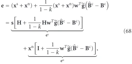
The closed-loop transfer function from the external sources (the point sources and the diffuse noise sources) to the BSS inputs (i.e, the residual signals after AFC) can be expressed in the z-domain by inserting (59) and (63) into (45):
e=(xs+xn) + 1 1−k(x
s+xn)wTgBc−Bc
=s
H+ 1 1−kHw
Tg(Bc−Bc)
es
+xn
I+ 1
1−kw
Tg(Bc−Bc)
en
,
(68)
whereBcandBcrefer to the AFC system and its ideal solution
(46), respectively, under the block-diagonal constraint (24).
k characterizes the stability of the binaural closed-loop system and is defined by (65). From (68), we can identify two independent componentsesandenpresent in the BSS inputs
and originating from the external point sources and from the diffuse noise, respectively. As mentioned in Section 4.1, the BSS algorithm allows to separate point sources, additional diffuse noise having only a limited impact on the separation performance [32]. We therefore concentrate on the first term in (68):
es=sH+s 1
1−kHw
Tg(Bc−Bc)
˘
H
, (69)
which produces an additional mixing system ˘Hintroduced by the acoustical feedback (and the required AFC filters). Ideally, the BSS filters should converge to a solution which minimizes the contribution vsint
of the interfering point sourcessintat the BSS outputv, that is,
vsint
= sintHintwT
acoustical mixing
+ sintH˘intwT
feedback loop !
=0. (70)
Hintrefers to the acoustical mixing of the interfering sources
sint, as defined inSection 2.2. ˘Hintcan be defined in a similar
way and describes the mixing of the interfering sources introduced by the feedback loop.
Acoustical paths
Acoustical mixing
Digital signal processing
A
coustic
feedback
Adaptive feedback canceler
He
a
r
in
g
-aid
pr
oc
essin
g
TDOAs
Binaural adaptive filtering
Blind source separation selectionOutput
uL uR
fLL fRL fLR fRR bL bR gL gR
vL vR
. . . . . .
. . . s1
sQ
−
− P
P
P P P P
xuL xuR
xsL
xsR
xRn xL
xR xn
L HL
HR
yL yR
eL
eR aTLL
aT RL
aTLR
aTRR
v
Figure3: Signal model of the AFC-BSS combination.
present at the BSS inputs, the BSS solution becomes biased since the algorithm will try to unravel the feedback loop ˘H instead of targetting the acoustical mixing system H only. The importance of the bias depends on the magnitude response of the filters captured by ˘Hin (70), relative to the magnitude response of the filters captured byH. Contrary to the AFC bias encountered in Section 3.2, the BSS bias therefore decreases with increasing SFR.
The above discussion concerning BSS algorithms can be generalized to any signal enhancement techniques involving adaptive filters. The presence of feedback at the algorithm’s inputs will always cause some adaptation problems. Fortu-nately, placing an AFC in front of the BAF like in Figure 1
can help increasing the SFR at the BAF inputs. In particular, when the AFC filters reach their ideal solution (i.e.,Bc=Bc),
then ˘Hbecomes zero and the bias term due to the feedback loop in (70) disappears, regardless of the amount of sound amplification applied in the forward paths.
5. Evaluation Setup
To validate the theoretical analysis conducted in Sections
3 and 4, the binaural configuration depicted in Figure 3
was experimentally evaluated for the combination of a feedback canceler and the blind source separation algorithm introduced inSection 4.1.
5.1. Algorithms. The BSS processing was performed using a two-channel version of the algorithm introduced in
Section 4.1, picking up the front microphone at each ear (i.e.,
P =1). Four adaptive BSS filters needed to be computed at each adaptation step. The output containing the target source (the most frontal one) was selected based on BSS-internal source localization (see Section 4.1, and [35]). To obtain
meaningful results which are, as far as possible, independent of the AFC implementation used, the AFC filter update was performed based on the frequency-domain adaptive filtering (FDAF) algorithm [36]. The FDAF algorithm allows for an individual step-size control for each DFT bin and a bin-wise optimum control mechanism of the step-size parameter, derived from [13,37]. In practice, this optimum step-size control mechanism is inappropriate since it requires the knowledge of signals which are not available under real conditions, but it allows us to minimize the impact of a particular AFC implementation by providing useful information on the achievable AFC performance. Since we used two microphones, the (block-diagonal constrained) AFC consisted of two adaptive filters (seeFigure 3).
Finally, to avoid other sources of interaction effects and concentrate on the AFC-BSS combination, we consid-ered a simple linear time-invariant frequency-independent hearing-aid processing in the forward paths (i.e.,gL(z)=gL
andgR(z)=gR). Furthermore, in all the results presented in
Section 4, the same HA gainsgL=gR !
=gand decorrelation delays (seeSection 3.2)DL =DR =Dwere applied at both
ears. The selected BSS output was therefore amplified by a factorg, delayed byDand played back at the two LS outputs.
5.2. Performance Measures. We saw in the previous sections that our binaural configuration significantly differs from what can usually be found in the literature on unilateral HAs. To be able to objectively evaluate the algorithms’ performance in this context, especially concerning the AFC, we need to adapt some of the already existing and commonly used performance measures to the new binaural configura-tion. This issue is discussed in the following, based on the outcomes of the theoretical analysis presented in Sections3
0
−20
−40
−60
−80
20
log
10
|
k
(
e
j
2
πf
)
|
(dB)
0 2 4 6 8
Frequencyf (kHz)
Stabilit
y
marg
in
Figure4: Illustration of the stability margin.
5.2.1. Feedback Cancellation Performance Measures. In the conventional unilateral case, the feedback cancellation per-formance is usually measured in terms of misalignment between the (single) FBP estimate and the true (single) FBP (which is the ideal solution in the unilateral case), as well as in terms of Added Stable Gain (ASG) reflecting the benefit of AFC for the user [14].
In the binaural configuration considered in this study, the misalignment should measure the mismatch between each AFC filter and its corresponding ideal solution. This can be computed in the frequency domain as follows:
bIp=10 log10
ωbIp(e
jω)−b
Ip(e jω)2
ωbIp(ejω)
2 I∈ {L, R}.
(71)
The ideal binaural AFC solution has been defined in (39) for the general case, and in (44) under the block-diagonal constraint (24) and assumption (43). In the results presented in Section 4, the misalignment has been averaged over all AFC filters (two filters in our case).
In general, it is not possible to calculate an ASG in the binaural case since the function k(ejω) characterizing the stability of the system depends on both gains gL and
gR (Section 3.3). It is however possible to calculate an
added stability margin (ASM) measuring the additional gain margin (the distance of 20log10|k(ejω)|to 0dB, seeFigure 4) obtained by the AFC
ASM=20 log10
min ω
1
k(ejω)
−20 log10
min ω
1
k(ejω)
B=0
,
(72)
wherek(z) has been defined in (57) and|k(ejω)|
B=0 is the
initial magnitude of k(z = ejω), without AFC. Since the assumption (41) is valid in our case (withcLR=1) and since
we force our AFC system to be block-diagonal, we can alter-natively use the simplified expression ofkgiven by (65). Note
that the initial stability margin 20log10(minω1/|k(ejω)|B=0)
as well as the margin with AFC 20 log10(minω1/|k(ejω)|), and hence the ASM, depend not only on the acoustical (binaural) FBPs, but also on the current state of the BAF filters. Also, whengL=gR=! g,kbecomes directly proportional togand
the ASM can be interpreted as an ASG.
Additionally, the SFR measured at the BSS and AFC inputs should be taken into account when assessing the AFC-BSS combination since it directly influences the performance of the algorithms. The SFR is defined in the following as the signal power ratio between the components coming from the external sources (without distinction between desired and interfering sources), and the components coming from loudspeakers (i.e., the feedback signals).
5.2.2. Signal Enhancement Performance Measures. The sep-aration performance of the BSS algorithm is evaluated in terms of signal-to-interference ratio (SIR), that is, the signal power ratio between the components coming from the target source and the components coming from the interfering source(s). Although the feedback components xu and the
AFC filter outputsy(i.e., the compensation signals) contain some signal coming from the external sources s (which causes a bias of the BSS solution, as discussed inSection 4), we will ignore them in the SIR calculation since these components are undesired. An SIR gain can then be obtained as the difference between the SIR at the BSS inputs and the SIR at the BSS outputs. It reflects the ability of BSS to extract the desired components from the signal mixturexs,
regardless of the amount of feedback (or background noise) present. Since only one BSS output is presented to the HA user (Section 4.1), we average the input SIR over all BSS input channels (here two), but we consider only the selected BSS output for the output SIR calculations.
5.3. Experimental Conditions. Since a two-channel ICA-based BSS algorithm can only separate two point sources (Section 4.1), no diffuse noise has been added to the sensor signal mixture (i.e.,xn=0) and only two point sources were
considered (one target source and one interfering source). Head-related impulse responses (HRIR) were measured using a pair of Siemens Life (BTE) hearing aid cases with two microphones and a single receiver (loudspeaker) inside each device (no processor). The cases were mounted on a real person and connected, via a pre-amplifier box, to a (laptop) PC equipped with a multi-channel RME Multiface sound card. Measurements were made in the following environments:
(i) a low-reverberation chamber (T60≈50 ms),
(ii) a living-room-like environment (T60≈300 ms).
The source signal components xs were then generated by
60 40 20 0 −20
(dB)
0 10 20 30 40 50
Hearing-aid gain (dB) Vent size 2 mm
Critical gain without
FBC
Reference SIRgain
SIRgain
SFRBSS in
SFRBSS out
(a)
60 40 20 0 −20
(dB)
0 10 20 30 40 50
Hearing-aid gain (dB) Vent size 3 mm
Critical gain without
FBC
Reference SIRgain
SIRgain
SFRBSS in
SFRBSS out
(b)
60 40 20 0 −20
(dB)
0 10 20 30 40 50
Hearing-aid gain (dB) Vent open
Critical gain without FBC
Reference SIRgain
SIRgain
SFRBSS in
SFRBSS out
(c)
Figure5: BSS performance for increasing HA gain, in a low-reverberation chamber.
To generate the feedback componentsxu, binaural FBPs
(“direct” and “cross” FBPs, seeSection 2.2) measured from Siemens BTE hearing aids were used. These recordings have been made for different vent sizes: 2 mm, 3 mm and open and in the following scenario:
(i) left HA mounted on a manikin without obstruction, (ii) right HA mounted on a manikin with a telephone as
obstruction.
The digital signal processing was performed at a sampling frequency of 16 kHz, picking up the front microphone at each ear (i.e.,P=1).
6. Experimental Results
In the following, experimental results involving the combi-nation of AFC and BSS are shown and discussed. BSS filters of 1024 coefficients each were applied, the AFC filter length was set to 256 and decorrelation delays of 5 ms were included in the forward paths.
6.1. Impact of Feedback on BSS. The discussion ofSection 4
indicates that a deterioration of the BSS performance is expected at low input SFR, due to a bias introduced by the feedback loop. To determine to which extent the amount of feedback deteriorates the achievable source separation, the performance of the (adaptive) BSS algorithm was experimentally evaluated for different amounts of feedback by varying the amplification levelg. Preliminary tests in the absence of AFC showed that the feedback had almost no impact on the BSS performance as long as the system was stable (i.e., as long as|k(ejω)|
B=0<1, ∀ω) because the SFR
at the BSS inputs was kept high (greater than 20 dB). This basically validates the traditional way signal enhancement techniques for hearing aids have been developed, ignoring the presence of feedback.
Signal enhancement algorithms, however, can be subject to higher input SFR levels when an AFC is used to stabilize the system. To be able to further increase the gains and the amount of feedback signal in the microphone inputs while preventing system instability, the feedback components present at the BSS outputvwere artificially suppressed. This
is equivalent to performing AFC on the BSS output, under ideal conditions. It guarantees the stability of the system (with ASM = +∞), regardless of the HA amplification level, but does not reduce the SFR at the BSS inputs. The results after convergence of the BSS algorithm are presented in Figures5 and6for different rooms and vent sizes. The reference lines show the gain in SIR achieved by BSS in the absence of feedback (and hence in the absence of AFC). The critical gain depicted by vertical dashed lines in the figures, corresponds to the maximum stable gain without AFC, that is, the gain for which the initial stability margin 20 log10(minω1/|k(ejω)|B=0) becomes zero.
At low gains, the feedback has very little impact on the SIR gain because the input SFR is sufficiently high in all tested scenarios. We see also that the interference rejection causes a decrease in SFR (from the BSS inputs to the output) since parts of the external source components are attenuated. This should be beneficial to an AFC algorithm since it reduces the bias of the AFC Wiener solution due to the interfering source, as discussed in Section 3.2. However, at high gains, where the input SFR is low (less than 10 dB), the large amount of feedback causes a significant deterioration of the interference rejection performance. Moreover, it should be noted that at low gains, the input SFR decreases proportionally to the gain, as expected. We see, however, from the figures that the input SFR suddenly drops at higher gains, when the amount of feedback becomes significant (see, e.g., the transition from
60 40 20 0 −20
(dB)
0 10 20 30 40 50
Hearing-aid gain (dB) Vent size 2 mm
Critical gain without
FBC
Reference SIRgain
SIRgain
SFRBSS in
SFRBSS out
(a)
60 40 20 0 −20
(dB)
0 10 20 30 40 50
Hearing-aid gain (dB) Vent size 3 mm
Critical gain without
FBC
Reference SIRgain
SIRgain
SFRBSS in
SFRBSS out
(b)
60 40 20 0 −20
(dB)
0 10 20 30 40 50
Hearing-aid gain (dB) Vent open
Critical gain without FBC
Reference SIRgain
SIRgain
SFRBSS in
SFRBSS out
(c)
Figure6: BSS performance for increasing HA gain, in a living-room environment.
60 40 20 0 −20 −40
(dB)
0 10 20 30 40 50
Hearing-aid gain (dB) Low-reverberation chamber
Reference SIRgain
SIRgain
SFRBSS in
SFRFBC in
ASM Misalignment (a)
60 40 20 0 −20 −40
(dB)
0 10 20 30 40 50
Hearing-aid gain (dB) Living room environment
Reference SIRgain
SIRgain
SFRBSS in
SFRFBC in
ASM Misalignment (b)
Figure7: Performance of the AFC-BSS combination in two acoustical environments. The measured FPBs for a vent of size 2 mm were used.
more important since it acts mainly in favor of the target source. This second mechanism illustrates the impact of the feedback loop on the BSS algorithm at high feedback levels. It shows the necessity to have the AFC placed before BSS, so that BSS can benefit from a higher input SFR.
6.2. Overall Behavior of the AFC-BSS Combination. The full AFC-BSS combination has been evaluated for a vent size of 2 mm, in the low-reverberation chamber as well as in the living-room-like environment (Section 5.3).Figure 7depicts the BSS and AFC performance obtained after convergence. Like in Figures5and6, the reference lines show the gain in SIR achieved by BSS in the absence of feedback (and hence in the absence of AFC).
The results confirm the observations made in the pre-vious section. With the AFC applied directly on the sensor signals, the BSS algorithm could indeed benefit from the ability of the AFC to keep the SFR at the BSS inputs at high levels for every considered HA gains. Therefore, BSS always provided SIR gains which were very close to the reference SIR gain obtained without feedback, even at high gains. This contrasts with the results obtained in Figures5and6, where an ideal AFC was applied at the BSS output instead of being applied first.
Note that the SFR at the AFC outputs correspond here to the SFR at the BSS inputs. The gain in SFR (SFRBSSin − SFRAFCin, i.e., the feedback attenuation) achieved by the AFC
This is confirmed here by the SIR results shown in the figures. The difference in AFC performance comes therefore from the higher amount of residual interfering signal present at the LS outputs in the living-room-like environment, which increases the bias of the AFC Wiener solution.
The AFC does not suffer from any particular negative interactions with the BSS algorithm since it comes first in the processing chain, but rather benefits from BSS, especially in the low-reverberation chamber, as we just saw. Note that the situation is very different when the AFC is applied after BSS. In this case, the AFC filters need to quickly follow the continuously time-varying BSS filters, which prevents proper convergence of the AFC filters, even with time-invariant FBPs.
7. Conclusions
An analysis of a system combining adaptive feedback cancel-lation and adaptive binaural filtering for signal enhancement in hearing aids was presented. To illustrate our study, a blind source separation algorithm was chosen as an example for adaptive binaural filtering. A number of interaction effects could be identified. Moreover, to correctly understand the behavior of the AFC, the system was described and analyzed in detail. A new stability condition adapted to the binaural configuration could be derived, and adequate performance measures were proposed which account for the specificities of the binaural system. Experimental evaluations confirmed and illustrated the theoretical findings.
The ideal AFC solution in the new binaural configuration could be identified but a steady-state analysis showed that the AFC suffers from a bias in its optimum (Wiener) solution. This bias, similar to the unilateral case, is due to the correlation between feedback and external source signals. It was also demonstrated theoretically as well as experimentally that a signal enhancement algorithm could help reducing this bias. The correlation between feedback and external source signals also causes a bias of the BAF solution. But contrary to the bias encountered by the AFC, the BAF bias increases with increasing HA amplification levels. Fortunately, this bias can be reduced by applying AFC on the sensor signals directly, instead of applying it on the BAF outputs.
The analysis also showed that two SIMO AFC systems of adaptive filters can effectively compensate for the four SIMO FBP systems when the outputs are sufficiently correlated (see
Section 3.1). Should this condition not be fulfilled because of, for example, some non-linearities in the forward paths, the “cross” feedback signals travelling from one ear to the other would not be completely identifiable. But we saw that since the amplitude of the “cross” FBPs is usually negligible compared to the amplitude of the “direct” FBPs, the consequences would be very limited as long as the HA gains are set to similar amplification levels.
Acknowledgments
This work has been supported by a grant from the Europ-ean Union FP6 Project 004171 HEARCOM (
http://hear-com.eu/main de.html). We would also like to thank Siemens Audiologische Technik, Erlangen, for providing some of the hearing-aid recordings for evaluation.
References
[1] S. Doclo and M. Moonen, “GSVD-based optimal filtering for single and multimicrophone speech enhancement,”IEEE Transactions on Signal Processing, vol. 50, no. 9, pp. 2230–2244, 2002.
[2] A. Spriet, M. Moonen, and J. Wouters, “Spatially pre-processed speech distortion weighted multi-channel Wiener filtering for noise reduction,”Signal Processing, vol. 84, no. 12, pp. 2367–2387, 2004.
[3] S. Doclo, A. Spriet, M. Moonen, and J. Wouters, “Design of a robust multi-microphone noise reduction algorithm for hearing instruments,” inProceedings of the International Symposium on Mathematical Theory of Networks and Systems (MTNS ’04), pp. 1–9, Leuven, Belgium, July 2004.
[4] J. Vanden Berghe and J. Wouters, “An adaptive noise canceller for hearing aids using two nearby microphones,”Journal of the Acoustical Society of America, vol. 103, no. 6, pp. 3621–3626, 1998.
[5] D. P. Welker, J. E. Greenberg, J. G. Desloge, and P. M. Zurek, “Microphone-array hearing aids with binaural output—part II: a two-microphone adaptive system,”IEEE Transactions on Speech and Audio Processing, vol. 5, no. 6, pp. 543–551, 1997. [6] M. Doerbecker and S. Ernst, “Combination of two-channel
spectral subtraction and adaptive Wiener post-filtering for noise reduction and dereverberation,” in Proceedings of the 8th European Signal Processing Conference (EUSIPCO ’96), pp. 995–998, Trieste, Italy, September 1996.
[7] T. J. Klasen, T. van den Bogaert, M. Moonen, and J. Wouters, “Binaural noise reduction algorithms for hearing aids that preserve interaural time delay cues,” IEEE Transactions on Signal Processing, vol. 55, no. 4, pp. 1579–1585, 2007. [8] S. Doclo, R. Dong, T. J. Klasen, J. Wouters, S. Haykin, and
M. Moonen, “Extension of the multi-channel Wiener filter with ITD cues for noise reduction in binaural hearing aids,” in Proceedings of IEEE Workshop on Applications of Signal Processing to Audio and Acoustics (WASPAA ’05), pp. 70–73, New Paltz, NY, USA, October 2005.
[9] T. J. Klasen, S. Doclo, T. van den Bogaert, M. Moonen, and J. Wouters, “Binaural multi-channel Wiener filtering for hearing aids: preserving interaural time and level differences,” inProceedings of IEEE International Conference on Acoustics, Speech and Signal Processing (ICASSP ’06), vol. 5, pp. 145–148, Toulouse, France, May 2006.
[10] R. Aichner, H. Buchner, M. Zourub, and W. Kellermann, “Multi-channel source separation preserving spatial infor-mation,” inProceedings of IEEE International Conference on Acoustics, Speech, and Signal Processing (ICASSP ’07), vol. 1, pp. 5–8, Honolulu, Hawaii, USA, May 2007.
[11] D. P. Egolf, “Review of the acoustic feedback literature for a control systems point of view,” inThe Vanderbilt Hearing-Aid Report, pp. 94–103, York Press, London, UK, 1982.
[12] M. G. Siqueira and A. Alwan, “Steady-state analysis of continuous adaptation in acoustic feedback reduction systems for hearing-aids,” IEEE Transactions on Speech and Audio Processing, vol. 8, no. 4, pp. 443–453, 2000.