Volume 2006, Article ID 20858, Pages1–23 DOI 10.1155/ASP/2006/20858
A Constrained Least Squares Approach to Mobile Positioning:
Algorithms and Optimality
K. W. Cheung,1H. C. So,1W.-K. Ma,2and Y. T. Chan3
1Department of Electronic Engineering, City University of Hong Kong, Tat Chee Avenue, Kowloon, Hong Kong 2Department of Electrical Engineering, National Tsing Hua University, Hsinchu 30013, Taiwan
3Department of Electrical & Computer Engineering, Royal Military College of Canada, Kingston, ON, Canada K7K 7B4
Received 20 May 2005; Revised 25 November 2005; Accepted 8 December 2005
The problem of locating a mobile terminal has received significant attention in the field of wireless communications. Time-of-arrival (TOA), received signal strength (RSS), time-difference-of-arrival (TDOA), and angle-of-arrival (AOA) are commonly used measurements for estimating the position of the mobile station. In this paper, we present a constrained weighted least squares (CWLS) mobile positioning approach that encompasses all the above described measurement cases. The advantages of CWLS in-clude performance optimality and capability of extension to hybrid measurement cases (e.g., mobile positioning using TDOA and AOA measurements jointly). Assuming zero-mean uncorrelated measurement errors, we show by mean and variance analysis that all the developed CWLS location estimators achieve zero bias and the Cram´er-Rao lower bound approximately when measurement error variances are small. The asymptotic optimum performance is also confirmed by simulation results.
Copyright © 2006 Hindawi Publishing Corporation. All rights reserved.
1. INTRODUCTION
Accurate positioning of a mobile station (MS) will be one of the essential features that assists third generation (3G) wireless systems in gaining a wide acceptance and trigger-ing a large number of innovative applications. Although the main driver of location services is the requirement of lo-cating Emergency 911 (E-911) callers within a specified ac-curacy in the United States [1], mobile position informa-tion will also be useful in monitoring of the mentally im-paired (e.g., the elderly with Alzheimer’s disease), young children and parolees, intelligent transport systems, location billing, interactive map consultation and location-dependent e-commerce [2–6]. Global positioning system (GPS) could be used to provide mobile location, however, it would be expensive to be adopted in the mobile phone network be-cause additional hardware is required in the MS. Alterna-tively, utilizing the base stations (BSs) in the existing net-work for mobile location is preferable and is more cost eff ec-tive for the consumer. The basic principle of this software-based solution is to use two or more BSs to intercept the MS signal, and common approaches [6–8] are based on time-of-arrival (TOA), received signal strength (RSS), time-difference-of-arrival (TDOA), and/or angle-of-arrival (AOA) measurements determined from the MS signal re-ceived at the BSs.
In the TOA method, the distance between the MS and BS is determined from the measured one-way propagation time of the signal traveling between them. For two-dimensional (2D) positioning, this provides a circle centered at the BS on which the MS must lie. By using at least three BSs to re-solve ambiguities arising from multiple crossings of the lines of position, the MS location estimate is determined by the intersection of circles. The RSS approach employs the same trilateration concept where the propagation path losses from the MS to the BSs are measured to give their distances. In the TDOA method, the differences in arrival times of the MS sig-nal at multiple pairs of BSs are measured. Each TDOA mea-surement defines a hyperbolic locus on which the MS must lie and the position estimate is given by the intersection of two or more hyperbolas. Finally, the AOA method necessi-tates the BSs to have multielement antenna arrays for mea-suring the arrival angles of the transmitted signal from the MS at the BSs. From each AOA estimate, a line of bearing (LOB) from the BS to the MS can be drawn and the position of the MS is calculated from the intersection of a minimum of two LOBs. In general, the MS position is not determined geometrically but is estimated from a set of nonlinear equa-tions constructed from the TOA, RSS, TDOA, or AOA mea-surements, with knowledge of the BS geometry.
directly in a nonlinear least squares (NLS) or weighted least squares (WLS) framework. Although optimum estimation performance can be attained, it requires sufficiently precise initial estimates for global convergence because the corre-sponding cost functions are multimodal. The second ap-proach [13–17] is to reorganize the nonlinear equations into a set of linear equations so that real-time implementation is allowed and global convergence is ensured. In this paper, the latter approach is adopted, and we will focus on a unified de-velopment of accurate location algorithms, given the TOA, RSS, TDOA, and/or AOA measurements.
For TDOA-based location systems, it is well known that for sufficiently small noise conditions, the corresponding nonlinear equations can be reorganized into a set of linear equations by introducing an intermediate variable, which is a function of the source position, and this technique is com-monly called spherical interpolation (SI) [13]. However, the SI estimator solves the linear equations via standard least squares (LS) without using the known relation between the intermediate variable and the position coordinate. To im-prove the location accuracy of the SI approach, Chan and Ho have proposed [14] to use a two-stage WLS to solve for the source position by exploiting this relation implic-itly via a relaxation procedure, while [15] incorporates the relation explicitly by minimizing a constrained LS function based on the technique of Lagrange multipliers. According to [15], these two modified algorithms are referred to as the quadratic correction least squares (QCLS) and linear correc-tion least squares (LCLS), respectively. Recently, we have im-proved [18] the performance of the LCLS estimator by in-troducing a weighting matrix in the optimization, which can be regarded as a hybrid version of the QCLS and LCLS algo-rithms. The idea of this constrained weighted least squares (CWLS) technique has also been extended to the RSS [19] and TOA [20] measurements. Using a different way of con-verting nonlinear equations to linear equations without in-troducing dummy variables, Pages-Zamora et al. [16] have developed a simple LS AOA-based location algorithm. In this work, our contributions include (i) development of a unified approach for mobile location which allows utilizing different combinations of TOA, RSS, TDOA, and AOA measurements via generalizing [18–20] and improving [16] with the use of WLS; and (ii) derivation of bias and variance expressions for all the proposed algorithms. In particular, we prove that the performance of all the proposed estimation methods can achieve zero bias and the Cram´er-Rao lower bound (CRLB) [21] approximately when the measurement errors are uncor-related and small in magnitude.
The rest of this paper is organized as follows. InSection 2, we formulate the models for the TOA, TDOA, RSS, and AOA measurements and state our assumptions. InSection 3, three CWLS location algorithms using TDOA, RSS, and TOA measurements, respectively, are first reviewed, and a WLS AOA-based location algorithm is then devised via modi-fying [16]. Mobile location using various combinations of TOA, TDOA, RSS, and AOA measurements is also examined. In particular, a TDOA-AOA hybrid algorithm is presented in detail. The performance of all the developed algorithms
Table1: List of abbreviations and symbols. AOA Angle-of-arrival
CWLS Constrained weighted least squares CRLB Cram´er-Rao lower bound NLS Nonlinear least squares RSS Received signal strength TOA Time-of-arrival
TDOA Time-difference-of-arrival AT Transpose of matrixA A−1 Inverse of matrixA
Ao Optimum matrix ofA
σ2 Noise variance
Cn Noise covariance matrix
I(x) Fisher information matrix for parameter vectorx
x Optimization variable vector forx
x Estimate ofx
diag(x) Diagonal matrix formed from vectorx IM M×Midentity matrix
1M M×1 column vector with all ones 0M M×1 column vector with all zeros OM×N M×Nmatrix with all zeros
Element-by-element multiplication
is studied in Section 4. Simulation results are presented in
Section 5to evaluate the location estimation performance of the proposed estimators and verify our theoretical findings. Finally, conclusions are drawn inSection 6. A list of abbre-viations and symbols that are used in the paper is given in
Table 1.
2. MEASUREMENT MODELS
In this section, the models and assumptions for the TOA, TDOA, RSS, and AOA measurements are described. Letx= [x,y]T be the MS position to be determined and let the
known coordinates of theith BS bexi = [xi,yi]T,i = 1, 2,
. . .,M, where the superscriptTdenotes the transpose opera-tion andMis the total number of receiving BSs. The distance between the MS and theith BS, denoted bydi, is given by
di=x−xi 2
+y−yi 2
,i=1, 2,. . .,M. (1)
2.1. TOA measurement
The TOA is the one-way propagation time taken for the sig-nal to travel from the MS to a BS. In the absence of distur-bance, the TOA measured at theith BS, denoted byti, is
ti=di
wherecis the speed of light. The range measurement based on ti in the presence of disturbance, denoted by rTOA,i, is
modeled as
rTOA,i=di+nTOA,i
=x−xi 2
+y−yi 2
+nTOA,i, i=1, 2,. . .,M,
(3)
wherenTOA,iis the range error inrTOA,i. Equation (3) can also
be expressed in vector form as
rTOA=fTOA(x) +nTOA, (4)
where
rTOA=
rTOA,1rTOA,2· · ·rTOA,M T
,
nTOA=
nTOA,1nTOA,2· · ·nTOA,M T
,
fTOA(x)=
⎡ ⎢ ⎢ ⎢ ⎢ ⎢ ⎢ ⎢ ⎢ ⎣
x−x12+y−y12
x−x22+y−y22 ..
.
x−xM 2
+y−yM 2
⎤ ⎥ ⎥ ⎥ ⎥ ⎥ ⎥ ⎥ ⎥ ⎦
.
(5)
2.2. TDOA measurement
The TDOA is the difference in TOAs of the MS signal at a pair of BSs. Assigning the first BS as the reference, it can be easily deduced that the range measurements based on the TDOAs are of the form
rTDOA,i=
di−d1
+nTDOA,i
=x−xi 2
+y−yi 2
−x−x12+y−y12
+nTDOA,i, i=2, 3,. . .,M,
(6)
wherenTDOA,iis the range error inrTDOA,i. Notice that if the
TDOA measurements are directly obtained from the TOA data, thennTDOA,i=nTOA,i−nTOA,1,i=2, 3,. . .,M. In vector
form, (6) becomes
rTDOA=fTDOA(x) +nTDOA, (7)
where
rTDOA=
rTDOA,2rTDOA,3· · ·rTDOA,M T
,
nTDOA=
nTDOA,2nTDOA,3· · ·nTDOA,M T
,
fTDOA(x)=
⎡ ⎢ ⎢ ⎢ ⎢ ⎢ ⎢ ⎢ ⎢ ⎢ ⎣
x−x22+y−y22−x−x12+y−y12
x−x32+y−y32−x−x12+y−y12 ..
.
x−xM 2
+y−yM 2
−x−x12+y−y12
⎤ ⎥ ⎥ ⎥ ⎥ ⎥ ⎥ ⎥ ⎥ ⎥ ⎦
.
(8)
2.3. RSS measurement
Without measurement error, the RSS or received power at theith BS, denoted byPir, can be modeled as [22]
Pr i =KiP
t i
dai
, i=1, 2,. . .,M, (9)
wherePti is the transmitted power,Kiaccounts for all other
factors which affect the received power, including the an-tenna height and anan-tenna gain, andais the propagation con-stant. Note that the propagation parameteracan be obtained via finding the path loss slope by measurement [22]. In free space,ais equal to 2, but in some urban and suburban areas, acan vary from 3 to 6. From (9), the range measurements based on the RSS data with the use of the known{Pt
i}and
{Ki}, denoted by{rRSS,i}, are determined as
rRSS,i=KiP t i
Pr i
+nRSS,i
=x−xi 2
+y−yi 2a/2
+nRSS,i, i=1, 2,. . .,M,
(10)
wherenRSS,iis the range error inrRSS,i. It is noteworthy that
ifa=1, then (10) will be of the same form as (3). Equation (10) can also be expressed in vector form as
rRSS=fRSS(x) +nRSS, (11)
where
rRSS=
rRSS,1rRSS,2· · ·rRSS,M T
,
nRSS=
nRSS,1nRSS,2· · ·nRSS,M T
,
fRSS(x)=
⎡ ⎢ ⎢ ⎢ ⎢ ⎢ ⎢ ⎢ ⎢ ⎢ ⎢ ⎢ ⎣
x−x12+y−y12a/2
x−x22+y−y22a/2 ..
.
x−xM 2
+y−yM 2a/2
⎤ ⎥ ⎥ ⎥ ⎥ ⎥ ⎥ ⎥ ⎥ ⎥ ⎥ ⎥ ⎦
.
2.4. AOA measurement
The AOA of the transmitted signal from the MS at theith BS, denoted byφi, is related toxandxiby
tanφi
= y−yi
x−xi
, i=1, 2,. . .,M. (13)
Geometrically,φiis the angle between the LOB from theith
BS to the MS and thex-axis. The AOA measurements in the presence of angle errors, denoted by{rAOA,i}, are modeled as
rAOA,i=φi+nAOA,i=tan−1 y−y
i
x−xi
+nAOA,i, i=1, 2,. . .,M,
(14)
wherenAOA,iis the noise inrAOA,i. Equation (14) can also be
expressed in vector form as
rAOA=fAOA(x) +nAOA, (15)
where
rAOA=
rAOA,1rAOA,2· · ·rAOA,M T
,
nAOA=
nAOA,1nAOA,2· · ·nAOA,M T
,
fAOA(x)=
⎡ ⎢ ⎢ ⎢ ⎢ ⎢ ⎢ ⎢ ⎢ ⎢ ⎢ ⎢ ⎢ ⎣
tan−1
y−y1 x−x1
tan−1
y−y2 x−x2
.. .
tan−1
y−yM
x−xM
⎤ ⎥ ⎥ ⎥ ⎥ ⎥ ⎥ ⎥ ⎥ ⎥ ⎥ ⎥ ⎥ ⎦
.
(16)
To facilitate the development and analysis of the pro-posed location algorithms, we make the following assump-tions for the TOA, TDOA, RSS, and AOA measurements.
(A1) All measurement errors, namely,{nTOA,i},{nTDOA,i},
{nRSS,i}, and {nAOA,i} are sufficiently small and are
modeled as zero-mean Gaussian random variables with known covariance matrices, denoted by Cn,TOA,
Cn,TDOA, Cn,RSS, and Cn,AOA, respectively. The zero-mean error assumption implies that multipath and non-line-of-sight (NLOS) errors have been mitigated, which can be done by considering the techniques in [23–27]. Nevertheless, the effect of NLOS propaga-tion will be studied inSection 5for the TOA measure-ments.
(A2) For RSS-based location, the propagation parametera is known and has a constant value for all RSS measure-ments.
(A3) The numbers of BSs for location using the TOA, TDOA, RSS, and AOA measurements are at least 3, 4, 3, and 2, respectively.
3. ALGORITHM DEVELOPMENT
This section describes our development of the CWLS/WLS mobile positioning approach for the cases of TDOA, RSS, TOA, and AOA measurements. We also discuss how the proposed methods can be extended to hybrid measurement cases, such as the TDOA-AOA.
3.1. TDOA [18]
Without disturbance, (6) becomes
rTDOA,i=
x−xi 2
+y−yi 2
−x−x12+y−y12
=⇒rTDOA,i+
x−x12+y−y12
=x−xi 2
+y−yi 2
, i=2, 3,. . .,M.
(17)
Squaring both sides of (17) and introducing an intermediate variable,R1, which has the form
R1=d1=x−x12+y−y12, (18)
we obtain the following set of linear equations [13]
x−x1xi−x1
+y−y1yi−y1
+rTDOA,iR1
=1 2
xi−x1 2
+yi−y1 2
−r2 TDOA,i
, i=2, 3,. . .,M.
(19)
Writing (19) in matrix form gives
Gϑ=h, (20)
where
G=
⎡ ⎢ ⎢ ⎢ ⎢ ⎣
x2−x1 y2−y1 rTDOA,2 ..
. ... ...
xM−x1 yM−y1 rTDOA,M ⎤ ⎥ ⎥ ⎥ ⎥ ⎦,
h=1
2
⎡ ⎢ ⎢ ⎢ ⎢ ⎢ ⎣
x2−x12+y2−y12−r2TDOA,2 ..
.
xM−x1 2
+yM−y1 2
−r2 TDOA,M
⎤ ⎥ ⎥ ⎥ ⎥ ⎥ ⎦,
(21)
and the parameter vectorϑ=[x−x1,y−y1,R1]Tconsists of
In the presence of measurement errors, the SI technique determines the MS position by simply solving (20) via stan-dard LS, and the location estimate is found from [13]
ϑ=arg min ˘ ϑ (G
˘
ϑ−h)T(Gϑ˘−h)
=GTG−1GTh,
(22)
where ˘ϑ=[ ˘x−x1, ˘y−y1, ˘R1]T is an optimization variable
vector and−1represents the matrix inverse, without utilizing the known relationship between ˘x, ˘y, and ˘R1.
An improvement to the SI estimator is the LCLS method [15], which solves the LS cost function in (22) subject to the constraint of ( ˘x−x1)2+ ( ˘y−y1)2=R˘2
1, or equivalently,
˘
ϑTΣϑ˘=0, (23)
whereΣ=diag(1, 1,−1).
On the other hand, Chan and Ho [14] have improved the SI estimator through two stages. In the first stage of the QCLS estimator, a coarse estimate is computed by minimiz-ing a WLS function
(Gϑ˘−h)TΥ−1(Gϑ˘−h), (24)
whereΥis a symmetric weighting matrix, which is a function of the estimate ofR1, denoted byR1 . A better estimate ofϑis then obtained in the second stage via minimizing ( ˘x−x1)2+ ( ˘y−y1)2−R˘2
1 according to another WLS procedure. Since
R1is not available at the beginning, normally a few iterations between the two stages are required to attain the best solution [15].
The idea of our CWLS estimator is to combine the key principles in the CWLS and LCLS methods, that is, the MS position estimate is determined by minimizing (24) subject to (23). For sufficiently small measurement errors, the in-verse of the optimum weighting matrixΥ−1 for the CWLS algorithm is found using the best linear unbiased estimator (BLUE) [21] as in [14]:
Υo=s
1sT1 Cn,TDOA, (25)
where
s1=
⎡ ⎢ ⎢ ⎢ ⎢ ⎢ ⎢ ⎢ ⎣
d2 d3 .. .
dM ⎤ ⎥ ⎥ ⎥ ⎥ ⎥ ⎥ ⎥ ⎦
=
⎡ ⎢ ⎢ ⎢ ⎢ ⎢ ⎢ ⎣
d2−d1+R1 d3−d1+R1
.. .
dM−d1+R1 ⎤ ⎥ ⎥ ⎥ ⎥ ⎥ ⎥ ⎦
(26)
anddenotes element-by-element multiplication. SinceΥ contains the unknown{di}, we expressdi = di−d1+R1
and approximatedi−d1byrTDOA,iand thus an approximate
version ofΥo, namely,s
1sT1 Cn,TDOAwiths1 = [rTDOA,2+
R1· · ·rTDOA,M+R1 ]Tis employed in practice.
Similar to [15], the CWLS problem is solved by using the technique of Lagrange multipliers and the Lagrangian to be minimized is
LTDOA(˘ϑ,η)=(Gϑ˘−h)TΥ−1(Gϑ˘−h) +ηϑ˘
T
Σϑ˘, (27)
whereηis the Lagrange multiplier to be determined. The es-timate of ϑis obtained by differentiatingLTDOA(˘ϑ,η) with respect to ˘ϑand then equating the results to zero (see Appen-dix A.1):
ϑ=GTΥ−1G+ηΣ−1GTΥ−1h, (28)
whereηis found from the following 4-root equation:
3
i=1 αiβi
η+ζi
2 =0 (29)
and{αi},{βi}, and{ζi},i=1, 2, 3, have been defined in Ap-pendix A.1. The procedure for CWLS TDOA-based location is summarized as follows.
(i) SetΥ=IM−1, whereIM−1denotes the identity matrix of dimension (M−1).
(ii) Find all roots of (29) by using a standard root finding algorithm. Then take only the real roots into consider-ation as the Lagrange multiplier is always real for a real optimization problem.
(iii) Put the realη’s back to (28) and obtain subestimates of
ϑ. Then choose the solutionϑfrom those subestimates which makes the expression (Gϑ˘ −h)TΥ−1(Gϑ˘−h) minimum.
(iv) ConstructΥaccording to (25) using the obtainedR1 in step (iii). Then, repeat steps (ii) and (iii) untilϑ con-verges.
3.2. RSS [19]
Without measurement errors, (10) becomes
rRSS,i=
x−xi 2
+y−yi 2a/2
, i=1, 2,. . .,M. (30)
Extending the SI technique and taking power 2/aon both sides of (30) yields
rRSS,2/ai=R22−2xxi−2y yi+
x2i +y2i
=⇒xix+yiy−0.5R22
=1 2
x2
i +yi2−ri2/a
, i=1, 2,. . .,M,
(31)
where
is the introduced intermediate variable in order to linearize (30) in terms ofx,y, andR2
2. Similar to the TDOA measure-ments, (31) can be expressed in matrix-vector form:
Aθ=b, (33)
where
A=
⎡ ⎢ ⎢ ⎢ ⎢ ⎣
x1 y1 −0.5 ..
. ... ...
xM yM −0.5 ⎤ ⎥ ⎥ ⎥ ⎥
⎦, θ=
⎡ ⎢ ⎢ ⎢ ⎣
x
y
R2 2
⎤ ⎥ ⎥ ⎥ ⎦,
b=1
2
⎡ ⎢ ⎢ ⎢ ⎢ ⎣
x2
1+y21−rRSS,12/a .. .
x2
M+yM2 −rRSS,2/aM ⎤ ⎥ ⎥ ⎥ ⎥ ⎦.
(34)
The CWLS estimate ofθis obtained by minimizing
(Aθ˘−b)TΨ−1(Aθ˘−b), (35)
whereΨ−1is the corresponding weighting matrix, subject to
qTθ˘+ ˘θTPθ˘=0 (36)
such that
˘
θ=
⎡ ⎢ ⎢ ⎢ ⎣
˘ x ˘ y ˘ R2
⎤ ⎥ ⎥ ⎥
⎦, P=
⎡ ⎢ ⎢ ⎢ ⎣
1 0 0
0 1 0
0 0 0
⎤ ⎥ ⎥ ⎥
⎦, q=
⎡ ⎢ ⎢ ⎢ ⎣
0
0 −1
⎤ ⎥ ⎥ ⎥
⎦. (37)
Here, (36) is a matrix characterization of the relation in (32). The optimum value ofΨis also determined based on the BLUE as follows. For sufficiently small measurement errors, the value ofrRSS,2/aican be approximated as
rRSS,2/ai=
dai +nRSS,i 2/a
≈d2
i +
2 a
di 2−a
nRSS,i, i=1, 2,. . .,M.
(38)
As a result, the disturbance between the true and estimate of the squared distances is
εi=rRSS,2/ai−d2i ≈
2 a
di 2−a
nRSS,i, i=1, 2,. . .,M. (39)
In vector form,{εi}is expressed as
ε=
2 a
d12−anRSS,1,2 a
d22−anRSS,2,. . .,2 a
dM 2−a
nRSS,M T
.
(40)
The covariance matrix of the disturbance, which leads to the optimum weighting matrix, is thus of the form
Ψo=EεεT=s
2sT2 Cn,RSS, (41)
where
s2=
1 a
d12−a 1 a
d22−a · · · 1 a
dM 2−aT
. (42)
Sinces2depends on the unknowns{di}, we use{ri1/a}instead
of{di}to form an estimate ofs2, denoted bys2, which is
s2=
1 ar
2/a−1 RSS,1
1 ar
2/a−1 RSS,2 · · ·
1 ar
2/a−1 RSS,M
T
. (43)
Minimizing (35) subject to (36) is equivalent to minimizing the Lagrangian
LRSS( ˘θ,λ)=(Aθ˘−b)TΨ−1(Aθ˘−b) +λ
qTθ˘+ ˘θT
Pθ˘, (44)
whereλis the corresponding Lagrange multiplier. The CWLS solution using the RSS measurements is given by (see Appen-dix A.2)
θ=ATΨ−1A+λP−1ATΨ−1b−λ
2q
, (45)
whereλis determined from the 5-root equation:
c3f3−λ 2c3g3+
2
i=1 cifi
1 +λγi−
λ 2
2
i=1 cigi
1 +λγi+
2
i=1 eifiγi
1 +λγi 2
−λ 2
2
i=1 eigiγi
1+λγi 2−
λ 2
2
i=1 cifiγi
1+λγi 2+
λ2 4
2
i=1 cigiγi
1+λγi 2 =0.
(46)
The{ci},{ei},{fi}, and{gi},i=1, 2, 3, have been defined in Appendix A.2. The CWLS solution using the RSS measure-ments is found by the following procedure.
(i) Obtain the real roots of (46) using a root finding algo-rithm.
(ii) Put the realλ’s back to (45) and obtain subestimates of
θ.
3.3. TOA [20]
Since the models of the TOA and RSS will have the same form if the propagation constant is equal to unity, puttinga=1 in
Section 3.2yields the algorithm of the CWLS estimator using the TOA data.
3.4. AOA
In the absence of noise, (13) becomes
tanrAOA,i
= sin
rAOA,i
cosrAOA,i
= y−yi
x−xi, i=1, 2,. . .,M.
(47)
By cross-multiplying and rearranging (47), a set of linear equations inxandyfor the AOA measurements is obtained as
xsinrAOA,i
−ycosrAOA,i
=xisin
rAOA,i
−yicos
rAOA,i
, i=1, 2,. . .,M. (48)
Expressing (48) in matrix form, we have [16]
Hx=k, (49)
where
H=
⎡ ⎢ ⎢ ⎢ ⎢ ⎣
sinrAOA,1 −cosrAOA,1 ..
. ...
sinrAOA,M
−cosrAOA,M
⎤ ⎥ ⎥ ⎥ ⎥ ⎦,
k=
⎡ ⎢ ⎢ ⎢ ⎢ ⎣
x1sinrAOA,1−y1cosrAOA,1 ..
.
xMsin
rAOA,M
−yMcos
rAOA,M
⎤ ⎥ ⎥ ⎥ ⎥ ⎦.
(50)
To improve the performance of the LS estimator of [16], we propose to use WLS to estimate the MS locationxand the solution is
x=arg min ˘
x (Hx˘−k)
TΩ−1(Hx˘−k)
=HTΩ−1H−1HTΩ−1k,
(51)
whereΩ−1is the corresponding weighting matrix and ˘x = [ ˘x, ˘y]T. Again, we use the BLUE technique to determine the
optimumΩas follows. In the presence of measurement er-rors, (48) becomes
xsinφi+nAOA,i
−ycosφi+nAOA,i
=xisin
φi+nAOA,i
−yicos
φi+nAOA,i
, i=1, 2,. . .,M. (52)
It is noteworthy that (52) is similar to the Taylor series lin-earization based on a geometrical viewpoint [17], although the latter considers only one AOA measurement with the cor-responding BS locates at the origin. By expanding sin(φi+
nAOA,i) and cos(φi+nAOA,i), and considering sufficiently small
angle errors such that sin(nAOA,i)≈nAOA,iand cos(nAOA,i)≈
1, we obtain the residual error inrAOA,ias
δi=nAOA,i
x−xi
cosφi
+y−yi
sinφi
,
i=1, 2,. . .,M. (53)
In vector form,{δi}is expressed as
δ=
⎡ ⎢ ⎢ ⎢ ⎢ ⎢ ⎢ ⎢ ⎣
nAOA,1x−x1cosφ1+y−y1sinφ1 nAOA,2x−x2cosφ2+y−y2sinφ2
.. .
nAOA,M
x−xM
cosφM
+y−yM
sinφM
⎤ ⎥ ⎥ ⎥ ⎥ ⎥ ⎥ ⎥ ⎦
.
(54)
Thus the inverse of the optimum weighting matrix,Ωo, is
Ωo=EδδT=
s3sT3 Cn,AOA, (55)
where
s3=
⎡ ⎢ ⎢ ⎢ ⎢ ⎢ ⎢ ⎣
x−x1cosφ1+y−y1sinφ1
x−x2cosφ2+y−y2sinφ2 ..
.
x−xM
cosφM
+y−yM
sinφM
⎤ ⎥ ⎥ ⎥ ⎥ ⎥ ⎥ ⎦
=
⎡ ⎢ ⎢ ⎢ ⎢ ⎢ ⎢ ⎢ ⎣
d1 d2 .. .
dM ⎤ ⎥ ⎥ ⎥ ⎥ ⎥ ⎥ ⎥ ⎦
(56)
because cos(φi)=(x−xi)/diand sin(φi)=(y−yi)/di. Again,
sinces3involves the unknown parametersxand{φi}, they
will be approximated asx and{rAOA,i}, respectively, in the
actual implementation. In summary, the WLS procedure for AOA-based location is
(i) setΩ=IM;
(ii) use (51) to determine the estimate ofx;
(iii) constructΩbased on (55) using the computed xin step (ii) and repeat step (ii) until parameter conver-gence.
It is noteworthy that sinceHalso consists of noise, we have already attempted to introduce constraints in the WLS solution in order to remove the bias due to the noisy com-ponents, but improvement over the WLS estimator has not been observed. As a result, it is believed that the noise in
3.5. TDOA-AOA hybrid
It is apparent that combining different types of the mea-surements, if available, can improve location performance and/or reduce the number of receiving BSs. Among various hybrid schemes, the most popular one is to use the TDOA and AOA measurements simultaneously [17]. To perform TDOA-AOA mobile positioning, (48) is now rewritten by addingy1cos(rAOA,i)−x1sin(rAOA,i) on both sides:
x−x1sinrAOA,i
−y−y1cosrAOA,i
=xi−x1
sinrAOA,i
−yi−y1
cosrAOA,i
,
i=1, 2,. . .,M. (57)
Combining (19) and (57) into a single matrix-vector form yields
Bϑ=w, (58)
where
B=
⎡
⎣ G
H 0M
⎤
⎦, w=
⎡ ⎣h
k ⎤ ⎦,
k=
⎡ ⎢ ⎢ ⎢ ⎢ ⎢ ⎢ ⎢ ⎣
0
x2−x1sinrAOA,2−y2−y1cosrAOA,2 ..
.
xM−x1
sinrAOA,M
−yM−y1
cosrAOA,M
⎤ ⎥ ⎥ ⎥ ⎥ ⎥ ⎥ ⎥ ⎦
(59)
with0M is anM×1 column vector with all zeros. Thenϑis
solved by minimizing
(Bϑ˘−w)TW−1(Bϑ˘−w) (60)
subject to
˘
ϑTΣϑ˘=0. (61)
The optimum weighting matrix, denoted byWo−1, is deter-mined from the inverse of
Wo=s4sT4 Cn,TDOA-AOA, (62)
wheres4 =[s1 s3]T andCn,TDOA-AOAis the covariance ma-trix of the TDOA and AOA measurement errors. By follow-ing the estimation procedure inSection 3.1, the parameter vectorϑis determined. Similarly, mobile location algorithms using AOA and RSS or TOA measurements can be deduced.
For TDOA-TOA or TDOA-RSS hybrid positioning, a simple and effective way is to convert the TOA and RSS, respectively, into TDOA measurements and then apply the CWLS TDOA-based location algorithm. Finally, it is straight-forward to combine TOA and RSS measurements via con-verting the former to the latter or vice versa. Localization with more than two types of measurements can be extended easily in a similar manner.
4. PERFORMANCE ANALYSIS
As briefly mentioned in Section 1, the CWLS and WLS es-timators in Section 3 can achieve zero bias and the CRLB approximately when the noise is uncorrelated and small in power. In the following subsections we provide the proofs of this desirable property for each measurement case.
4.1. Mean and variance analysis for generic unconstrained minimization problems
The idea behind the performance analysis here is to recast the CWLS estimators to unconstrained minimization problems, and then to use the analysis technique for unconstrained problems [28] to find out the mean and covariance of the estimators. To describe the latter, consider a generic uncon-strained estimation problem as follows:
y=arg min ˘
y J(˘y), (63)
whereJ(˘y) is a function continuous in ˘y. Given thatyis the true value of the estimated parameter, it is shown [28] that
bias(y)≈ −E
∂2J ∂y˘∂y˘T
−1
E
∂J ∂y˘
˘ y=y
, (64)
Cy≈E
∂2J ∂y˘∂y˘T
−1
E
∂J ∂y˘
∂J ∂y˘
T
E
∂2J ∂y˘∂y˘T
−1
˘ y=y
,
(65)
where bias(y) andCy represent the bias and the covariance matrix associated with y, respectively. The approximations in (64) and (65) are based on the assumption that noise variances are sufficiently small. In the following, we will ap-ply (64) and (65) to show that all the developed algorithms are approximately unbiased and to produce their theoretical variances.
4.2. TDOA
to
ϑ1=arg min ˘ ϑ1
JTDOAϑ˘1
, (66)
where
JTDOAϑ˘1
=Sϑ˘1+
˘
ϑT1ϑ˘1
1/2
rTDOA−h
T
×Υ−1Sϑ˘1+ϑ˘T 1ϑ˘1
1/2
rTDOA−h
(67)
which is the cost function of the CWLS algorithm using TDOA measurements in terms of ˘ϑ1with
S=
⎡ ⎢ ⎢ ⎢ ⎢ ⎢ ⎢ ⎣
x2−x1 y2−y1 x3−x1 y3−y1
..
. ... xM−x1 yM−y1
⎤ ⎥ ⎥ ⎥ ⎥ ⎥ ⎥ ⎦
. (68)
The values of E[∂JTDOA(˘ϑ1)/∂ϑ˘1], E[∂2JTDOA(˘ϑ1)/∂ϑ˘1∂ϑ˘
T
1], andE[(∂JTDOA(˘ϑ1)/∂ϑ˘1)(∂JTDOA(˘ϑ1)/∂ϑ˘1)T] at ˘ϑ1 = ϑ1 are calculated in Appendix B.1. Using (64) and (65) withJ = JTDOA(˘ϑ1), the mean and the covariance matrix of the MS po-sition estimated by the CWLS algorithm are
E[x]≈x, (69)
Cx≈
ST+d−1 1
x−x1
sT
1 −d11TM−1
,
×Υ−1S+d−1 1
s1−d11M−1x−x1
T−1
, (70)
where1M−1is denoted as an (M−1)×1 column vector with all ones. Equation (69) shows that the estimator is approx-imately unbiased, while the two diagonal elements in (70) correspond to the variance of the position estimatex. Now we are going to computeCxparticularly when all the mea-surement errors are uncorrelated. This implies that the co-variance matrix for the TDOA measurement errors has the form of
Cn,TDOA=
⎡ ⎢ ⎢ ⎢ ⎢ ⎢ ⎢ ⎢ ⎣
σTDOA,22 0 · · · 0 0 σ2
TDOA,3 · · · 0 ..
. ... . .. ...
0 0 · · · σ2 TDOA,M
⎤ ⎥ ⎥ ⎥ ⎥ ⎥ ⎥ ⎥ ⎦
. (71)
Considering sufficiently small error conditions such thatΥ≈
Υo, we have
Υ≈s1sT1Cn,TDOA
=
⎡ ⎢ ⎢ ⎢ ⎢ ⎢ ⎢ ⎢ ⎣
d2σ2 TDOA,22 0 · · · 0
0 d2
3σTDOA,32 · · · 0 ..
. ... . .. ...
0 0 · · · d2
MσTDOA,2 M ⎤ ⎥ ⎥ ⎥ ⎥ ⎥ ⎥ ⎥ ⎦
.
(72)
We also note that
ST+d1−1
x−x1
sT1 −d11TM−1
=
⎡ ⎢ ⎢ ⎢ ⎣
x2−x1+x−x1d2−d1 d1 · · ·
xM−x1
+x−x1dM−d1 d1
y2−y1+y−y1d2−d1 d1 · · ·
yM−y1
+y−y1dM−d1 d1
⎤ ⎥ ⎥ ⎥
⎦ (73)
and [S+d1−1(s1−d11M−1)(x−x1)T] is given by the transpose of (73).
Substituting (72) and (73) into (70), the inverse of co-variance matrixCxis calculated as
C−1x ≈
⎡ ⎢ ⎢ ⎢ ⎢ ⎢ ⎢ ⎣
M
i=2 1 σ2
TDOA,i
x−xi
di −
x−x1 d1
2 M
i=2 1 σ2
TDOA,i
x−xi
di −
x−x1 d1
y−y
i
di −
y−y1 d1
M
i=2 1 σ2
TDOA,i
x−xi
di −
x−x1 d1
y−y
i
di −
y−y1 d1
M
i=2 1 σ2
TDOA,i
y−y
i
di −
y−y1 d1
2
⎤ ⎥ ⎥ ⎥ ⎥ ⎥ ⎥ ⎦
On the other hand, the Fisher information matrix (FIM) for the TDOA-based mobile location problem with uncorrelated
measurement errors is computed in Appendix Cas shown below
ITDOA(x)=
⎡ ⎢ ⎢ ⎢ ⎢ ⎢ ⎢ ⎢ ⎣
M
i=2 1 σTDOA,2 i
x−xi
di −
x−x1 d1
2 M
i=2 1 σTDOA,2 i
x−xi
di −
x−x1 d1
y−yi
di −
y−y1 d1
M
i=2 1 σ2
TDOA,i
x−xi
di −
x−x1 d1
y−y
i
di −
y−y1 d1
M
i=2 1 σ2
TDOA,i
y−y
i
di −
y−y1 d1
2
⎤ ⎥ ⎥ ⎥ ⎥ ⎥ ⎥ ⎥ ⎦
(75)
which impliesC−1x ≈ITDOA(x). As a result, the performance of the TDOA-based mobile positioning algorithm via the use of CWLS achieves the CRLB for uncorrelated measurement errors. It is also expected that the optimality still holds when the TDOA measurement errors are correlated.
4.3. RSS
Similar to Section 4.1, ˘R2 in ˘θ is substituted byxTxso the
CWLS solution using the RSS measurements is equivalent to
x=arg min ˘
x JRSS(˘x), (76)
where
JRSS(˘x)=XBSx˘−0.5
˘
xTx˘1M−b T
×Ψ−1X
BSx˘−0.5
˘
xTx˘1M−b
(77)
with
XBS=
⎡ ⎢ ⎢ ⎢ ⎢ ⎢ ⎢ ⎢ ⎣
x1 y1
x2 y2 .. . ...
xM yM ⎤ ⎥ ⎥ ⎥ ⎥ ⎥ ⎥ ⎥ ⎦
. (78)
The required values of the derivatives have been computed inAppendix B.2. Putting them into (64) and (65) withJ = JRSS(˘x) gives
E[x]≈x, (79)
Cx≈
XT
BS−x1TM
Ψ−1X
BS−1MxT
−1
. (80)
Again, the unbiasedness of the algorithm is illustrated in (79). For uncorrelated measurement errors, we have
Cn,RSS=
⎡ ⎢ ⎢ ⎢ ⎢ ⎢ ⎢ ⎢ ⎣
σRSS,12 0 · · · 0 0 σ2
RSS,2 · · · 0 ..
. ... . .. ... 0 0 · · · σ2
RSS,M ⎤ ⎥ ⎥ ⎥ ⎥ ⎥ ⎥ ⎥ ⎦
. (81)
Assuming ideal weighting matrix as in the previous analysis, the inverse ofΨ−1for the RSS-based algorithm is
Ψ≈s2sT2Cn,RSS
=
⎡ ⎢ ⎢ ⎢ ⎢ ⎢ ⎢ ⎢ ⎢ ⎢ ⎢ ⎣
1 a2d
2(2−a)
1 σRSS,12 0 · · · 0
0 1
a2d 2(2−a)
2 σRSS,22 · · · 0 ..
. ... . .. ...
0 0 · · · 1
a2d 2(2−a)
M σRSS,2 M ⎤ ⎥ ⎥ ⎥ ⎥ ⎥ ⎥ ⎥ ⎥ ⎥ ⎥ ⎦
.
(82)
It is also noted that
XTBS−x1TM= ⎡
⎣x1−x x2−x · · · xM−x
y1−y y2−y · · · yM−y ⎤
⎦ (83)
and (XBS−1MxT) is the transpose of (83). Hence the inverse
C−1x ≈XT
BS−x1TM
Ψ−1X
BS−1MxT = ⎡ ⎢ ⎢ ⎢ ⎢ ⎢ ⎢ ⎣ M i=1
a2x−x
i 2
di2(a−2)
σRSS,2 i
M
i=1
a2x−x
i
y−yi
d2(i a−2)
σRSS,2 i
M
i=1
a2x−x
i
y−yi
d2(i a−2)
σRSS,2 i
M
i=1
a2y−y
i 2
d2(i a−2)
σRSS,2 i
⎤ ⎥ ⎥ ⎥ ⎥ ⎥ ⎥ ⎦ . (84)
FromAppendix C, the FIM for RSS-based mobile location with uncorrelated measurement errors can be computed, which is given by
IRSS(x)
= ⎡ ⎢ ⎢ ⎢ ⎢ ⎢ ⎢ ⎣ M i=1 a2x−x
i 2
d2(i a−2)
σ2 RSS,i
M
i=1 a2x−x
i
y−yi
di2(a−2)
σ2 RSS,i
M
i=1 a2x−x
i
y−yi
di2(a−2)
σ2 RSS,i
M
i=1
a2y−y
i 2
di2(a−2)
σ2 RSS,i ⎤ ⎥ ⎥ ⎥ ⎥ ⎥ ⎥ ⎦ (85)
which means IRSS(x) ≈ C−1x , and thus the optimality of the RSS-based location algorithm for white disturbance is proved.
4.4. TOA
By puttinga = 1 inSection 4.2, the bias and variance ex-pressions for the position estimate using the TOA data are obtained. Nevertheless, we have already shown that its esti-mation performance attains the CRLB in uncorrelated mea-surement errors in [20].
4.5. AOA
FromSection 3.4, the WLS cost function for AOA-based mo-bile positioning is
JAOA(˘x)=(Hx˘−k)TΩ−1(Hx˘−k). (86)
InAppendix B.3, the mean and the covariance matrix of the MS position estimate are calculated as
E[x]≈x, (87)
Cx≈
HTΩ−1H−1. (88)
In particular, for uncorrelated measurement errors,Cn,AOAis of the form
Cn,AOA=
⎡ ⎢ ⎢ ⎢ ⎢ ⎢ ⎢ ⎢ ⎣
σAOA,12 0 · · · 0
0 σAOA,22 · · · 0 ..
. ... . .. ...
0 0 · · · σAOA,2 M ⎤ ⎥ ⎥ ⎥ ⎥ ⎥ ⎥ ⎥ ⎦ . (89)
Considering sufficiently small noise conditions, we have
Ω≈s3sT3 Cn,AOA
= ⎡ ⎢ ⎢ ⎢ ⎢ ⎢ ⎢ ⎢ ⎣
d21σAOA,12 0 · · · 0
0 d2
2σAOA,22 · · · 0 ..
. ... . .. ...
0 0 · · · dM2σAOA,2 M ⎤ ⎥ ⎥ ⎥ ⎥ ⎥ ⎥ ⎥ ⎦ , H≈ ⎡ ⎢ ⎢ ⎢ ⎢ ⎢ ⎢ ⎢ ⎢ ⎢ ⎢ ⎢ ⎢ ⎣
y−y1
d1 −
x−x1 d1 y−y2
d2 −
x−x2 d2 ..
. ... y−yM
dM −
x−xM
dM ⎤ ⎥ ⎥ ⎥ ⎥ ⎥ ⎥ ⎥ ⎥ ⎥ ⎥ ⎥ ⎥ ⎦ . (90)
Putting (90) into (88) yields
C−1x ≈HTΩ−1H
≈ ⎡ ⎢ ⎢ ⎢ ⎢ ⎢ ⎢ ⎢ ⎣ M i=1
y−yi 2
σAOA,2 idi4
−
M
i=1
x−xi
y−yi
σAOA,2 id4i
−
M
i=1
x−xi
y−yi
σ2 AOA,id4i
M
i=1
x−xi 2
σ2 AOA,idi4
⎤ ⎥ ⎥ ⎥ ⎥ ⎥ ⎥ ⎥ ⎦ . (91)
On the other hand, the FIM for AOA-based mobile loca-tion with uncorrelated measurement errors is computed in
Appendix Cas
IAOA(x)=
⎡ ⎢ ⎢ ⎢ ⎢ ⎢ ⎢ ⎢ ⎣ M i=1
y−yi 2
σ2 AOA,idi4
−
M
i=1
x−xi
y−yi
σ2 AOA,id4i
−
M
i=1
x−xi
y−yi
σ2 AOA,id4i
M
i=1
x−xi 2
σ2 AOA,idi4
which impliesIAOA(x)≈ C−1x . As a result, the performance of using the WLS estimator for AOA-based mobile loca-tion with uncorrelated measurement errors is optimal under small noise conditions.
4.6. TDOA-AOA hybrid
Similar to Section 4.1, the CWLS position estimate using both TDOA and AOA measurements is equivalent to
ϑ1=arg min ˘ ϑ1
JTDOA-AOAϑ˘1
, (93)
where
JTDOA-AOAϑ˘1
=(Bϑ˘−w)TW−1(Bϑ˘−w)
=
⎡ ⎣ ⎡ ⎣S
H ⎤ ⎦ϑ˘
1+
˘
ϑT1ϑ˘1
1/2
⎡ ⎣rTDOA
0M ⎤
⎦−w
⎤ ⎦ T
×W−1 ⎡ ⎣
S H
˘
ϑ1+
˘
ϑT1ϑ˘1
1/2
⎡ ⎣rTDOA
0M ⎤
⎦−w
⎤ ⎦
(94)
with
B=
S rTDOA
H 0M
. (95)
InAppendix B.4, we have shown that
E[x]≈x (96)
which indicates its unbiasedness and
Cx≈
⎧ ⎪ ⎨ ⎪ ⎩ ⎡ ⎢
⎣ST HT+x−x
1
⎛⎝
d1−1
⎡ ⎣s1
0M ⎤
⎦−
⎡ ⎣1M−1
0M ⎤ ⎦ ⎞ ⎠
T⎤ ⎥ ⎦
×W−1 ⎡ ⎣ ⎡ ⎣S
H ⎤ ⎦+
⎛ ⎝d−1
1
⎡ ⎣s1
0M ⎤
⎦−
⎡ ⎣1M−1
0M ⎤ ⎦ ⎞
⎠x−x1T ⎤ ⎦ ⎫ ⎬ ⎭
−1
=*ST+d−1 1
x−x1
sT1 −d11TM−1
HT
×W−1 ⎡ ⎣S+d−11
s1−d11M−1x−x1
T
H
⎤ ⎦ ⎫ ⎬ ⎭
−1
.
(97)
In particular, for uncorrelated measurement errors, we have
Cn,TDOA-AOA=
⎡
⎣ Cn,TDOA O(M−1)×M
OM×(M−1) Cn,AOA
⎤
⎦, (98)
where
Cn,TDOA=diag
σ2
TDOA,2,σTDOA,32 ,. . .,σTDOA,2 M
,
Cn,AOA=diag
σAOA,12 ,σAOA,22 ,. . .,σAOA,2 M
,
(99)
andO(M−1)×Mis denoted as an (M−1)×Mmatrix with all
zeros. Using the ideal weighting matrix, we get
W=s4sT4 Cn,TDOA-AOA
=
⎡
⎣s1sT1 Cn,TDOA O(M−1)×M
OM×(M−1) s3sT3 Cn,AOA
⎤ ⎦
=
⎡
⎣ Υ O(M−1)×M
OM×(M−1) Ω
⎤ ⎦
(100)
which is a diagonal matrix. Substituting (100) into (97) yields
C−1x ≈
ST+d−11
x−x1
sT1 −d11TM−1
×Υ−1S+d−1 1
s1−d11M−1x−x1
T
+HTΩ−1H.
(101)
InAppendix C, the FIM for the TDOA-AOA hybrid mobile positioning problem with uncorrelated errors can be com-puted as
ITDOA-AOA(x)=ITDOA(x) +IAOA(x). (102)
From the results of (74), (75), (91), and (92), it is noted that
C−1x ≈ ITDOA-AOA. As a result, it is proved that the perfor-mance of the TDOA-AOA hybrid mobile positioning algo-rithm achieves the CRLB for sufficiently small uncorrelated noise conditions.
5. SIMULATION RESULTS
10 20 30 40 50 60 70 80 90 100 TOA noise power (dBm2)
0 20 40 60 80 100 120
Me
an
sq
u
ar
e
ra
n
ge
er
ro
r
(d
B
m
2)
Proposed NLS
Proposed with NLOS
NLS with NOLS CRLB No. of BS=5, MS at [1000, 2000] m
Figure1: Mean square range errors for TOA measurements in un-correlated noise.
to be 2 in all RSS measurements. For the proposed approach, steps (ii) and (iii) of the TDOA-based and TDOA-AOA hy-brid algorithms and step (ii) of the AOA-based algorithm were only repeated once because no obvious improvement was observed for more iterations. On the other hand, we used the Newton-Raphson iterative procedure in the NLS imple-mentation with three iterations. For TDOA, TOA, and RSS measurements, NLS initialization was given by (28) and (45) with setting the values of the Lagrange multipliers to zero. As for AOA measurements, (51) was employed to initialize the NLS estimator withΩ=IM. All results were averages of 1000
independent runs.
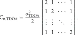
Figure 1shows the mean square range errors (MSREs) of the TOA-based CWLS and NLS estimators as well as CRLB versus power of distance error based on the TOA measure-ments. For simplicity, we assumed that the disturbances in the TOA measurements, namely,{nTOA,i}, were white
Gaus-sian processes with identical variances. The MSRE was de-fined asE[(x−x)2+ (y−y)2] and its unit was m2, which be-came dBm2in dB scale. We observe that the performance of the proposed and NLS methods met the CRLB when the TOA noise power was less than 75 dBm2and 60 dBm2, respectively, which indicated that the former had a larger optimum oper-ation range. The effect of positive mean TOA errors, which corresponded to NLOS propagation, was also illustrated in the same figure. Here the range measurements were modeled as
rTOA,i=di+nTOA,i+Nui, (103)
whereN = 100 m was the maximum error introduced by NLOS andui,i = 1, 2,. . .,M, were independent uniformly
distributed random numbers ranged from 0 to 1. It is seen that the nonzero mean errors introduced biases in both
methods when the TOA noise power was less than 35 dBm2, but its effect became negligible for larger power ofnTOA,i,
par-ticularly for the CWLS estimator.
Figures2,3, and4 show the MSREs of the RSS-based, TDOA-based, and AOA-based positioning algorithms, re-spectively, as well as the corresponding CRLBs, versus power of measurement errors. The disturbances in the RSS and AOA measurements were white Gaussian processes with identical variances as in the TOA measurements. As the units of theσ2
RSS,iandσAOA,2 iwere m2aand rad2, they became dBm2a
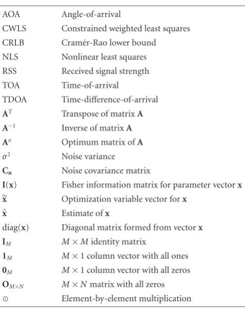
and dBrad2when represented in dB scales. While the TDOA measurements were Gaussian with covariance matrix of the form
Cn,TDOA=σ 2 TDOA
2
⎡ ⎢ ⎢ ⎢ ⎢ ⎢ ⎢ ⎣
2 1 · · · 1 1 2 · · · 1 ..
. ... . .. ... 1 1 · · · 2
⎤ ⎥ ⎥ ⎥ ⎥ ⎥ ⎥ ⎦
. (104)
From the figures, we observe that the performance of all the proposed methods approached the corresponding CRLBs for sufficiently small measurement errors, which verified their optimality at sufficiently high SNRs. Moreover, the superi-ority of the CWLS approach over the NLS scheme was again demonstrated for larger disturbance environments.
Figure 5shows the MSREs with TDOA-AOA hybrid surements, where the disturbances in the same type of mea-surements had identical power with zero mean, and they were uncorrelated with each other. It can be observed that the variances of the CWLS estimator approached the corre-sponding CRLB for all cases while the NLS scheme failed to produce optimum performance particularly when the AOA noise power was−10 dBrad2. This illustrated that the CWLS estimator for TDOA-AOA hybrid mobile positioning was op-timum for uncorrelated TDOA and AOA measurements and was more robust than the NLS method.
The computational complexity of the CWLS and NLS methods was also compared using the average number of floating point operations (FLOPS) provided by MATLAB, and the results are given inTable 2. It is seen that for AOA measurements, the proposed method required fewer FLOPS than the NLS while it needed more FLOPS for RSS and TOA measurements. For TDOA and TDOA-AOA hybrid measure-ments, both methods had comparable complexity. It is note-worthy to mention that the computational requirements of the CWLS approach can be significantly reduced if we only solve for the Lagrange multiplier whose value is closest to zero as in the LCLS method [15].
6. CONCLUSIONS
90 100 110 120 130 140 150 160 170 180 RSS noise power (dBm2a)
0 10 20 30 40 50 60 70 80 90 100
Me
an
sq
u
ar
e
ra
n
ge
er
ro
r
(d
B
m
2)
Proposed NLS
CRLB No. of BS=5, MS at [1000, 2000] m
Figure2: Mean square range errors for RSS measurements in un-correlated noise.
10 20 30 40 50 60 70 80 90 100
TDOA noise power (dBm2) 0
20 40 60 80 100 120 140
Me
an
sq
u
ar
e
ra
n
ge
er
ro
r
(d
B
m
2)
Proposed NLS
CRLB No. of BS=5, MS at [1000, 2000] m
Figure3: Mean square range errors for TDOA measurements in correlated noise.
then solved in an optimum manner with the use of weighted least squares and/or method of Lagrange multipliers. The proposed approach is quite flexible in that it can be easily extended to hybrid measurement cases such as the TDOA-AOA. We have proved that for small uncorrelated noise dis-turbances, the performance of all the proposed CWLS and WLS algorithms attains zero bias and the Cram´er-Rao lower
−70 −60 −50 −40 −30 −20 −10 0 10 20 AOA noise power (dBrad2)
0 50 100 150
Me
an
sq
u
ar
e
ra
n
ge
er
ro
r
(d
B
m
2)
Proposed NLS
CRLB No. of BS=5, MS at [1000, 2000] m
Figure4: Mean square range errors for AOA measurements in un-correlated noise.
10 20 30 40 50 60 70
TDOA noise power (dBm2) 0
20 40 60 80 100 120 140
Me
an
sq
u
ar
e
ra
n
ge
er
ro
r
(d
B
m
2)
Proposed NLS
CRLB No. of BS=5, MS at [1000, 2000] m
AOA noise power= −10 dBrad2 AOA noise power= −40 dBrad2
AOA noise power= −70 dBrad2
Figure5: Mean square range errors for using both TDOA and AOA measurements.
Table2: Computational complexity of proposed and NLS methods in terms of FLOPS.
Proposed NLS
TOA 7125 1978
RSS 6991 1393
TDOA 9892 8058
AOA 1075 2667
TDOA-AOA 11464 11994
APPENDICES
A.
A.1. TDOA
Following [15], we differentiate (27) and equate the expres-sion to zero:
∂LTDOA(˘ϑ,η) ∂ϑ˘ =2
GTΥ−1G+ηΣϑ˘−2GTΥ−1h=0.
(A.1)
The solution to (A.1) is
ϑ=GTΥ−1G+ηΣ−1
GTΥ−1h, (A.2)
where ηis not yet determined. The Lagrange multiplier is then found by substituting (A.2) into the constraint (23):
hTΥ−1GGTΥ−1G+ηΣ−1ΣGTΥ−1G+ηΣ−1GTΥh=0. (A.3)
Using eigenvalue factorization, the matrixGTΥ−1GΣcan be diagonalized as
GTΥ−1GΣ=SDS−1, (A.4)
whereD=diag(ζ1,ζ2,ζ3) andζi,i=1, 2, 3, are the
eigenval-ues of the matrixGTΥ−1GΣ. Substituting (A.4) into (A.3), the constraint can be rewritten as
αTD+ηI
3
−2β
=0, (A.5)
whereα=STΣGTΥ−1h=[α1,α2,α3]Tandβ=S−1GTΥ−1h= [β1,β2,β3]T. Simplifying (A.5) gives (29).
A.2. RSS
The minimum of (44) is obtained by differentiatingLRSS( ˘θ, λ) with respect to ˘θand then equating the resultant expres-sions to zero:
∂LRSS( ˘θ,λ) ∂θ˘ =2
ATΨ−1A+λPθ˘−2ATΨ−1b+λq=0.
(A.6)
The solution to (A.6) is
θ=ATΨ−1A+λP−1
ATΨ−1b−λ 2q
, (A.7)
whereλis not determined yet. To findλ, we substitute (A.7) into the equality constraint of (36):
qTATΨ−1A+λP−1
ATΨ−1b−λ 2q
+
bTΨ−1A−λ 2q
T
×ATΨ−1A+λP−1PATΨ−1A+λP−1
×
ATΨ−1b−λ 2q
=0.
(A.8)
Note that the matrix (ATΨ−1A)−1Pcan be diagonalized as
ATΨ−1A−1P=UΛU−1, (A.9)
whereΛ =diag(γ1,γ2,γ3), andγi,i=1, 2, 3, are the
eigen-values of the matrix (ATΨ−1A)−1P. Substituting (A.9) into (ATΨ−1A+λP)−1gives
ATΨ−1A+λP−1=
UI3+λΛ
−1
U−1ATΨ−1A−1 . (A.10)
Putting (A.10) into (A.8), we get
cTI3+λΛ
−1
f−λ
2c
TI
3+λΛ
−1
g
+eTI
3+λΛ
−1Λ
I3+λΛ
−1
f
−λ 2e
TI
3+λΛ
−1Λ
I3+λΛ
−1
g
−λ 2c
TI
3+λΛ
−1Λ
I3+λΛ
−1
f
+λ 2
4c
TI
3+λΛ
−1Λ
I3+λΛ)−1g=0,
(A.11)
where
cT=qTU=c1,c2,c3,
g=U−1ATΨ−1A−1q=g1,g2,g3T,
eT=bTΨ−1AU=e1,e2,e3,
f=U−1ATΨ−1A−1ATΨ−1b=f1,f2,f3T.