Frequency and 2D Angle Estimation Based on a Sparse Uniform Array of Electromagnetic Vector Sensors

(1)

Volume 2006, Article ID 80720, Pages1–9 DOI 10.1155/ASP/2006/80720

Frequency and 2D Angle Estimation Based on

a Sparse Uniform Array of Electromagnetic

Vector Sensors

Fei Ji1_{and Sam Kwong}2

1_{School of Electronic and Information Engineering, South China University of Technology, Guangzhou 510640, China} 2_{Department of Computer Science, City University of Hong Kong, Tat Chee Avenue, Kowloon, Hong Kong}

Received 25 April 2005; Revised 25 January 2006; Accepted 29 January 2006

Recommended for Publication by Joe C. Chen

We present an ESPRIT-based algorithm that yields extended-aperture two-dimensional (2D) arrival angle and carrier frequency estimates with a sparse uniform array of electromagnetic vector sensors. The ESPRIT-based frequency estimates are first achieved by using the temporal invariance structure out of the two time-delayed sets of data collected from vector sensor array. Each incident source’s coarse direction of arrival (DOA) estimation is then obtained through the Poynting vector estimates (using a vector cross-product estimator). The frequency and coarse angle estimate results are used jointly to disambiguate the cyclic phase ambiguities in ESPRIT’s eigenvalues when the intervector sensor spacing exceeds a half wavelength. Monte Carlo simulation results verified the eﬀectiveness of the proposed method.

1. INTRODUCTION

The localization of source signals using vector sensor data processing has attracted significant attentions lately. Many advantages of using the vector sensor array have been identi-fied and many array data processing techniques for source localization and polarization estimation using vector sen-sors have been developed. Nehorai and Paldi developed the Cram´er-Rao bound (CRB) and the vector cross-product DOA estimator using the vector cross product of the

electric-field and the magnetic-electric-field vector estimates [1,2]. Li [3]

de-veloped ESPRIT-based angle and polarization estimation al-gorithm using an arbitrary array with small loops and short dipoles. Identifiablity and uniqueness study associated with

vector sensors were done by Hochwald and Nehorai [4], Ho

et al.[5] and Tan et al. [6]. Hochwald and Nehorai [7]

stud-ied parameter estimations with application to remote sensing

by vector sensors. Ho et al. [8] developed a high-resolution

ESPRIT-based method for estimating the DOA of partially

polarized sources. Ho et al. [9] further studied the DOA

es-timation with vector sensors for scenarios where completely

and incompletely polarized signals may coexist. Wong [10]

has showed that the vector cross-product DOA estimator re-mains fully applicable for a pair of dipole triad and loop triad spatially displaced by an arbitrary and unknown distance

(rather than being collocated). Uni-vector-sensor ESPRIT is first presented to estimate 2D DOA and the polariza-tion states of multiple monochromatic noncoherent incident sources using a single electromagnetic vector sensor by Wong

and Zoltowski [11]. Nehorai and Tichavsky [12] presented an

adaptive cross-product algorithm for tracking the direction to a moving source using an electromagnetic vector sensor.

Ko et al. [13] proposed a structure for adaptively separating,

enhancing, and tracking up to three uncorrelated broadband

sources with an electromagnetic vector sensor. Wong [14]

proposed an ESPRIT-based adaptive geo-location and blind interference rejection scheme for multiple noncooperative wideband fast frequency-hop signals using one electromag-netic vector sensor. The maximum likelihood (ML) and min-imum variance distortionless response (MVDR) estimators for signal DOA and polarization parameters for correlated

sources are derived by Rahamim et al. [15]. In addition,

a novel preprocessing method based on the polarization smoothing algorithm (PSA) for “decorrelating” the signals

was also presented. Wong and Zoltowski [16] presented a

(2)

arrival angles from the estimation of the sources’ polarization parameters. The same authors further developed a closed-form direction-finding algorithm applicable to multiple ar-bitrarily spaced vector sensors at possibly unknown

loca-tions [17]. A sparse uniform array suﬀers cyclic ambiguity

in its direction-cosine estimates due to the spatial Nyquist sampling theorem. Zoltowski and Wong then further pre-sented another novel ESPRIT-based 2D arrival angle estima-tion scheme to resolve the aforemenestima-tioned ambiguity and achieve aperture extension for a sparse uniform array of vec-tor sensors spaced much further apart than a half wavelength

[18]. An improved version of the disambiguation algorithm

is also presented in [19].

In fact, frequency estimation is a fundamental problem in estimation theory and its applications include radar, ar-ray signal processing, and frequency synchronization. For scalar sensor array, a number of ESPRIT-based angle and fre-quency estimation methods have been proposed. Lemma et al. presented joint angle-frequency estimation method using multidimensional and multiresolution ESPRIT algorithms

[20,21]. Zoltowaki and Mathews discuss ESPRIT-based

real-time angle-frequency estimation algorithm using scalar

sen-sor array [22].

In this paper, we try to combine the ESPRIT-based frequency estimation with Wong’s ESPRIT-based 2D DOA

estimation scheme in [18] to yield extended-aperture

two-dimensional (2D) arrival angle and carrier frequency esti-mates with a sparse uniform array of electromagnetic vector sensors. Most of the works mentioned above have previously proposed direction-finding and polarization estimation al-gorithms using electromagnetic vector sensors; however, this paper is the first in advancing an algorithm for the estimation of both arrival angles and arrival delays.

In the newly proposed algorithm, the ESPRIT-based fre-quency estimates are achieved using the temporal invariance structure out of two time-delayed sets of data collected from vector sensor array. In that each incident source’s direction of arrival (DOA) coarse estimation is obtained through a vector cross-product estimator. Then the frequency estimates and coarse angle estimates results are used jointly to disambiguate the cyclic phase ambiguities in ESPRIT’s eigenvalues when the intervector sensor spacing exceeds a half wavelength.

2. MATHEMATICAL MODEL

Consider the scenario of K uncorrelated monochromatic

completely polarized transverse electromagnetic planewaves

signals with diﬀerent carrier frequencies, impinging on an

L-shaped array of regularly equally spaced and identical

elec-tromagnetic vector sensors from directions (θ_k,φ_k) and

po-larization parameters (γk,ηk) (k = 1,. . .,K). 0 ≤ θk < π

is thekth signal’s elevation angle measured from verticalz

-axis, 0≤φk<2πis azimuth angle, 0≤γk < π/2 is auxiliary

polarization angle, and−π ≤ ηk < πis polarization phase

diﬀerence.

The signal source model is given by

sk(n)=Pkej(2π fkn+ϕk)_, _n₌_{1, 2,}_{. . .}_,_N_, ₍₁₎

where P_k is the kth source’s energy, ϕ_k is the kth signal’s

uniformly distributed random phase, andN is the number

of independent samples collected by the array. fkis thekth

source’s digital frequency (between−0.5 and 0.5)

normal-ized to the sampling frequencyFswhich satisfies the Nyquist

sampling theorem for all the signals’ frequencies. Here we

normalize toF_s=1.

A vector sensor contains three electric and three mag-netic orthogonal sensors. The spatial response in matrix

no-tation of one vector sensor for the kth signal may be

ex-pressed as follows [11]:

gkdef= ⎡ ⎢ ⎢ ⎢ ⎢ ⎢ ⎢ ⎢ ⎢ ⎢ ⎣

exk eyk ezk hxk hyk hzk ⎤ ⎥ ⎥ ⎥ ⎥ ⎥ ⎥ ⎥ ⎥ ⎥ ⎦

def

=

⎡ ⎢ ⎢ ⎢ ⎢ ⎢ ⎢ ⎢ ⎢ ⎢ ⎢ ⎣

sinγ_kcosθ_kcosφ_kejηk₋_cosγ_k_sinφ_k

sinγkcosθksinφkejηk_{+ cos}γk_cosφk

−sinγksinθkejηk

−cosγkcosθkcosφk−sinγksinφkejηk

−cosγkcosθksinφk+ sinγkcosφkejηk

cosγ_ksinθ_k

⎤ ⎥ ⎥ ⎥ ⎥ ⎥ ⎥ ⎥ ⎥ ⎥ ⎥ ⎦ .

(2)

Note thatg_k does not depend on the signal frequency.

e_kdef= [exk,eyk,ezk]T andh_kdef=[hxk,hyk,hzk]T (where the

su-perscript T denotes the vector transpose operator) are

or-thogonal to each other and the source’s direction of

propaga-tion, that is, the normalized Poynting vectorpk[18],

p_k=

⎡ ⎢ ⎣pxkpyk

pzk ⎤ ⎥ ⎦=ek

e_k × h∗_k

_h_k =

⎡ ⎢ ⎣ukvk

wk ⎤ ⎥ ⎦=

⎡ ⎢ ⎣

sin_θ_kcosφk

sinθksinφk

cosθk

⎤ ⎥ ⎦,

(3)

where∗denotes complex conjugation andu_k,v_k,w_k,

respec-tively, symbolize the direction cosine along thex-axis,y-axis,

and thez-axis.

The spatial phase factor of thekth signal at themth vector

sensor located (m−1)Δalongx-axis equals

qx

mθk,φkdef=ej2π fkFs(m−1)Δuk/c

=ej2π fkFs(m−1)Δsinθkcosφk/c_, m₌_{1, 2,}. . ._,M_,

(4)

wherecis the velocity of light. The spatial phase factor of the

kth signal at thelth vector sensor located (l−1)Δalongy-axis

equals

q_lyθk,φk=ej2π fkFs(l−1)Δvk/c

=ej2π fkFs(l−1)Δsinθksinφk/c_, l₌_{1, 2,}. . ._,L. (5)

The 6×1 vector measurement in thenth snapshot is

pro-duced by themth vector sensor alongx-axis and thelth

vec-tor sensor alongy-axis, respectively,

zx_m(n)=

K

k=1

gkqxmθk,φkSk(n) +nxm(n),

z_ly(n)=

K

k=1

gkq_lyθk,φkSk(n) +n_ly(n),

(3)

wherenx_m(n) andny_l(n), respectively, symbol 6×1

complex-valued zero-mean additive white noise vector innth snapshot

at themth vector sensor alongx-axis and thelth vector sensor

alongy-axis.

Time-delayed data collected from the linear vector sensor

array alongx-axis is

zx_mn+n0

=K

k=1

gkqx_mθk,φkSkn+n0

+nx_mn+n0

=K

k=1

g_kqx_mθ_k,φ_kS_k(n)ej2π fkn0₊_nx

mn+n0

,

(7)

wheren0is the constant sample delay.

We form the following matrices by using (6) and (7):

x1(n)=

zx₁(n),zx₂(n),. . .,zx_M₋₁(n)T=AS+N1,

y1(n)=

zx₂(n),zx₃(n),. . .,zx_M(n)T =AΦxS+N2,

x2(n)=

zy1(n),zy2(n),. . .,zyL−1(n) T₌

BS+N3,

y2(n)=

zy2(n),zy3(n),. . .,zyL(n)T =BΦyS+N4,

y3(n)=

zx₁n+n0

,zx₂n+n0

,. . .,zx_M₋₁n+n0 _T

=AΦtS+N5,

(8)

where

Sdef=

⎡ ⎢ ⎢ ⎣

S1(n) .. .

SK(n) ⎤ ⎥ ⎥

⎦, N1def= ⎡ ⎢ ⎢ ⎣

nx1(n) .. .

nx_M₋₁(n) ⎤ ⎥ ⎥ ⎦, N2 def = ⎡ ⎢ ⎢ ⎣

nx2(n) .. .

nx_M(n) ⎤ ⎥ ⎥

⎦, N3 def = ⎡ ⎢ ⎢ ⎣

n1y(n) .. .

n_Ly₋₁(n) ⎤ ⎥ ⎥ ⎦,

N4def= ⎡ ⎢ ⎢ ⎣

n2y(n) .. .

n_Ly(n) ⎤ ⎥ ⎥

⎦, N5def= ⎡ ⎢ ⎢ ⎣

nx1

n+n0

.. .

nx_M₋₁n+n0 ⎤ ⎥ ⎥ ⎦, (9)

A=ax1,. . .,axK

=qxθ1,φ1

⊗g1,. . .,qx

θK,φK⊗gK, (10)

B=ay1,. . .,aKy

=qyθ1,φ1

⊗g1,. . .,qy

θK,φK⊗gK, (11)

qxθk,φkdef=

⎡ ⎢ ⎢ ⎢ ⎢ ⎣ 1

ej2π fkFSΔuk/c

.. .

ej2π fkFS(M−2)Δuk/c

⎤ ⎥ ⎥ ⎥ ⎥ ⎦,

qyθk,φkdef=

⎡ ⎢ ⎢ ⎢ ⎢ ⎣ 1

ej2π fkFSΔvk/c

.. .

ej2π fkFS(L−2)Δvk/c

⎤ ⎥ ⎥ ⎥ ⎥ ⎦. (12)

AandBare the 6(M−1)×Kand 6(L−1)×Kmatrices,

respectively, and⊗denotes Kronecker product.Φx,Φy, and

Φt_{are diagonal}_K_×_K_{matrices and are given by}

Φx₌_diag_exp j2π f1FSΔu1

c ,. . ., exp

j2π f_KF_SΔu_K

c

,

Φy₌_diag_exp j2π f1FSΔv1

c ,. . ., exp

j2π f_KF_SΔv_K

c

,

Φt₌_diag_exp_j₂_{π f} 1n0

,. . ., expj2π f_Kn0

.

(13)

FromNsnapshots, three data sets are formed as the

follow-ing:

Z1= X1 Y1 =

x1(1) · · · x1(N)

y1(1) · · · y1(N)

,

Z2= X2 Y2 =

x2(1) · · · x2(N)

y2(1) · · · y2(N)

,

Z3= X1 Y3 =

x1(1) · · · x1

N−n0

y3(1) · · · y3

N−n0

.

(14)

The key problem now is how to estimate the digital

fre-quencies {fk}K_k₌₁ and arrival angles {θk,φk}K_k₌₁ from the

above data sets.

3. ESPRIT-BASED FREQUENCY AND 2D ANGLE

ESTIMATION ALGORITHM

From (14), we have formed three distinct matrix-pencil

pairs. This first matrix pencilX1andY1has a spatial

invari-ance along thex-axis and can yield estimates of the direction

cosines{uk,k=1,. . .,K}. This second matrix pencilX2and

Y2has a spatial invariance along they-axis and can yield

es-timates of the direction cosines{vk,k=1,. . .,K}. This third

matrix pencilX1andY3has a temporal invariance and can

yield estimates of the frequency{fk,k=1,. . .,K}.

The first step in ESPRIT is to compute the signal-subspace eigenvectors by eigendecomposing the data

corre-lation matricesR1 =Z1Z1H,R2 =Z2Z2H, andR3 =Z3Z3H

(where the superscriptHdenotes the vector conjugate

trans-pose operator). In the protrans-posed algorithm, we basically

mod-ified the algorithm proposed in [18]. Thus, steps 2 to 6 are

similar to and taken out from [18].

(1) Deriving the frequency estimates

LetEt_Sdenote the 12(M−1)×Ksignal-subspace

eigenvec-tor matrix whoseKcolumns are the 12(M−1)×1

signal-subspace eigenvectors associated with theKlargest

eigenval-ues ofR3=Z3Z3H.

The invariance structure of the matrix-pencil pair

im-pliesEt_Scan be decomposed into two 6(M−1)×Ksubarrays

such that [23]

Et_S=

Et1

Et2

=

ATt AΦtTt

. (15)

Because bothEt₁andEt₂are full rank, a unique

nonsingu-larK×KmatrixΨtexists such that [11]

Et1Ψt=Et2=⇒ATtΨt=AΦtTt

=⇒Ψt₌_Tt−1_Φ_t

(4)

Ψt _{can be estimated by the total-least-squares ESPRIT}

covariance algorithm (TLS-ESPRIT) [23].

Ψt_{’s eigenvalues equal}_{_[_Φt_]_kk₌_ej2π fkn0_,k₌_1,. . ._,K_}_,

expj2πfkn 0

=Φt

kk. (17)

If the maximum of the signal digital frequencies is fmax,

n0is chosen as the following:

₂_{π f}_max_n₀_≤_π_=⇒_n₀_≤ 1

2fmax.

(18)

Then we can get the unambiguous frequency estimates:

fk=arg

Φt

kk

2πn0

, (19)

where arg{z}is principle argument of the complex number

zbetween−πandπ.

(2) Deriving the low-variance but ambiguous estimates ofuk

Similarly, for the matrix pencil pair with spatial

invari-ance along the x-axis, Ψx’s eigenvalues equal {[Φx]_kk =

ej2π fkFSΔuk/c_, k₌_1,. . ._,K_}_.

BecauseΔ≥λk(k = 1,. . .,K) and−1 ≤uk ≤1, there

exists a set of cyclically related candidates for the estimation

ofuk[18]:

uknu=μk+ nuc fkFSΔ

,

fkFSΔ

c

−1−μk≤nu≤ fkFSΔ

c

−1−μk,

μk=

argΦx_kk·c

2πfkFS Δ ,

(20)

wherexis the smallest integer not less thanx; xis the

largest integer not greater thanx.

(3) Deriving the low-variance but ambiguous estimates ofvk

Similarly, for the matrix pencil pair with spatial

invari-ance along the y-axis, Ψy’s eigenvalues equal {[Φy]_kk =

ej2π fkFsΔvk/c_,k₌_1,. . ._,K_}_.

There exists a set of cyclically related candidates for the

estimation ofvk[18]:

vknv=vk+ nvc fkFSΔ,

fkFSΔ

c

−1−vk≤nv≤ fkFSΔ

c

1−vk,

vk=arg

Φy

kk

·c

2πfkFS Δ .

(21)

(4) Deriving the unambiguous coarse reference estimates ofu_kandv_kfrom ESPRIT’s eigenvector

Ψx_{’s right eigenvectors constitute the columns of}_Tx_{. From}

[11], we have the following:

A=0.5Ex₁Tx−1+Ex₂Tx−1Φx−1. (22)

With noise, the above estimation becomes only approxi-mate.

We have the array manifold estimates from (10):

ax_k=qxθk,φk⊗g_k=qxθk,φk⊗

ek

hk

=

⎡ ⎢ ⎢ ⎢ ⎢ ⎢ ⎢ ⎢ ⎣

qx

1

θk,φkek

qx 1

θk,φkhk

.. . qx

M−1

θk,φkek

qx M−1

θk,φkhk ⎤ ⎥ ⎥ ⎥ ⎥ ⎥ ⎥ ⎥ ⎦ .

(23)

Define

bi(k)=q_ixθk,φkek, ci(k)=qx_iθk,φkhk, (24)

i=1, 2,. . .,M−1.

Note that

bi(k)

_b_i₍_k₎ ×c∗i (k)

ci(k) =

qx

iθk,φkek _qx

i

θk,φkek × qx∗

i θk,φkh∗k _qx

iθk,φkhk

=ek

e_k

h∗_k

hk .

(25)

So we can get the estimate of Ponyting vector:

px_k=_M1₋

1

M−1

i=1

b_i(k) b_i(k) ×

c∗_i (k)

c_i(k) . (26)

Unambiguous but high-variance estimates{px

xk,pxyk,pxzk}

for{uk,vk,wk}have been achieved. This is the so-called

vec-tor cross-product estimavec-tor who is pioneered by Nehorai

and Paldi [1,2] and firstly adapted to ESPRIT by Wong and

Zoltowski [11,24].

Similarly, for the matrix pencil with spatial invariance

along they-axis, we can get another set of unambiguous but

high-variance estimates p_ky for{uk,vk,wk}. For the matrix

pencil with temporal invariance, we can getpt_k.

(5) Pairing the direction-cosine estimates and frequency estimates

The orderings of{pt

xi,ptyi,ptzi, i=1, 2,. . .,K},{px jx,pxy j,pxz j,

j=1, 2,. . .,K}and{p_xky,p_yky ,p_zky,k=1, 2,. . .,K}are diﬀ

er-ent and need to be paired.{pt

(5)

with{px

x j,pxy j,pz jx}and{pxky,pyky ,pzky}as follows [18]:

j0

1,. . .,jK0

=arg min pt₁,. . .,pt_K−px_j1,. . .,px_j_K ,

k0

1,. . .,kK0

=arg min pt1,. . .,ptK

−p_k1y,. . .,p_ky_K .

(27) The above minimization is with respect to all possible

per-mutations of{k1,. . .,kK}and{j1,. . .,jK}.

Frompt_k,px_k,p_kywe may form ap_k:

p_k=

⎡ ⎢ ⎣ pxk pyk

pzk

⎤ ⎥

⎦= ptk+pxk+p

y k

3 . (28)

{pt

xi,ptyi,ptzi} are already paired with fi, and {pxx j,pxy j,

px

z j}withμj,{pyxk,pyyk,pzky}withvk. It follows that{f1,. . .,

fK}is to be paired with{μj0

1,. . .,μj0K}and{vk10,. . .,vk0K}[18].

(6) Disambiguation of the low-variance estimates of direction-cosine from ESPRIT’s eigenvalues [18]

The disambiguated estimates are

uknu=μk+ n ◦ uc

fkFSΔ, vk

nv=vk+ n ◦ vc

fkFSΔ, (29)

wheren◦_uandn◦_vmay be separately estimated as

n◦

u=arg min

nu

pxk−μk− nuc

fkFSΔ ,

n◦

v=arg min

nv

pyk−vk− nvc

fkFSΔ

.

(30)

(7) The 2D arrival angle estimation

We can calculate low-variance 2D arrival angle estimates from direction-cosine estimates out of ESPRIT’s eigenvalues

θk=arcsinu2

k+v2k

,

φk=arctan vk

uk

!

. (31)

Similarly, we can calculate the high-variance 2D arrival angle estimates from direction-cosine estimates out of ES-PRIT’s eigenvectors

θk=arcsin

p2

xk+p2yk

,

φk=arctan pyk

pxk

!

. (32)

Note thatp_zkmay be applied to judge the quadrant ofθ_k.

4. SIMULATIONS

Several simulations are presented to verify the eﬀectiveness of

the proposed ESPRIT-based frequency and 2D angle estima-tion algorithm. In these simulaestima-tions, the total-least-squares

10−5 10−4 10−3 10−2 10−1 100

RMS

standar

d

de

vi

ation

o

f

ang

le

estimat

es

(r

ad)

−10 −5 0 5 10 15 20 25 30

SNR (dB) CRB

From eigenvalue combined with eigenvectors From only eigenvectors

Figure1: The RMS standard deviation of (θk,φk, k=1, 2) versus SNR: the two uncorrelated sources{θ1,θ2} =(30◦, 60◦),{φ1,φ2} = (40◦,−60◦_), _{_γ

1,γ2} = (0◦, 45◦), {η1,η2} = (0◦, 90◦),{f1,f2} = (0.3, 0.4) impinge upon anL-shaped vector sensor, 100 snapshots per experiment, 300 experiments per data point.

10−6 10−5 10−4 10−3 10−2 10−1

RMS

standar

d

de

vi

ation

o

f

fr

eq

u

ency

estimat

es

−10 −5 0 5 10 15 20 25 30

SNR (dB) CRB

Frequency estimates

Figure2: The RMS standard deviation of (fk,k=1, 2) versus SNR,

same settings as anFigure 1.

ESPRIT covariance algorithm (TLS-ESPRIT) [23] is used.

We consider the scenario of the two signals impinging one

uniformL-shaped array andM = 4,L = 4. All the signal

source’s energyPis unity andn0=1. The intersensor

spac-ing is chosen asΔ=10∗λmin/2 (λmin=c/(fmaxFs)) except

for the example in Figures4and5.

Figures1and2give the RMS standard deviations of (θk,

(6)

10−7 10−6 10−5 10−4 10−3 10−2 10−1 100

RMS

bias

−10 −5 0 5 10 15 20 25 30

SNR (dB)

Angle estimates from eigenvalue combined with eigenvectors (rad)

Angle estimates from only eigenvectors (rad) Frequency estimates

Figure3: The RMS bias of (θk,φk, k = 1, 2) and (fk, k = 1, 2)

versus SNR, same settings as inFigure 1.

parameters of the two signals are{θ1,θ2} =(30◦, 60◦),{φ1,

φ2} =(40◦,−60◦),{γ1,γ2} =(0◦, 45◦),{η1,η2} =(0◦, 90◦),

{f1,f2} = (0.3, 0.4).Figure 3gives the corresponding RMS bias versus SNR. The proposed algorithm successfully re-solves all the two electromagnetic source parameters

includ-ing frequency and 2D angles. Figures1and3show that the

angle estimates from ESPRIT’s eigenvalues combined with eigenvectors have better performance than angle estimates obtained from only ESPRIT’s eigenvectors at SNR’s above 1 dB. It is observed that the RMS bias of angle estimates is

less than 0.2◦ at SNR’s above 5 dB and 0.1◦ at SNR’s above

10 dB. RMS standard deviation of frequency estimates is less than one order of magnitude greater than the CRB at SNR’s above 0 dB.

Figures4and5, respectively, give the RMS standard

de-viations and bias of (θk,φk, k = 1, 2) versus intersensor

spacing when SNR = 15. The parameters of the two

sig-nals are {θ1,θ2} = (60◦, 30◦), {φ1,φ2} = (40◦,−60◦),

{γ1,γ2} =(0◦, 45◦),{η1,η2} =(0◦, 90◦),{f1,f2} =(0.4, 0.5). Figure 3shows that the standard deviations and bias of an-gle estimates from the eigenvalues combined with

eigenvec-tors decrease as the intersensor spacing increases whenΔ<

60λmin/2. But the performance of angle estimates obtained

from only the eigenvectors remains relatively constant as the

inter-sensor spacing increases. Note that whenΔ≥60λmin/2,

the standard deviations and bias of angle estimates from the eigenvalues combined with eigenvectors begin to increase as the intersensor spacing increases. In fact, this phenomenon

has been explained in [18].

From (29), it can be seen that the performance of

fre-quency estimation may aﬀect the performance of

low-var-iance angle estimation.Figure 6gives the RMS standard

devi-ation of (θk,φk,k=1, 2) versus SNR. The signal parameters

10−5 10−4 10−3 10−2 10−1

RMS

standar

d

de

vi

ation

o

f

ang

le

estimat

es

(r

ad)

100 ₁₀1 ₁₀2

Intersensor space (λmin/2) CRB

From eigenvalue combined with eigenvectors From only eigenvectors

Figure4: The RMS standard deviation of (θk,φk, k =1, 2) ver-sus intersensor spacing when SNR =15 dB: the two uncorrelated sources{θ1,θ2} = (60◦, 30◦),{φ1,φ2} = (40◦,−60◦),{γ1,γ2} = (0◦, 45◦),{η1,η2} =(0◦, 90◦),{f1,f2} =(0.4, 0.5) impinge upon an

L-shaped vector sensor, 100 snapshots per experiment, 300 experi-ments per data point.

10−5 10−4 10−3 10−2

RMS

bias

of

ang

le

estimat

es

(r

ad)

100 ₁₀1 ₁₀2

Intersensor space (λmin/2) From eigenvalue combined with eigenvectors From only eigenvectors

Figure5: The RMS bias of (θk,φk,k=1, 2) versus intersensor

spac-ing when SNR=15 dB, same settings as inFigure 4.

are the same as inFigure 1except that{f1,f2} =(0.35, 0.4).

(7)

10−5 10−4 10−3 10−2 10−1 100

RMS

standar

d

de

vi

ation

o

f

ang

le

estimat

es

(r

ad)

−10 −5 0 5 10 15 20 25 30

SNR (dB) CRB

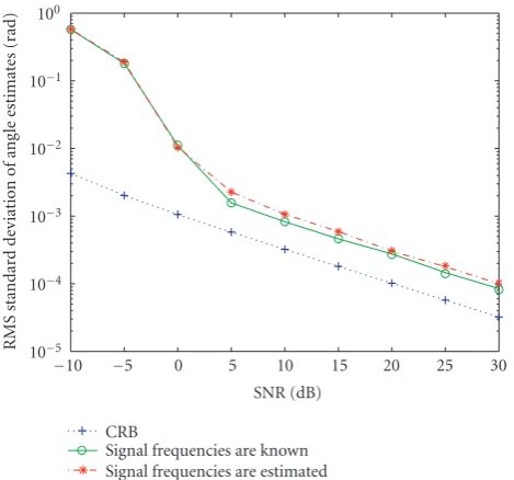
Signal frequencies are known Signal frequencies are estimated

Figure6: The RMS standard deviations of (θk,φk, k =1, 2) ver-sus SNR from low-variance angle estimation, same settings as in

Figure 1except that{f1,f2} =(0.35, 0.4).

just slightly lower than that when signal frequencies are esti-mated. Our simulations also show that RMS bias of the low-variance angle estimates when frequencies are known is al-most the same as that when frequencies are estimated.

Figure 7gives the RMS standard deviation of (θk,φk,k=

1, 2) versus elevation angle of the first signal when SNR =

15 dB. The parameters of the two signals areθ2=45◦,{φ1,

φ2} =(25◦,−30◦),{γ1,γ2} =(0◦, 45◦),{η1,η2} =(0◦, 90◦),

{f1,f2} = (0.3, 0.4). It is observed that the standard

devia-tions of angle estimates from the eigenvalues combined with eigenvectors are greater than angle estimates from ESPRIT

eigenvectors when elevation angle nears 90◦.

Figure 8gives the RMS standard deviation of (θ_k,φ_k,k=

1, 2) versus azimuth angle of the first signal when SNR =

15 dB. The signal parameters are the same as inFigure 7

ex-cept that{θ1,θ2} = (30◦, 45◦),φ2 = −30◦. It is shown that

the RMS standard deviation of angle estimates from two esti-mation methods almost does not change as the azimuth an-gle of the first signal is changed.

Figure 9gives the RMS standard deviation of (θk,φk,k=

1, 2) and (fk, k = 1, 2) versus the number of snapshots

when SNR = 15 dB. The parameters of the two signals are

{θ1,θ2} = (60◦, 30◦), {φ1,φ2} = (40◦,−60◦), {γ1,γ2} =

(0◦, 45◦), {η1,η2} = (0◦, 90◦), {f1,f2} = (0.3, 0.4). It is

shown that the RMS standard deviation decreases slowly as the number of snapshots increases for the number of snap-shots exceeding 50.

Figure 10gives the RMS standard deviation and bias of

(fk, k = 1, 2) versus the diﬀerence Δf of two signal

fre-quencies when SNR=15 dB. The signal parameters are the

same as inFigure 9 except that{f1,f2} = (0.4−Δf, 0.4).

10−4 10−3 10−2 10−1

RMS

standar

d

de

vi

ation

o

f

ang

le

estimat

es

(r

ad)

0 10 20 30 40 50 60 70 80 90

Elevation angle of the first signal (deg) From eigenvalue combined with eigenvectors From only eigenvectors

Figure7: The RMS standard deviations of (θk,φk, k =1, 2)

ver-sus elevation angle of the first signal when SNR =15 dB. The pa-rameters of the two signals areθ2 =45◦,{φ1,φ2} =(25◦,−30◦), {γ1,γ2} =(0◦, 45◦),{η1,η2} =(0◦, 90◦),{f1,f2} =(0.3, 0.4), 100 snapshots per experiment, 300 experiments per data point.

10−4 10−3 10−2 10−1

RMS

standar

d

de

vi

ation

o

f

ang

le

estimat

es

(r

ad)

0 10 20 30 40 50 60 70 80 90

Azimuth angle of the first signal (deg) From eigenvalue combined with eigenvectors From only eigenvectors

Figure8: The RMS standard deviation of (θk,φk, k=1, 2) versus

azimuth angle of the first signal when SNR=15 dB, same setting as inFigure 7except that{θ1,θ2} =(30◦, 45◦) andφ2= −30◦.

It is observed that whenΔf is 0.004, the RMS bias is about

2.5e-4 and standard deviation is about 1.6e-3, which shows that two signal frequencies can be separated. Note that just 50 snapshots are used here. For discrete Fourier transform when 50 snapshots are used, the frequency discrimination is

(8)

10−5 10−4 10−3 10−2 10−1

RMS

standar

d

de

vi

ation

0 100 200 300 400 500 600

Number of snapshots

Angle estimates from eigenvalue combined with eigenvectors (rad)

Angle estimates from only eigenvectors (rad) Frequency estimates

Figure9: The RMS standard deviation of (θk,φk, k = 1, 2) and

(fk, k = 1, 2) versus the number of snapshots when SNR =

15 dB. The parameters of the two signals are{θ1,θ2} =(60◦, 30◦), {φ1,φ2} = (40◦,−60◦),{γ1,γ2} = (0◦, 45◦),{η1,η2} = (0◦, 90◦), {f1,f2} = (0.3, 0.4), 100 snapshots per experiment, 300 experi-ments per data point.

10−6 10−5 10−4 10−3 10−2 10−1 100

10−3 ₁₀−2 ₁₀−1

Diﬀerence of two signal frequencies RMS standard deviation

RMS bias

Figure10: The RMS standard deviations and bias of (fk, k=1, 2)

versus the diﬀerenceΔf of two signal frequencies when SNR = 15 dB, same settings as inFigure 9except that {f1,f2} = (0.4−

Δf, 0.4), 50 snapshots per experiment, 300 experiments per data point.

5. CONCLUSION

In this paper, we propose an ESPRIT-based algorithm that yields 2D angle and frequency estimates. This algorithm can

achieve extended-aperture arrival angle estimation even though using a sparse electromagnetic vector sensor array. Good frequency discrimination obtained even though there

are little samples used. Although we only consider the L

-shaped array here, the approach may be implemented using a variety of array geometries.

ACKNOWLEDGMENTS

This work is supported by City University of Hong Kong Strategic Grant 7001697. This work is done when Fei Ji was visiting City University of Hong Kong.

REFERENCES

[1] A. Nehorai and E. Paldi, “Vector sensor processing for electro-magnetic source localization,” inProceedings of the 25th Asilo-mar Conference on Signals, Systems and Computers, vol. 1, pp. 566–572, Pacific Grove, Calif, USA, November 1991.

[2] A. Nehorai and E. Paldi, “Vector-sensor array processing for electromagnetic source localization,”IEEE Transactions on Sig-nal Processing, vol. 42, no. 2, pp. 376–398, 1994.

[3] J. Li, “Direction and polarization estimation using arrays with small loops and short dipoles,”IEEE Transactions on Antennas and Propagation, vol. 41, no. 3, pp. 379–386, 1993.

[4] B. Hochwald and A. Nehorai, “Identifiability in array pro-cessing models with vector-sensor applications,”IEEE Trans-actions on Signal Processing, vol. 44, no. 1, pp. 83–95, 1996. [5] K.-C. Ho, K.-C. Tan, and W. Ser, “Investigation on

num-ber of signals whose directions-of-arrival are uniquely deter-minable with an electromagnetic vector sensor,”Signal Pro-cessing, vol. 47, no. 1, pp. 41–54, 1995.

[6] K.-C. Tan, K.-C. Ho, and A. Nehorai, “Uniqueness study of measurements obtainable with arrays of electromagnetic vec-tor sensors,”IEEE Transactions on Signal Processing, vol. 44, no. 4, pp. 1036–1039, 1996.

[7] B. Hochwald and A. Nehorai, “Polarimetric modeling and pa-rameter estimation with applications to remote sensing,”IEEE Transactions on Signal Processing, vol. 43, no. 8, pp. 1923–1935, 1995.

[8] K.-C. Ho, K.-C. Tan, and B. T. G. Tan, “Eﬃcient method for estimating directions-of-arrival of partially polarized sig-nals with electromagnetic vector sensors,”IEEE Transactions on Signal Processing, vol. 45, no. 10, pp. 2485–2498, 1997. [9] K.-C. Ho, K.-C. Tan, and A. Nehorai, “Estimating directions of

arrival of completely and incompletely polarized signals with electromagnetic vector sensors,”IEEE Transactions on Signal Processing, vol. 47, no. 10, pp. 2845–2852, 1999.

[10] K. T. Wong, “Direction finding/polarization estimation— dipole and/or loop triads,”IEEE Transactions on Aerospace and Electronic Systems, vol. 37, no. 2, pp. 679–684, 2001.

[11] K. T. Wong and M. D. Zoltowski, “Uni-vector-sensor ESPRIT for multisource azimuth, elevation, and polarization estima-tion,”IEEE Transactions on Antennas and Propagation, vol. 45, no. 10, pp. 1467–1474, 1997.

[12] A. Nehorai and P. Tichavsky, “Cross-product algorithms for source tracking using an EM vector sensor,”IEEE Transactions on Signal Processing, vol. 47, no. 10, pp. 2863–2867, 1999. [13] C. C. Ko, J. Zhang, and A. Nehorai, “Separation and

(9)

[14] K. T. Wong, “Blind beamforming geolocation for wideband-FFHs with unknown hop-sequences,” IEEE Transactions on Aerospace and Electronic Systems, vol. 37, no. 1, pp. 65–76, 2001.

[15] D. Rahamim, J. Tabrikian, and R. Shavit, “Source localization using vector sensor array in a multipath environment,”IEEE Transactions on Signal Processing, vol. 52, no. 11, pp. 3096– 3103, 2004.

[16] K. T. Wong and M. D. Zoltowski, “Self-Initiating MUSIC-based direction finding and polarization estimation in spatio-polarizational beamspace,”IEEE Transactions on Antennas and Propagation, vol. 48, pp. 1235–1245, 2000.

[17] K. T. Wong and M. D. Zoltowski, “Closed-form direction finding and polarization estimation with arbitrarily spaced electromagnetic vector-sensors at unknown locations,”IEEE Transactions on Antennas and Propagation, vol. 48, no. 5, pp. 671–681, 2000.

[18] M. D. Zoltowski and K. T. Wong, “ESPRIT-based 2-D direc-tion finding with a sparse uniform array of electromagnetic vector sensors,”IEEE Transactions on Signal Processing, vol. 48, no. 8, pp. 2195–2204, 2000.

[19] M. D. Zoltowski and K. T. Wong, “Closed-form eigenstruc-ture-based direction finding using arbitrary but identical sub-arrays on a sparse uniform Cartesian array grid,”IEEE Trans-actions on Signal Processing, vol. 48, no. 8, pp. 2205–2210, 2000.

[20] A. N. Lemma, A. J. Van Der Veen, and E. F. Deprettere, “Anal-ysis of joint angle-frequency estimation using ESPRIT,”IEEE Transactions on Signal Processing, vol. 51, no. 5, pp. 1264–1283, 2003.

[21] A. N. Lemma, A. J. Van Der Veen, and E. F. Deprettere, “Joint angle-frequency estimation using multi-resolution ESPRIT,” inProceedings of IEEE International Conference on Acoustics, Speech and Signal Processing (ICASSP ’98), vol. 4, pp. 1957– 1960, Seattle, Wash, USA, May 1998.

[22] M. D. Zoltowski and C. P. Mathews, “Real-time frequency and 2-D angle estimation with sub-Nyquist spatio-temporal sam-pling,”IEEE Transactions on Signal Processing, vol. 42, no. 10, pp. 2781–2794, 1994.

[23] R. Roy and T. Kailath, “ESPRIT - estimation of signal param-eters via rotational invariance techniques,”IEEE Transactions on Acoustics, Speech, and Signal Processing, vol. 37, no. 7, pp. 984–995, 1989.

[24] K. T. Wong and M. D. Zoltowski, “High accuracy 2D angle es-timation with extended aperture vector sensor arrays,” in Pro-ceedings of IEEE International Conference on Acoustics, Speech and Signal Processing (ICASSP ’96), vol. 5, pp. 2789–2792, At-lanta, Ga, USA, May 1996.

Fei Ji received the B.S. degree from the Northwestern Polytechnical University in 1992 and the M.S. and Ph.D. degrees from South China University of Technol-ogy in 1995 and 1998. Upon graduation, she joined the Department of Electronic Engi-neering, South China University of Tech-nology in 1998 as a Lecturer. She worked in the City University of Hong Kong as a Research Assistant from March 2001 to July

2002 and a Senior Research Associate from January 2005 to March 2005. She is currently an Associate Professor in the School of Elec-tronic and Information Engineering, South China University of Technology.