Exploiting inter-conceptual relationships to boost SVM
classification
.Gert-Jan Poulisse
Acknowledgement ...iii
Chapter 1 Introduction ... 1
1.1 Goals ... 1
1.2 Approach ... 2
1.3 Organization of this paper ... 3
Chapter 2
Concept detection in literature ... 4
2.1 Related Works ... 4
2.2 Domain Based Classification ... 5
2.2 Statistical Based Classification ... 7
Chapter 3
Methodology ... 13
3.1 Basic terminology ... 13
3.2 Choosing a video annotation tool ... 13
3.3 Choosing a dataset ... 14
3.4 Choosing a Supervised learner ... 15
3.5 SVM in practice ... 15
3.6 Adjustment of the research approach ... 16
Chapter 4
Inter-conceptual boosting experiments ... 17
4.1 Experiment Setup ... 17
4.2 Experiment 1: Sibling-confusion removal ... 18
4.3 Sibling-confusion removal analysis ... 19
4.4 Experiment 2: Ancestor boosting ... 22
4.5 Ancestor boosting analysis ... 23
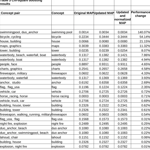
4.6 Experiment 3: Chi-Square boosting ... 25
4.7 Chi-Square explained ... 25
4.8 Chi-Square boosting analysis ... 27
4.9 Chi-square Conclusion ... 28
Chapter 5
Conclusion ... 30
References ... 32
Annex 1
SVM Theory ... 37
Annex 2
Sibling-confusion removal results ... 40
Annex 3
Ancestor boosting results ... 43
Abstract
Concept detection is the process of extracting semantic meaning from data. Video data is a popular choice on which to operate, as there is a lot of visual, audio, and textual information to index and search. Ultimately one would like to develop a set of semantic concepts that spans the search space, but this requires defining thousands of concepts. In order to detect such a copious amount of concepts, generic concept detectors have to be employed. There is a continuous drive in research to discover better ways to perform generic concept recognition.
This thesis starts with a literature overview, surveying past and future trends in concept detection. Past classification systems were often rule-based systems that made use of specific domain knowledge to perform their tasks. While functional, these systems could not readily be extended beyond their domain. State of the art classification systems on the other hand, use statistical models, in the form of Support Vector Machine classifiers, to recognize an unbounded set of concepts.
The initial thrust of this investigation was to examine the potential of using SVM classifiers to detect an abstract concept, such as ‘happiness’, by relating simpler, indicative concepts. This proved infeasible, and the focus of this research became to improve weak classifiers by exploiting the knowledge of more discernable, related classes. Three techniques were developed in this study that did this, each applicable to a different type of inter-conceptual relationship. This thesis aims to assess the performance and the associated constraints of these developed techniques.
The Sibling-confusion removal and Ancestor boosting techniques require an ontology, a tree-like structure that models semantic relationships between concepts by linking relationships in a hierarchy. The Sibling-confusion removal technique attempts to improve detector performance by removing false positives caused by similarities between sibling concepts. The Ancestor boosting technique aims to improve poorly performing child detectors by leveraging the functionality of their more powerful ancestor concept detectors.
The final technique used a statistical method, the chi-square test, to identify concepts in the dataset that frequently appeared simultaneously. Concept recognition was improved by combining the outputs from related detectors to recognize a single concept.
In the course of the experiments, a number of hidden constraints for each technique became apparent and explain the results thus obtained. Sibling-confusion removal proved to be a worthwhile technique when the ontology provides a concept grouping, which is semantically related, closed, and for which only one concept is valid in each shot. Ancestor boosting appears to be a promising technique, as evinced by substantial increase in detector performance for some concepts in the dataset. For Ancestor boosting to work successfully, however, it is necessary that ancestor and child concepts be tightly linked semantically and that ancestor detectors perform robustly. Chi-square boosting is a powerful technique, as it identifies concept relationships that are not immediately obvious from their semantic definitions. Most of the discovered concept relationships may be used to produce improved concept detectors.
Acknowledgement
I wish to recognize the considerable assistance afforded to the conduct of this research and preparation of the manuscript by Maarten Fokkinga, CS Department, Twente University. His particular ability to stimulate and direct my curiosity, essential for charting unknown SVM database classification waters, is most gratefully acknowledged. Thanks are also due to Robin Aly for his useful discussions when in search for solutions.
GJP,
Enschede, August 2007
Chapter 1
Introduction
When a person goes to a public library to look for a book, he first goes to the card catalogue and looks for a book in the category he desires within the catalogue. Thus he has a fuzzy idea of what he is looking for, in the sense that he knows a few key words to describe it. The catalogue is ordered so that the keywords will narrow his search until he finds what he is looking for. This assumes however, that each book has been previously indexed and placed within the catalogue. If one extends the metaphor to searching for video footage, one realizes that the audio, video, and text streams that make up the video recording must also somehow be indexed. This is complicated however by that fact that a human would index by providing a textual summation of the content. To a computer however, the video stream is merely a sequence of images, with each image being a set of colored points. This is known as the semantic gap.
Nonetheless, it is possible to train a computer to recognize low-level features, such as the colors of an image, and associate them with concepts. The implicit loss of data associated with indexing, plus the ill-defined nature of semantic concepts means that this process introduces error. In addition, most sophisticated concepts can only be recognized by the presence of simpler concepts. For example, a car-chase scene could only be recognized if previous classifiers have recognized multiple cars following each other at high speeds. The art then, is to map low-level features to a concept vocabulary that covers the human language that minimizes error and provide maximum concept coverage.
Early research focused on combining multimodal feature extractors in various ad-hoc approaches to identify specific concepts. Unfortunately, this does not scale well, as the combination of feature extractors is case specific. Thus one cannot use the same combination of feature extractors to recognize a different concept. More recent research, such as the TRECVID high-level feature extraction task, focuses on implementing a framework of generic concept detectors to define a vocabulary that spans the human language. This task can be done by defining each concept as a unique blend of constituent features, or defines the concept to be identified in terms of other concepts. The challenge is to find an optimal combination of feature vectors and classifiers; and concept detection to date remains wide open to further research.
1.1 Goals
The initial aim of this research was to utilize the semantic relationships between some basic concepts to develop a concept detector capable of recognizing an abstract concept like ‘happiness’ in a dataset. Such a detector proved infeasible, and the focus of this research became to develop methods to improve weak classifiers by exploiting the knowledge of more discernable, related concepts.
1.2 Approach
An initial literature study was performed in order to discern past and current trends in research with respect to semantic concept detection. This study revealed that SVM classifiers were the most promising classifiers to date, and so it was decided to detect an abstract concept, such as ‘happiness’, by relating simpler, indicative concepts using SVM. A preliminary investigation showed this was not possible given the limitations of the available datasets. Instead, three techniques, inspired by the previously discovered literature, were developed to validate the hypothesis.
An ontology was created that models semantic relationships between concepts by linking relationships in a hierarchy. Two techniques, Sibling-confusion removal and Ancestor boosting utilized this ontology. The Sibling-confusion removal technique attempts to improve detector performance by removing false positives caused by similarities between sibling concepts. The Ancestor boosting technique aims to improve poorly performing child detectors by leveraging the functionality of their more powerful ancestor concept detectors.
A final technique was developed that used the Chi-square test to identify concepts that frequently appeared simultaneously. Concept recognition was improved by combining the outputs from related detectors to recognize a single concept.
1.3 Organization of this paper
This paper is organized as follows:
Chapter 2, Concept detection in literature, discusses past and present research efforts in concept detection. The aim of this survey was to present various concept detection techniques, their comparative merits, and the applicability of these techniques in detecting a wider set of concepts. The trend in research is moving away from knowledge-based systems to generic concept classifiers afforded by Support Vector Machines.
Chapter 3, Methodology, describes various practical issues related to the choice of supervised learner, annotation software, and dataset. In conjunction with some preliminary findings, these choices affected a change in the method of approach.
Chapter 4, Inter-conceptual boosting experiments, describes three techniques which aim to improve concept detector performance by using knowledge of the semantic and statistical concept relationships in a dataset. The Sibling-confusion removal technique attempts to improve detector performance by removing false positives caused by similarities between sibling concepts. The Ancestor boosting technique aims to improve poorly performing child detectors by leveraging the functionality of their more powerful ancestor concept detectors. In Chi-square boosting, concept recognition was improved by combining the outputs from related detectors to recognize a single concept. These techniques were evaluated on the MediaMill dataset, and their results are analyzed.
Chapter 5, Conclusion, discusses the conclusions of the paper and suggests further refinements in the techniques applied.
Annex 1, SVM Theory, presents a summarized mathematical background of Support Vector Machines and briefly introduces the parameter settings that influence the development of a SVM model.
Annex 2, confusion removal results, presents the results obtained using the Sibling-confusion removal technique developed in Chapter 4.
Annex 3, Ancestor boosting results, presents the results obtained using the Ancestor boosting technique developed in Chapter 4.
Chapter 2
Concept detection in literature
This chapter presents a review of a selection of papers, showing a chronological progression, documenting the progress made in research in the field of concept detection. The aim of this survey was to discover the various concept detection techniques used in research, their
comparative merits, and the applicability of these techniques in detecting a wider set of concepts. Some statistical classification systems and techniques presented here provide the basis for work done in chapter 4.
2.1 Related Works
For video data, there are three types input streams, the audio, video, and text (transcriptions of the words spoken in the segment). Feature extraction then, is the action of determining the characteristics for of the video fragment, in any of the three modalities, to detect some sort of concept. Some examples of features are: color histograms (indicative of the colors in the video), edge orientation histograms (represents the various edges of shapes in the video), Mel-frequency cepstrum coefficients (indicative of the rate of change of the audio), or word frequency (the number of occurrences of various words of (spoken) text). The process of combining these features in order to recognize a particular semantic concept is known as classification, or fusion.
Early research on semantic concept meta-classification examined ad-hoc rule based domain knowledge schemes, Bayesian classifiers (BN), neural network classification (NN), Gaussian mixture models(GMM), modeling via ontologies, Support Vector Machines(SVM), or Hidden Markov models(HMM). The various approaches are either statistical in nature (Bayesian, GMM, HMM, SVM), or are knowledge based, using knowledge of the domain (rule based, modeling using ontologies).
The drive to create a framework of detectors capable of recognizing generic concepts precludes the use of domain-based classifiers and is the reason for the trend towards statistical methods in research. This is not to say that domain based meta-classifiers perform poorly. Often they make use of insights, such as the dependency between two concepts, that short circuit the whole machine learning process of statistical methods, saving much development time. Their failure is in being unable to function properly for events outside their specific domain. For example, the highlights detection of Babaguchi [7] (discussed in 2.2) would fail for say, Formula 1. The reasoning behind using statistical classification is that enough features are considered that a concept is identified correctly, no matter the domain. In addition, the detection process as a whole is more robust, as more features are considered, and as such the error contribution per individual feature is lessened.
be performed in various ways, each with its own tradeoffs between extensibility, robustness, and the time spent on learning the semantic concepts.
Recent research shows a distinct preference for SVM classification, because it gives superior performance over other statistical approaches and because it is robust against overtraining and the curse of dimensionality[30]. For further understanding of the mathematical reasons for this, see Annex 1. Although some domain approaches are still attempted, statistical classification is now the trend. In the field of domain knowledge classifications, the work done on ontologies is a recent innovation. However, in this instance ontologies are often deployed on top of a generic classifier (such as SVM’s) to produce a hybrid attempting to incorporate domain knowledge on top of a statistical classifier.
Early research focused on developing ad-hoc concept recognition systems. They were rule-based, and operated on a fixed domain. These are reviewed in section 2.2. The desire to detect a much larger concept set led to the development of statistical concept detection methods, and are discussed in 2.3.
2.2 Domain Based Classification
Some of the first multimedia information retrieval systems to be developed investigated sports video. The system by Babaguchi and Nitta[7] was designed to analyze sports video, specifically baseball and American football, and determine the presence of semantic concepts such as highlights, live plays, crowd cheering, and the type of scene currently playing. Highlights were detected by examining the text stream for domain specific keyword phrases such as “touchdown” and then finding the corresponding time interval in the video stream. Crowd cheering was determined by the short time energy feature of the audio stream. Using the idea that crowd cheering was indicative of a highlight moments, a more sophisticated detector was developed by excluding highlights without cheering [7]. This system is an example of how specialized domain knowledge can readily provide a successful solution to identifying a specific semantic concept, such as highlights. The extensibility of the system is however open to question.
Haering et al [20], however, did develop a system seeking extensibility. The prototype system was designed to detect animal hunts in wildlife video, which is a complex semantic event. The promise of extensibility comes from the development of a modular, tiered system to allow easy redeployment for the detection of different semantic events. The first tier of the system extracted basic color, texture, and motion features, moving object blobs as well as shot boundary locations. Using these features, a neural network determined the class of the object under consideration. Nine of them were specific animals, five non-animals corresponding to rocks, sky/clouds, grass, trees, and a final unknown class. The third, and highest, tier of the system, in essence the meta-classifier, used domain specific rules to detect semantic events based on a combination of mid-level object descriptors spatially or temporally ordered based on the features from the first level.
Returning to concept detection in sports video, Xu [64] developed a somewhat domain (team-sport) independent system capable of handling semantic events which do not have significant audio/video features, such as when players are given yellow/red cards in soccer. He argues that most audio/video patterns are insufficiently distinct to recognize such semantic events. Likewise he argues that his system is readily extensible. His approach is to detect generic video concepts, using Hidden Markov Models (HMM), from the audio/video stream, such as shot category, focal distance, special view category, field zone, camera motion direction, and motion activity. Another HMM classifier is used to detect the transition between such events in the video stream. Domain dependencies are introduced in the form of external text streams detailing for instance game rules (important for field type and match duration), player names (facilitates text analysis), and event types (linking event types with AV patterns detected by the HMM), to detect more detailed semantic concepts. The assumption is that only noteworthy events are included in a match report.
Sports events defined in a text stream are aligned against previously detected generic video events, which constitute another classification problem. Xu compares three fusion methods, a rule-based scheme, a probabilistic aggregation scheme, and one using Bayesian inference that perform this alignment. The rule based scheme aligns text events within a temporal window based on the number of matches between text events and the externally provided, domain specific event model. Since text and video stream events are usually misaligned by some offset, the aggregation method models a semantic event as the combined probability of the event occurring in one stream and the probability of the event occurring in the other stream, offset by some margin. The margin is determined by gradient descent during a training phase. The last fusion method, Bayesian Inference, considers whether an event occurring in one stream occurs within a fixed offset in the other stream [64].
In terms of precision and recall, rule-based fusion gives the best performance, with Bayesian inference only mildly less accurate. Aggregation is the poorest performer [64]. All results have precision and recall above 84%. Xu attributes this discrepancy to sensitivity of the aggregation method and the large randomness in time offsets. The rule-based method benefits from using the additional detail possibly in the text stream and as such can correctly identify more events. The Bayesian Inference is unable to do so, and hence performs slightly worse. [64]
Xu’s system is a reasonably generic system for sports, with good precision and recall. There is support for extending the system, the only caveat being that every sport needs external, domain specific parameters. Xu argues that this data can often automatically be retrieved and parsed, whereas event models are non-volatile after construction. Provided there is some operator assistance to develop these models, the system can support a large number of sports. For increased performance, rule based fusion could be employed, requiring additional operator assistance to develop these alignment rules. For a slight drop in performance, but no requirement for human intervention, Baysian Inference would suffice.
2.3 Statistical Based Classification
The papers reviewed in this section perform classification using statistical methods, such as Hidden Markov models [1,2], Gaussian mixture models [1], or Support Vector Machines [1, 26, 30, 47, 55]. They are of interest because chronologically early papers contrast various classification methods, and determine that SVM gives superior classification performance [1, 26, 30, 47]. Later papers describe various methods to further improve SVM performance [26, 55, 62].
Alatan’s system [2] aims to detect dialogue scenes in video, and uses Hidden Markov Models (HMM) as the classifier. The dialogue scene, or story, is defined as a set of consecutive shots that make up a meaningful and distinct part of a whole story. An example of this would be a scene from a news broadcast. This would contain the shots of the news anchor introducing a news item, the news item itself, and possibly any concluding remarks made back in the studio. A scene is always present in video, irrespective the genre, and thus scene detection results in the partitioning of the video into semantically meaningful, logical units. What makes scene detection difficult is the absence of a fixed format to a scene. Care must be taken to neither miss shots that should be part of a scene, nor to accidentally subdivide a scene because of intermittent shots that break the visual flow (such as a close up) and yet are semantically relevant to the whole.
Alatan models a scene as consisting of three elements, people, conversation, and a location. People are detected using face detection, while audio is classified as either music, speech or silence. Shifts in location are detected by analyzing the histograms of several consecutive shots. The results of each detector are then used as inputs of an HMM to detect, and classify, scenes as either establishing, dialogue, or transitional, the three types most commonly used by film directors. He argues for HMM over rule-based, deterministic methods because HMM allow for random behavior, such as extraneous shots within a scene, as one might expect when analyzing video without any prior knowledge of the content. [2]
The use of a HMM classifier avoids the domain dependence of rule based classifiers, and can readily be made more robust by adding more classifiers as inputs. This would not however, require the alteration of the pre-existing classifiers. Likewise more semantic inferences, for example more distinct scene types, could be made by extending the output classification set of the particular HMM, although as with adding additional classifiers as inputs, each alteration requires the retraining of the HMM.
Snoek and Worring [47] also developed a system for use in the news and sports (soccer) domain. They propose a framework, called TIME, which is a multimodal approach to tackle the problems of context and time-synchronization common to these domains. This framework is evaluated using three statistical classifiers, C4.5 decision trees, Maximum Entropy, and SVMs. The choice for statistical classifiers was made in order to provide for a robust performance in domains such as soccer, where events are sparse, context dependent, and unpredictable.
C4.5 decision trees place these events into a binary tree based on a gain ratio determined at training time. Each concept is a leaf node in the tree, and the time-ordered events form decision nodes higher up in the tree. The more important the event is to the classification task, the higher it is in the tree [47]. A Maximum entropy (MaxEnt) classifier estimates the conditional distribution of a concept in a video, given certain constraints. These constraints are features, whose values are determined from the training set [47,68].
In the soccer domain, where concepts such {goal, yellow card, substitutions} concepts were looked for, C4.5 decision trees gave the poorest performance. MaxEnt and SVM detected all semantic concepts equally well. What differentiated them was that the SVM classifier required considerably less training time than the MaxEnt algorithm to achieve this result [47]. In the news domain, where concepts such as {reporting anchor, monologue, split-view interview, and weather-report} were sought, the SVM classifier outperformed the C4.5 and MaxEnt classifiers, both of whom performed similarly. In an additional experiment to test the effectiveness of the TIME framework, SVM based classification on the news domain was performed with temporal relations enabled and disabled. For most semantic concepts, the additional information provided by the TIME framework yielded increased performance, except for the weather report, where results were comparable [47].
The Time framework demonstrates that it is possible to add additional contextual information, in this case a temporal ordering, to low level concepts. This additional information results in better performance of the classifier than when it is not provided. This Time framework also suggests that SVM classifiers outperform C4.5 decision trees and MaxEnt classifiers over two different domains, and one could speculate that this would also apply for other domains.
One of the earliest applications of a SVM classifier was a 2002 system from Carnegie Mellon which integrated a video camera and two microphones in a tape-recorder like system. The video camera provided input to two face recognition detectors, while the microphones had feature detectors checking for speech identification by similarity and pitch. The purpose of the system was to remind the user of the last conversation, if any, had with a dialogue partner. The results clearly demonstrated that the individual detector results, or a summation of their results, resulted in a significantly poorer performance than when their outputs were fused using an SVM (late fusion) classifier [30].
IBM [1] has also focused research on multimedia retrieval. Rather than attempting a domain specific application, their system was explicitly designed to explore concept detection and the performance of various fusion schemes. Their system used machine learning over low level features on the audio, visual and text channels to determine the most effective model for various concepts. For all fusion methods however, late fusion was employed to combine unimodal features concept classification. Statistical classification, through the use of Support Vector Machines, and probabilistic modeling approaches, such as Gaussian Mixture Models (GMM), HMM, and Bayesian networks, were investigated. GMM and SVM performance was compared for visual features, while GMM and HMM performance was compared for fusion of audio features. The resultant concepts were considered unimodal, or atomic concepts. An investigation was made into the appropriate fusion model for high level concepts; concepts which can only be inferred by the presence of other concepts and low level features and are generally multimodal in nature. For this task, the performance of Bayesian networks was compared with a SVM classifier [1]. The video footage from the TREC 2001 corpus was used for evaluation.
recall range. Even with a small training set, SVM classifiers provided a reasonably accurate detection performance. [1]
For unimodal classification of audio features, which examined HMM versus GMM performance for the classification of {rocket engine explosion, music, speech, speech + music}, HMM precision outperformed GMM’s over all recall values [1]. These concepts were then used in an additional experiment examining the best fusion method to detect the semantic concept, ‘rocket launch’. Explicit fusion used the classification results from the previous unimodal classifiers as inputs into a Bayesian network to detect this concept. Implicit fusion uses the following function to generate a score for each concept:
F(ci) = f(c1…. cn) = Score(ci)/(Σ(Score(c1…cn)) where Score(ci) is the unimodal score for each concept in a shot.
Each concept is normalized by the sum of all the scores for concepts present in a given shot. For this particular concept, implicit fusion outperformed explicit fusion over all recall values. [1]
Although implicit outperformed explicit fusion, I would question the validity of this classifier. Implicit fusion is discriminative in nature as it boosts the most dominant audio cue. In this particular instance, the semantic concept of a ‘rocket launch’, is detected given the more basic concept of a rocket engine explosion. Since there is only a single concept which positively contributes to the ‘rocket launch’ event, implicit fusion, which discriminates between various audio cues, will naturally give a good score. It is likely that this method would fail on high-level semantic concepts, which might be made up of multiple distinct audio cues, unlike explicit fusion.
The experiment examined semantic classification of the ‘rocket launch’ event over multiple modalities. Recall the visual unimodal classifiers detected concepts such as {outdoors, sky, rocket, fire / smoke} while the audio unimodal classifier detected the ‘rocket engine’ event. These concepts were used as inputs for a Bayesian classifier in order to detect the rocket launch event. The SVM classifier instead took visual concepts, {outdoors, sky, rocket, fire/smoke}, audio concepts {rocket engine explosion, music, speech, speech + music}, and the occurrence of the word ‘rocket launch’ from automatic speech recognition as inputs to classify the rocket launch event. Both gave comparative precision over the recall curve, and outperformed any unimodal classifiers alone. The SVM classifier also outperformed the Bayesian classifier [1].
The research performed a comparative analysis of various semantic classifiers. Gaussian mixture models clearly were less suitable than Hidden Markov models (HMM) or Support Vector Machines (SVM) for unimodal classifiers. Possibly further experimentation could have successfully demonstrated, however, the effectiveness of implicit over explicit fusion (Bayesian Network). Both multimodal Bayesian Networks and Support Vector Machines (SVMs) performed better than their unimodal counterparts, and had comparative precision and recall in detecting the rocket launch event.
Iyengar[26] et al, 2003, also from IBM, extended the work from [1]. Using the same setup of basic concepts, they showed that a SVM classifier outperformed a Bayesian network for the detection of the rocket launch semantic concept, although not by too large a margin. Of additional interest is the questions raised over the requirements of an extensible, generic semantic concept detection system.
outperformed the best unimodal specialized detectors for concepts in the TREC 2002 corpus. The DMF system was tightly coupled to an annotation system, allowing for the quick addition of arbitrary semantic concepts given some sample shots. Six arbitrary concepts were thus defined and DMF gave significantly better results than specialized detectors created for the occasion. Thus the system demonstrated its easy extendibility to incorporate additional concepts. Open questions were left regarding what constituted an optimal number of basis detectors, the total discriminatory capacity of the DMF framework given such a basis set of detectors, and the minimum required training set size per concept [26]. The research considered several key issues regarding classification in relation to developing a generic, easily extensible, robust semantic concept detection engine.
In a similar investigation into classifier performance by IBM [55], the thrust was more on a comparison of early fusion and a late fusion method (termed normalized ensemble fusion) that retained some decision making control over classifier combinations. The argument was that, although early fusion preserves all information but suffers from some practical constraints, such as a limit in the numbers of training examples, a limit in computational resources for training, and the risk of over fitting the data. An alternative, late fusion method was developed. Early fusion was performed by merging the feature sets, before performing training to create a classifier. Normalized ensemble fusion consisted of normalizing the output of individual SVM feature classifiers, via rank, range, or Gaussian normalization. Per semantic concept, the most high performing and complementary set of feature classifiers was chosen for aggregation by a combiner function. The combiner function considered minimum, maximum, average, product, inverse entropy, and inverse variance combinations to arrive at a classifier for a concept.
As a final experiment, all the SVMs that made up a concept classifier were evaluated using varying kernels. Kernels are functions which transform inputs into a higher dimensional space, and are further explained in Annex 1. When evaluating these combinations against the validating set, the resultant classifier was chosen that most confidently classified their samples, as measured by a samples’ distance from the separating hyper plane. Thus in normalized ensemble fusion, the classifier was trained by the most confidently classified concept, using a feature selection set that gave the best average precision. This fusion method was the best performing system at TREC 2002. It also outperformed early fusion, which had an average precision of 0.5896 versus 0.71 [55]. The research developed a strong late fusion method which combines the power of SVM classifiers with a semantic concept-specific soft decision combinatory function and a powerful late fusion concept detector.
Also originating from the IBM labs is the idea to enhance the semantic classifier by using additional information provided by a hierarchical tree of related semantic concepts, in other words, an ontology [62]. In statistical modeling the assumption is that a high correlation in the feature space will produce similar classification output, although there might not actually be a relation between the semantic concepts. Thus, especially in the case where there are few training examples, unreliable classifications are the result. For example, the concept ‘Desert’, of which there were only 17 instances, in a data set of 9852, was only correctly detected with an average precision of 0.06. In the same dataset, ‘Outdoors’, with 2473 occurrences, was detected with an average precision of 0.58. This illustrates how an insufficient training set leads to a poor classifier.
semantic level, and the ensuing boost in confidence score becomes greater too. Boosting is done for all ancestors of a child concept. The other algorithm considers the confusion factor, which is defined as the probability of misclassifying data into one semantic-class, while in reality the data belongs to a mutually exclusive different class. Data points are checked to see if they have not been placed in the wrong semantic class, and the confidence scores are updated accordingly. Each semantic concept was initially modeled using SVMs. The resultant output classifications are screened for confusion and boosted according to the semantic relations in the ontology [62]. When tested using the TRECVid-2003 data, this ontology-based classifier outperformed the previously developed Discriminitative Model Fusion method [26] by 6% over 17 concepts, and by 23% over 64 concepts. It bettered the best unimodal classifiers by 42% [62].
The research is of significant importance as it demonstrates the next evolutionary step of semantic machine learning, which relies on semantic relationships, as evinced in the use of language ontology. Of course, this system too was built on top of SVM classifiers, but the addition of ontology was key in outperforming plain SVM meta-classifiers, such as the DMF system. It also compensates for a weakness of SVM classifiers, when there are simply too little training data from which to derive an adequate classification model.
The papers presented here describe the chronological progression of research into statistical classifiers. Early papers compared and contrast various classifiers, finally settling on SVM as the most effective classification method [1, 2, 26, 30, 47]. SVM’s solid mathematical foundation, further detailed in Annex 1, make it robust against overtraining and the curse of dimensionality. Later papers examined various ways to combine SVM classifiers in order to best perform concept recognition. SVM classification was either performed on a large, multimodal feature vector, in a process called early fusion, or used to combine the outputs of several unimodal classifiers, in a process called late fusion [1, 26, 55]. A final paper describes ontology assisted classification. SVM classification performance is improved by considering semantically related concepts [62]. This theory constitutes the basis for two of the techniques developed in this study, which are presented in chapter 4.
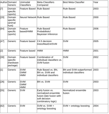
Table 1 Classification overview
Feature Based Rule Based Rule Based 2003
[20] Domain
specific (animal hunt)
Neural Network Rule Based Rule Based 2000
[64] Domain
[47] Generic Feature based C4.5 decision
Chapter 3
Methodology
The initial goal of this thesis was to develop a detector capable of recognizing an abstract high-level concept such as ‘happiness’. This chapter details the basic research that was performed towards that end. This involved choosing a dataset, a supervised learner, and a video annotation tool. The lessons learned from these investigations led to a revision of the initial research goal.
3.1 Basic terminology
The terminology further used is defined as follows. A low-level feature is a piece of audio, video, or text data that has been extracted from a video fragment. Possible examples are color histograms, Mel-ceptstrum coefficients, or a word frequency count. A supervised learner, or classifier, learns to recognize these features and to associate them with a particular semantic concept. A semantic concept is the generic term encapsulating a particular notion or idea. For example, a ‘car’ would be a semantic concept, as it conveys the notion of a particular type of motorized vehicle. In TRECVID terminology, a semantic concept is called a ‘high-level feature’, but that usage is not employed in this paper. Most concepts have a direct link to the feature space. A concept is termed, level, when the concept has a particularly abstract definition. A high-level concept cannot easily be recognized by a classifier operating on the existing feature space, although a human may easily be able to do so. This is known as the semantic gap. Concepts such as ‘love’, ‘happy’, ‘sad’, or ‘anger’ are all examples of high-level concepts. Since high-level concepts are not readily detectable from the feature space, than can only be inferred from other concepts. One might even coin the term, intermediate-level concepts, for the concepts that serve as indicators of a high-level concept. For example, ‘crying’ or ‘funeral’ are intermediate-level concepts indicative of ‘sadness’.
3.2 Choosing a video annotation tool
Given a video source, every defined concept requires an associated ground-truth file. This file lists the frames of the video in which a concept occurs, and is required for the machine learning process. The features in the specified frames are used to train a detector to recognize that particular concept. This means, that at a minimum, ground-truth annotations have to be created for the high-level concept that is the goal of this research. Creating ground-truth annotations is a time intensive task, as one must examine each frame one at a time, marking the presence of the desired concept.
3.3 Choosing a dataset
Choosing a video dataset on which to perform experiments is not a trivial issue, as there are a number of factors influencing the decision process. The more abstract the desired high-level concept, the harder it is to create a detector for it, as less low-level features have a direct bearing on the concept. This means that most of the contribution must come from the detection of intermediate concepts, rather than from feature space. For example, the abstract concept ‘sadness’ might only be inferred from concepts such as ‘crying people’ or ‘funeral’. The immediate consequence of this is that one must also consider whether these intermediate concepts are also present in any dataset. These too then, must have ground-truth annotations created for them. One would need a large digitized video collection to even contain sufficient instances of all the necessary intermediate and high-level concepts, and additionally one would have to make the annotation effort.
This led to consider the TRECVID 2005 corpus, which seemed sufficiently large at 169 hours of news video footage, and had several collections of concept lexicons with associated ground truth annotations. These are: the LSCOM-lite set [35], the MediaMill Challenge set [43], and the complete LSCOM set [32].
LSCOM-lite
The LSCOM-lite set was the result of a common annotation effort by the TRECVID-2005 participants, and contains the ground truth annotations for a collection of 39 concepts. The aim of the LSCOM-lite set was to maximally partition the semantic space, using a minimal amount of concepts, analogous to partitioning the space into a set of hyper cubes. After considering a study of what events were considered newsworthy, the LSCOM-lite developers chose 7 dimensions, each segmented by concepts chosen for their ease of detection and the frequency in which they appeared in search tasks. Most of the concepts from the TRECVID 2003 feature extraction task were included in this set. The annotation software used for this set operated on a static key frame level, thus restricting the concepts to ones that could be identified visually. Temporal concepts, or concepts relying on audio features, could not be used. [35] The deliberate choice for semantically diverse concepts, and the lack of sufficient intermediate level concepts, makes this collection a poor basis for the development of a high-level concept detector.
MediaMill
The MediaMill challenge set augmented the LSCOM-lite lexicon, to arrive at a total of 101 concepts. However, the MediaMill developers maintained the same requirement of visual-only concepts as the LSCOM-lite developers did [35]. Worthy of mention however, is that the MediaMill Challenge set also includes the low-level features with the ground truth annotation of each frame. In addition, optimized detectors are provided for each concept [43].
LSCOM
The LSCOM annotation set, first used for TRECVID 2006, has a larger set of concept annotations, for a total of 856 concepts. However, only half of these actually occur in the TRECVID 2005 video footage. Nonetheless, some of the concepts include in this set are intermediate level concepts, and as such are of greater value towards developing a high-level concept detector. [32]
hierarchy that could ultimately be used to deduce the presence of high-level concept such as ‘happiness’, ‘anger’, and ‘sadness’. However, no low-level features or concept detectors were included, and therefore the choice of dataset fell to the more limited MediaMill challenge set.
3.4 Choosing a Supervised learner
The literature survey from chapter 2 lists a number of classification methods that have been used in research to perform concept recognition. They included knowledge-based schemes, Bayesian classifiers, neural network classifiers, Hidden Markov Models (HMM), and Support Vector Machines (SVM).
Knowledge-based approaches in literature were always restricted to a fixed domain, and were not readily extensible to include new concepts. As a result, I rejected this approach, as it seemed unlikely that any rule-based system would perform robustly when tested against a generic video stream.
Comparative studies from the literature survey of chapter 2 have shown that SVM outperformed the above-mentioned methods in terms of classification performance. The success of SVM performance is due to its sophisticated training procedure, which involves mapping input vectors to a higher dimensional space, thus simplifying the task of finding a maximally separating decision boundary. For more specifics, see Appendix A. Besides superior classification performance, SVMs have also been reported as being capable of handling high-dimensional feature vectors without any detrimental effects, as well as being capable of functioning when given only few training examples. For these reasons the decision was made to use SVMs as the supervised learner of choice for the classification experiments performed in this study.
3.5 SVM in practice
Section 3.3 discusses three lexicons of semantic concepts and their associated ground truth annotations. Although the full LSCOM annotation set formed the best basis for defining high-level semantic concepts as it had the richest concept set, only the MediaMill Challenge set was ready for immediate SVM classification experiments given its inclusion of low-level features for each semantic concept in the set. Thus the MediaMill data set is used for the first experiments with SVM classifiers, as the data set permitted the conduct of early and late fusion classification experiments for comparison against the baseline results.
From a literature survey, it transpires that by far the most predominant SVM classifier in use is LIBSVM [12]. The second most cited SVM classifier is SVM-Lite [28], which is optimized and extended with a graphical user interface called SVM-Dark [37]. Both were installed on a 3.2 Ghz home computer. An initial experiment was conducted using SVM-Dark on the MediaMill experiment 3 ‘beach’ concept, which consists of 120 features. SVM-Dark was tasked with finding the optimum parameters for a new ‘beach’ detector. To perform 10 iterations on a reduced instance of the training set took 3 hours. The full 40 megabyte training set ran for over 15 hours, occupied 4 gigabytes of temporary space, and failed to terminate.
into one class. Both ‘beach’ and ‘dog’ have very few positive training examples, on the order of <50 while there are over 10,000 negative examples.
The lack of positive examples means it is very difficult to train SVM classifiers sufficiently capable of recognizing the ‘beach’ and ‘dog’ concepts. The challenge is in discovering the optimum parameters for the classifiers. (See Appendix A for further information about parameters that influence the creation of a SVM classifier.)
The use of SVM-Dark was discontinued, as LIBSVM was better suited at finding the optimum classifier parameters. On average, parameter learning took between 4 to 10 hours per concept. Eventually successful classifiers for both ‘beach’ and ‘dog’ were created after an exhaustive search for the correct kernel parameters.
3.6 Adjustment of the research approach
The use of any publicly available video source was precluded by the lack of ground truth annotations, and annotating a video source by hand would have proved to be too labor intensive. This led to the examination of three collections of ground truth annotations of the TRECVID 2005 corpus. Of these, the MediaMill dataset was chosen because it was the only collection to contain both the ground truth annotations and the features of each frame, as well as optimized detectors for each concept. Although it would have been possible to create detectors for the concepts in the full LSCOM collection given the MediaMill features, this would have been too computationally intensive. The MediaMill concept lexicon, however, was more limited than the LSCOM collection, and did not have many concepts which semantically indicated a high-level concept. Cursory experiments with the SVM classifier had shown that it was quite hard, and time consuming, to get decent detection results for even some simple concepts within the MediaMill dataset.
Chapter 4
Inter-conceptual boosting experiments
There are various ways to improve the performance of a generic SVM concept detector. Simply selecting better training parameters when generating the SVM model will yield an improvement. Other possibilities are applying different classification schemes such as early or late fusion. The following three experiments aim to improve detector performance by use information about the relationships between concepts. Semantic relationships, as modeled in an ontology, are used by the Ancestor boosting and Sibling-confusion removal techniques. Concept correlations garnered by a Chi-square test, are used by the Chi-square boosting technique. These techniques are used to develop new detectors for each concept in a dataset. These new detectors are compared against the original detectors for each concept, to see whether there is an improvement in the mean average precision (MAP) scores. These scores will be reported and analyzed in order to better understand the effectiveness, and shortcomings, of each technique.
4.1 Experiment Setup
The subsequent experiments were performed on the MediaMill dataset, using the 120 features and detectors from the MediaMill Experiment 3 collection. This particular collection was chosen because it used all possible features (Experiment 1 examines graphical features only, Experiment 2 examines textual features only) and thus the link between features and semantic content in each shot seemed most complete and least indirect (Experiment 4 combines the scores from Experiments 1 and 2, adding a layer of indirection). Early fusion detectors were used as a baseline detector for each concept. Training was performed on a set that consisted of 70% of the data, and results were computed against a test set, consisting of the remaining 30% of the data [43].
The mean average precision (MAP) score is used to compare various concept detector results. This value is computed by taking the average of the precision scores of the relevant shots from a ranked list of detector confidence scores.
Let Precision(i) be the precision at rank i, where precision is defined as the number of relevant and found shots over the set of found shots. Let Relevant(i) be a function which states whether the shot at i is relevant. Then for a concept with N shots of which #relevant are relevant, the MAP score is defined as:
MAP: 1/#relevant * i=1∑N (Precision(i)*Relevant(i))
Mean average precision is a useful metric as it combines precision and recall into one single value. MAP emphasizes returning more relevant shots earlier, and as such is an appropriate choice of metric for comparing concept detectors.
the presence of a highly correlated concept can be used to distinguish ambiguous low-level features.
The first step is to generate the ontology itself, as in the adjacent figure. This was done by calculating the posterior probabilities of each concept against the others in order to determine which concepts were supersets of the others. Given a posterior probability P(A|B), concept A was placed as an ancestor node in the ontology and B as a child node of A when the posterior probability exceeded a certain threshold value. For this experiment, the threshold was set at 95%. This results in a natural hierarchy that reflects the relationships of the concepts within the data set. The focus of the following experiment was to enhance concept classifiers which shared the same sibling axis. Examples of this are the concepts {government, building, house, and tower}, which have the ‘building’ parent concept. The concepts are related semantically on the parent axis, but are semantically mutually exclusive on the sibling axis. Since only posterior probabilities were used to generate the ontology, this procedure is inadequate to definitely conclude that sibling classes are mutually exclusive.
4.2 Experiment 1: Sibling-confusion
removal
Sibling concepts are semantically very related, and this tends to be reflected in their feature sets, which also are likely to be very similar. This causes confusion among their concept detectors, which are unable to distinguish the features correctly, resulting in many false positives. Based on work by Wu [48], the Sibling-confusion removal technique reduces the amount of false positives detected by normalizing detector scores based on the confusion factor, a number that indicates the likelihood of a false positive occurring for a particular shot.
Intuitively, the confusion factor is only an important consideration when a shot scores highly on two or more sibling class detectors. Only one detector can be correct, and the others must be detecting false positives (because mutual exclusivity is assumed on sibling classes in the ontology, due to their semantic meanings). Formally, given shot s, concept Ci, and the set of
concepts Csibling, which are the sibling concepts of Ci, the confusion factor is defined as
P(s|Ci)-max(P(s|Csibling)), the difference between the probability that s is an example of Ci and the
highest scoring sibling concept. P(s|Ci) is the confidence score given by the SVM classifier for
that concept. For this experiment, an early fusion (MediaMill experiment 3) type classifier was used, that learned each concept from 101 low-level features.
The initial confidence score P(s|Ci) for each concept in the data set must be updated to take
the confusion factor into account. As such, the general equation for this update becomes:
P(s|Ci)updated= P(s|Ci)initial* f(confusion factor),
where the confidence score is updated as a function of the confusion factor:
P(s|Ci)updated = P(s|Ci)initial * |f(P(s|Ci)initial -max(P(s|Csibling))|
The function max simply returns the highest scoring sibling concept, P(s|Csibling)), of Ci.
Several considerations, such as the magnitude and sign of the confusion factor, have to be taken into account when determining the function. A small confusion factor implies that there are two highly scoring concept detectors (or trivially two low scoring ones). This in turn means that P(s|Ci)updated ought to be significantly smaller, as to reflect the uncertainty of placing shot s in the
correct concept class. A large, positive confusion factor on the other hand, implies that shot s is most likely of class Ci and not likely to occur in any of the sibling classes. As such, P(s|Ci)updated
must remain large. The large, negative confusion factor case implies that shot s is most likely a member of Csibling and unlikely to be a member of Ci. As such, it is safe to reduce the score of
P(s|Ci)updated even more. Finally, one must consider the rate of change between each of the
extremes presented above. A large positive confusion factor requires that P(s|Ci)updated stay large,
while a small confusion factor requires a sharp drop in P(s|Ci)updated. This suggests that the
relationship between confusion factor and P(s|Ci)updated is non-linear, and in fact ought to be exponential. The function f(x)=ex meets all these requirements resulting in:
P(s|Ci)updated = P(s|Ci)initial * e (P(s|Ci)initial -max(P(s|Csibling))
The final step is to normalize the results back into the range [0-1]
P(s|Ci)updated = P(s|Ci)initial * e (P(s|Ci)initial -max(P(s|Csibling)) /e
In essence, this formula can be thought of the normalization of confidence scores based on the interference from closely related sibling classes. This formula was used to update the confidence scores of the sibling concept detectors in the MediaMill dataset, for which afterwards the MAP was computed. The results obtained by executing Sibling-confusion removal on the test set are presented in Annex 2, with an analysis thereof in the following section, 4.3.
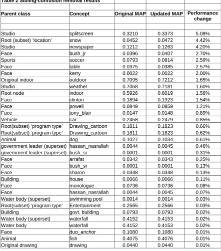
4.3 Sibling-confusion removal analysis
0.60, and the concept ‘outdoor’, from 0.71 to 0.72, should be taken as a qualified success however. What then, however, are the reasons for the general decrease in MAP over many sibling-concept groupings?
At the start of the experiment, it was hypothesized that all sibling groupings had to be mutually exclusive. More correctly, such a set has to be closed, and each concept within has to be complementary to all the others. That is to say, assuming parent concept Cp was detected in
shot s, one, and only one, of the child concepts that made up the sibling concept set also had to be detected in the shot,
∀Ci∈Cp• Ci occurs in s→∀Csibling∈Cp• Csibling≠ Ci→ Csibling does not occur in s.
Although these properties fortuitously hold for the set {indoor, outdoor}, this however could not always be enforced for other groupings.
In part, the fault lies with the automated ontology determination process. Although it was able to determine parent-child relationships, it was not able to adequately group the various sibling concepts according to their semantic relationships. As a result, ‘tony blair’ was omitted from the government leader set of {allawi, arrafat, bush_jr, bush_sr, hu_jintao, kerry, lahoud, powell}, thus violating the desired closure property. Likewise an unrelated group of siblings such as {anchor, duo_anchor, newspaper, splitscreen, weather} was entirely possible too, thus violating the property that each element had to be the complement of the remainder of the set. The failure to make the correct sibling sets at the semantic level means that the confusion removal algorithm is doomed to failure prior to execution.
The following example illustrates the effects of violating the closure rule when creating set groupings. In this scenario, the sibling concepts are Ci, Cj, and Cmissing. Cmissing is so termed because
it is alternately included in the set of sibling concepts in the ontology.
Consider again the formula: P(s|Ci)updated= P(s|Ci)initial * e (P(s|Ci)initial -max(P(s|Csibling)) /e.
Let shot s contain the concept Cmissing, and let the initial detector scores be {P(s|Ci)=0.40,
P(s|Cj)=0.41, P(s|Cmissing)=0.9}initial.
The first case is when Cmissing is included in the sibling concept set. Because Ci and Cj are
semantically related to Cmissing, they get an ambivalent detector score on shot s. However, because
shot s scores so highly on concept Cmissing, there is a sharp drop in their modified predictions after
confusion removal, {P(s|Ci)=0.089, P(s|Cj)=0.092, P(s|Cmissing)=0.54}.
The second case is when Cmissing is omitted from the sibling concept set, the scores then after
confusion removal are: {P(s|Ci)=0.145, P(s|Cj)=0.152}, which is less of a decrease in confidence
estimations. This in turn impacts the mean average precision score, as it computes, per concept, the average precision over a list sorted according to confidence scores. Thus P(s|Ci)=0.089
(Cmissing not omitted) would correctly rank lower on the list than P(s|Ci)=0.145 (Cmissing omitted).
The other case to be considered is when the elements in a set are not all complementary to the rest, per the requirement: ∀Ci ∈Cp • Ci occurs in s→∀Csibling ∈Cp • Csibling ≠ Ci → Csibling
does not occur in s. Consider three concepts, {Ck, Cl, and Cm}. Concepts Ck and Cm are sibling
concepts, while Cl is an independent concept, unrelated to both. Let shot s contain the concepts Ck
and Cl, and let the resultant detector scores be {P(s|Ck)=0.93, P(s|Cl)=0.92, P(s|Cm)=0.11} initial.
Ck and Cm are complementary over shot s, which is reflected in their confidence scores, and
approximate 1 and 0 respectively. Cl is independent of either however. Because it is present in the
sibling group its confidence score is included in the calculation, which entirely ruins the updated scores and the resultant MAP score, {P(s|Ck)=0.34, P(s|Cl)=0.33, P(s|Cm)=0.02} (incorrect- Cl is
(correct- Cl is excluded). In a rank ordered list, the incorrect scores, from the inclusion Cl in the
calculations, would be much lower on the list, relatively, and would thus lower the MAP score.
Thus the presence of an extraneous concept or the absence of one as a result of a poorly constructed ontology can lower the MAP scores of all the concepts in the resultant sibling sets. This undoubtedly played a significant role for the generally lower scores, but is not the entire explanation, as even groupings which have been amended to ensure the set properties discussed above perform worse after confusion removal. Examples of this are the sets {male, female} or {drawing, cartoon}
There is a simple, numeric explanation that also must be considered. Confusion removal is a normalization operation, due to the division of the re-ranked score by e.
Recall:
P(s|Ci)updated= P(s|Ci)initial * e (P(s|Ci)initial -max(P(s|C sibling))/e.
Inherently, re-ranked scores are lower than their initial values, due to the exponential, e[0-1]<e. The insight however, is that shots which have a lot of confusion, have an exponentially lower value, so in a rank-ordered list, the only positions which change are those of shots with a lot of confusion amongst related concepts. In theory, this should mean that the mean average precision scores for all concerned concepts should stay static, or improve as a result of the lower positions in the ranked list of the false positives. How come then, that the {male, female} set has decreased MAP scores overall? ‘Male’ has an initial MAP of 0.0678, which drops to 0.0675, and ‘female’ has an initial MAP of 0.0609, which drops to 0.0405. The simple answer is that sometimes the detectors themselves are not up to the task. In this example, both the male and female detectors gave low confidence estimates, which tended to 0. Shots which contained the concept and shots that did not, received indistinguishable estimates. The lack of detector certainty is compounded in the exponent, which approached 0, resulting in a larger drop in the ranked list.
The final consideration is that the confusion removal algorithm only works if there are, in fact, false positives to remove. If there are none, the algorithm only causes a decrease in the MAPs of the concepts under consideration. An example of this occurrence is the animal
grouping, consisting of {bird, dog, fish, horse}. All set properties discussed previously are valid for this grouping. Nonetheless, the MAP of the bird concept drops from 0.761 to 0.744, the MAP of dog stays at 0.103, the MAP of fish stays at 0.407, as does the MAP of horse at 0.0003. The ideal case would be detectors that gave confidence scores: P(s|Ci)=1 and P(s|Csibling) =0. In
practice however, P(s|Ci)<1 and P(s|Csibling)>0 resulting in a non-trivial value in the exponent, e (P(s|Ci)initial -max(P(s|Csibling))
/e, which causes a change in the position in the ranked list of a shot-score, and ultimately a decrease in the concept MAP.
The last point is not too much of an issue, because Sibling-confusion removal runs in linear time with respect to the size of the dataset, and executes quickly. As such, a trial-and-error approach is sufficient to determine the concepts that benefit from the application of this technique.
4.4 Experiment 2: Ancestor boosting
This experiment builds upon the concept ontology from the previous experiment. Instead of considering sibling concepts it focuses on the parent-child relationship between concepts. That is, the concern here is the concepts which are semantically related, where a parent concept is the superset of the child concept. For example, the concept ‘water body’ encompasses the concepts beach, river, swimming pool, and waterfall in their entirety. The goal is to improve the performance of a child-concept detector by considering the results from the related parent-concept detector. This is a more detailed examination of a technique first done by Wu [48].
Fewer concept examples are present in the dataset in general when a concept is semantically more specific. This adversely impacts the training phase of such a concept detector, and results in a less robust detector. Ancestor concepts, however, have broader semantic definitions and thus occur more frequently in the data set, and as such are detected more robustly. The idea behind this experiment is to leverage the performance of the more accurate and powerful ancestor-concept detectors to boost the performance of their child-concept detectors. Since the ancestor and child concepts are semantically related it seems plausible to combine the results of their detectors. Thus one compensates for a less accurate, but specifically targeted, child concept detector by using a more robust ancestor detector with a broader semantic coverage.
Thus a child concept detector is a linear interpolation of all the ancestor detectors, whose weights are determined in a training phase. The figure below illustrates the idea.
Expressed formally, the updated confidence detector for child concept Ci, given shot s
and ancestor concepts {Cj … Ck}, would have the following formula:
P(s|Ci)’= λiP(s|Ci)+ λjP(s|Cj)+…+ λkP(s|Ck)
The parameters λare determined by empirically finding the optimum weights through the use of the Expectation Maximization (EM) algorithm detailed in [34] and presented below:
1. A concept grouping is selected, consisting of a child concept {C1}, and its ancestors,
2. Each λ1…λn is initialized with a random number in the range [0-1].
Steps 3 and 4 are iterated until λi converges:
3. For every concept Ci ∈{C1,C2…Cn}
For every shot s in the set of shots predicting the child concept, C1
βi = ∑s∈S(λiP(s|Ci)/ ∑mλj mP(s|Cj)m)
4. λi=βi /∑βj
After sufficient iterations, λi will have been determined. These can then be used to update the
shot scores for that particular child concept detector.
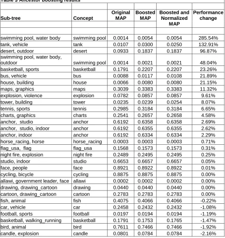
New child concept detectors were created for all child concepts in the MediaMill dataset by interpolating various ancestor-child concept combinations. The λ parameters were determined for all concepts in a particular ancestor-child set, by running the EM algorithm detailed above against the training set. In this experiment, 30 iterations were done. MAP scores for each concept were determined after performing Ancestor boosting on them, using the recently discovered λ
parameters on each ancestor-child concept in the test set. The results are presented in Annex 3 and analyzed in 4.5. The original MAP scores for child concepts are listed, followed by the MAP scores after ancestor boosting. Some concepts in the training set did not have scores in the full range [0-1], and were first normalized for compliance before the EM algorithm was applied. This affected the λ values, and changed the resultant MAP scores, which is also displayed. For comparison purposes, sometimes an ancestor concept was omitted from a sub tree.
4.5 Ancestor boosting analysis
In this experiment, 17 out of 61 distinct concepts had improved MAP scores. The assumption behind this experiment was that child concepts only occur rarely in a dataset, and thus have weak concept detectors. These child detectors are insufficiently able to recognize the low-level features that determine the semantic meaning of the concept. Ancestor concepts, on the other hand, occur more often, and thus have stronger detectors. Since semantically a child concept is automatically a subset of the parent concept, the assumption is that the low-level features that determine the child concept are also the features that determine the parent concept. Thus it should be possible to interpolate the scores from the ancestor and child concept detectors for a particular shot, and arrive at a more definitive detector than the original. This should be conceived of as the expansion of the classification boundary of the child detector, based on the classification boundaries of the ancestor concepts. This section analyzes and reflects upon the results garnered from the application of the ancestor boosting method on the MediaMill dataset.
Of the 94 sub-trees, 18 concepts had better MAP scores when normalization occurred before boosting, 11 had worse scores, and the remainder were unaffected by normalization. Since the MAP results with normalization were generally slightly better, these values are cited in subsequent passages. Out of 94 sub-trees, 21 gave improved results after ancestor boosting, while the remainder performed worse. The most noticeable improvements were the sub-trees {desert, outdoor}, where the ‘desert’ MAP improved from 0.093 to 0.183 (96% increase), {anchor, studio, indoor}, where the ‘anchor’ MAP improved from 0.619 to 0.635 (2.6% increase), and {swimming pool, water body}, where the ‘swimming pool’ MAP improved from 0.0014 to 0.0054 (285% increase). The remaining 73 sub trees, whose detectors performed worse after boosting, had MAP scores that sometimes varied mildly, but sometimes by as much as one significant figure.
There are two possible causes for the variations in MAP amongst the sub-trees:
The semantic distance between concepts; and
The semantic distance is the subjective measure of the closeness in meaning of two concepts. In the context of the ontology of the dataset, ‘building’ is semantically close to ‘house’, while ‘building’ is rather more semantically distant from ‘outdoor’. Although these concepts share the same ancestor-descendant axis,